Unsupervised Adaptation of Deep Speech Activity Detection Models to Unseen Domains

Abstract

Speech Activity Detection (SAD) aims to accurately classify audio fragments containing human speech. Current state-of-the-art systems for the SAD task are mainly based on deep learning solutions. These applications usually show a significant drop in performance when test data are different from training data due to the domain shift observed. Furthermore, machine learning algorithms require large amounts of labelled data, which may be hard to obtain in real applications. Considering both ideas, in this paper we evaluate three unsupervised domain adaptation techniques applied to the SAD task. A baseline system is trained on a combination of data from different domains and then adapted to a new unseen domain, namely, data from Apollo space missions coming from the Fearless Steps Challenge. Experimental results demonstrate that domain adaptation techniques seeking to minimise the statistical distribution shift provide the most promising results. In particular, Deep CORAL method reports a 13% relative improvement in the original evaluation metric when compared to the unadapted baseline model. Further experiments show that the cascaded application of Deep CORAL and pseudo-labelling techniques can improve even more the results, yielding a significant 24% relative improvement in the evaluation metric when compared to the baseline system.

1. Introduction

Speech Activity Detection (SAD) aims to determine whether an audio signal contains speech or not, and its exact location in the signal. This constitutes an essential preprocessing step in several speech-related applications such as speech and speaker recognition, as well as speech enhancement. In many cases, SAD is used as a preliminary block to separate the segments of the signal that contain speech from those that are only noise. This way, enabling the overall system to process only the speech segments. A large number of approaches have been proposed for the SAD task. Traditionally, statistical approaches have been used with relevant results under the assumption of quasi-stationary noise. Several works rely on the extraction of specific acoustic features [1,2]. Conversely, other methods are model-based [3,4], aiming to estimate a statistical model for the noisy signal. Additionally, some unsupervised approaches can also be cited: based on energy [5], or based on the estimation of the signal long-term spectral divergence [6]. Recently, deep learning approaches are becoming increasingly relevant in the SAD task. The research presented in [7] implements a SAD system based on a multilayer perceptron with energy efficiency as the main concern. A deep neural network (DNN) approach is used in [8] to perform SAD in a multi-room environment. In [9], new optimisation techniques based on the area under the ROC curve are explored in the framework of a deep learning SAD system.

Recurrent neural networks (RNN) are significantly useful when dealing with temporal sequences of information because they are able to model temporal dependencies introducing a feedback loop between the input and output of the neural network. Several applications of long short-term memory (LSTM) networks [10] can be cited in the SAD task [11,12]. Some of our latest solutions for SAD in the context of diarisation applications obtained competitive results applying a bidirectional LSTM-based classifier [13,14]. Convolutional Recurrent Neural Networks (CRNN) combine the capability of convolutional networks to capture frequency and time dependencies simultaneously seeking to extract discriminative features, and the capability of recurrent networks to deal with temporal series. A number of examples of the use of CRNN models in audio processing can be found in the literature [15,16]. CRNN models have been also applied to the SAD task with relevant results [17].

In the last few years, a number of international evaluation campaigns have been proposing the SAD task as one of their challenges, seeking to advance this kind of systems in a variety of challenging domains. In this context, the National Institute of Standards and Technology (NIST) introduced the OpenSAT evaluations starting in 2017 [18]. Three domains were proposed for the SAD task: public safety communications, low resource languages and audio extracted from YouTube videos. Post-evaluations analysis revealed a significant difference in performance among the three domains for most participant teams. Similarly, aiming to motivate the research effort on a demanding domain such as audio from Apollo space missions, a series of annual challenges has been held since 2019 [19] proposing the SAD task among other speech related tasks. This initiative has resulted in the digitisation of the original analogue recordings from the space missions. Part of this data has been made available through the Fearless steps (FS) corpus, consisting of a cumulative 19,000 h of conversational speech coming from the Apollo 11 mission [20]. Audio data belong to 30 different communication channels, with multiple speakers in diverse locations. Most channels show a strong degradation with transmission noise or noise due to tape ageing.

Whereas current SAD state-of-the-art solutions rely on the use of deep learning techniques, these applications depend strongly on the amount of labelled data available. In some specific scenarios, obtaining labelled data can be significantly expensive or even impossible, which is why unsupervised domain adaptation techniques are an active research topic [21,22]. Domain adaptation techniques aim to transfer the knowledge obtained from a source domain and transfer it to a target domain. In addition, unsupervised domain adaptation techniques work under the constraint that no labels are available in this new target domain. Inspired by our previous experiences participating in the Fearless Steps Challenge [23,24], that introduced a new audio domain in the research community, in this paper we aim to explore unsupervised domain adaptation techniques in the context of the SAD task. Considering a SAD model trained on different well-known domains in the SAD task, such as broadcast or meetings, with huge amounts of labelled data available, we evaluate three possible ways to adapt the SAD model to a new unseen domain in an unsupervised way. Results are presented using the data provided in the Fearless Steps Challenge; however, the techniques and methods described in this paper are described in a general way so that domain adaptation could be done on any possible scenario. Unlike the work presented in [25], where the key idea is to perform a pretraining process on DNN models using unlabelled data, seeking to obtain a shared representation, this work aims to perform unsupervised domain adaptation directly on the model space, with the objective of fine tuning a given model trained previously with labelled out of domain data.

The remainder of the paper is organised as follows. Section 2 introduces the domain adaptation problem, presents some approximations found in the literature on how to solve it, and introduces different methods evaluated. Section 3 presents the experimental setup, describing the neural network architecture, datasets considered and metrics used in the evaluation. In Section 4, results for the baseline SAD system and unsupervised adaptation techniques are described. Finally, a summary of the work and conclusions are presented in Section 5.

2. Domain Adaptation

Usually machine learning algorithms require large amounts of manually labelled training examples in order to train a reliable model. In real applications, however, obtaining labelled data requires huge efforts and, in some cases, it is even impossible. A simple and straightforward solution is to train a model on a labelled dataset which is somehow related to the target data and then apply it to the data being considered. This approach is likely to lead to substantial drops in performance caused by the domain shift, observed in the different feature and label distributions [26]. In order to solve this problem, several domain adaptation techniques have arisen, aiming to learn from a source dataset and transfer that knowledge obtained to a target dataset. Domain adaptation is currently an active research topic in the machine learning community [27,28]. Focusing on speech technologies applications, several works have also investigated the domain adaptation problem for speech recognition [29], speaker recognition [30] or speech enhancement [31].

2.1. Problem Formulation

In the following lines, a formal introduction to the domain adaptation problem and some definitions relevant to the topic are provided. In order to formulate the domain adaptation problem, two domains need to be defined: the source and the target domain. The source domain, $D_s$, represented by a source dataset ${\mathsf{\Pi }}_s=\{{\mathbf{X}}_s,{\mathbf{Y}}_s\}$ where ${\mathbf{X}}_s=\{x_{s_1},\dots ,x_{s_N}\}$ is the set of acoustic features with N examples, and ${\mathbf{Y}}_s=\{y_{s_1},\dots ,y_{s_N}\}$ the speech labels defining each of the elements in ${\mathbf{X}}_s$ as speech or non-speech examples. Similarly, the target domain, $D_t$, is represented by a target dataset ${\mathsf{\Pi }}_t=\left\{{\mathbf{X}}_t\right\}$ where ${\mathbf{X}}_t=\{x_{t_1},\dots ,x_{t_M}\}$ is the set of acoustic features with M examples. In the case of unsupervised domain adaptation problems, such as the ones described in this work, no ground-truth labels ${\mathbf{Y}}_t$ are available for the target dataset.

Traditionally, in supervised learning problems training samples are assumed to be available. This is the case for the source domain. Accordingly, the learning problem is to determine a classifier $f_s({\mathsf{\Pi }}_s,{\theta }_s)$ that allows obtaining high classification accuracy for test samples by exploiting the available training set ${\mathsf{\Pi }}_s$. The classifier is described by a set of parameters ${\theta }_s$ specific for each family of classifiers.

In the domain adaptation framework, the problem becomes more complex as test samples are drawn for a target domain distribution different from the source domain distribution of training samples. Considering the ideas described, the goal of domain adaptation techniques should be to develop a new classifier $f_t({\mathsf{\Pi }}_s,{\theta }_s,{\mathsf{\Pi }}_t,{\theta }_t)$ that obtains an accurate prediction of test samples coming from the target domain by exploiting labelled training samples ${\mathsf{\Pi }}_s$ from the source domain $D_s$ and unlabelled samples ${\mathsf{\Pi }}_t$ from the target domain $D_t$. As for supervised classifiers, this new model adopted for classification is described by a set of parameters ${\theta }_s$ specific for each family of classifiers, and by a set of parameters ${\theta }_t$ which is specific to each domain adaptation technique.

2.2. Approaches to Domain Adaptation

In order to better understand the domain adaptation problem, a variety of works over the years have tried to categorise the diverse conditions found for the problem. We refer the reader to the following survey for a more detailed description of this categorisation [32]. The first level of categorisation refers to the relation between source and target domains. Under the assumption that the source and target domain are directly related, transferring knowledge can be performed in a single step. This is usually called one-step domain adaptation. In case that assumption fails, one-step domain adaptation may not be effective. Multi-step domain adaptation [33] aims to connect two unrelated domains via a series of intermediate bridges, and then perform one-step domain adaptation.

In this work, as human speech has characteristics that may not vary among domains, we assume that source and target domains are related. Because of that, we focus on one-step domain adaptation solutions. In this scenario, domain adaptation approaches can be summarised intro three big cases according to the work in [34]:

• Discrepancy-based: this family of solutions works under the assumption that fine-tuning a model using labelled or unlabelled data can reduce the shift between source and target domain. Under this idea, several criteria can be used to perform domain adaptation: some authors use class information to transfer knowledge between two domains [35]. The authors of [36,37] seek to align the statistical distribution shift between source and target domain. Other approaches also aim to improve generalisation by adjusting the architectures of DNNs, such as the work presented in [38].
• Adversarial-based: in this case, a domain discriminator tries to identify whether a data point belongs to the source or the target domain. This is used to encourage domain confusion through an adversarial objective that minimises the distance between source and target domain distributions. Two main groups can be observed when implementing this idea: those relying on generative models such as generative adversarial networks (GAN) [39], or those that rely on non-generative models that aim to obtain domain invariant representation through a domain confusion loss [40].
• Reconstruction-based: This approach is based on the idea that data reconstruction of the source or target samples may be helpful in order to improve the domain adaptation process. This way the reconstructor is able to ensure both specificity of intra-domain representations and indistinguishability of inter-domain representations. Some examples of these methods can be cited, such as the use of an encoder-decoder reconstruction process [41], or an adversarial reconstruction obtained via a cycle GAN model [42].

2.3. Unsupervised Domain Adaptation Techniques

Following the categorisation previously explained, in this paper we focus our efforts on the evaluation of one-step, discrepancy-based domain adaptation techniques. Additionally, the three methods presented are fully unsupervised, meaning that no labels for the target domain are needed in order to obtain an adapted model. Descriptions of these methods are presented in the next subsections.

2.3.1. Pseudo-Labelling

The goal of pseudo-labelling (PL) [43] is to generate a set of predicted labels for unlabelled samples with a model trained on labelled data. This idea is an intuitive and straightforward application that can help overcome the challenge of collecting large labelled datasets. Several works in the literature have explored different algorithms for creating pseudo-labels. In [44], pseudo-labels are assigned to unlabelled samples using neighbourhood graphs. The idea of pseudo-labelling is extended in [45] by incorporating confidence scores for unlabelled samples. The authors of [46] present a new optimisation framework to iteratively update the obtained pseudo-labels. Our approach is inspired by the works in [43,47], where pseudo-labels are generated directly as the predictions of a trained neural network.

Our solution for pseudo-labelling domain adaptation can be described according to the three following steps:

• Train source model: first, an initial model is trained in a supervised way on the source domain.
• Predict target labels: the initial model is then used to predict speech presence or absence for the unlabelled target domain.
• Adapt using predicted labels: finally, the initial model is retrained in a supervised way using the pseudo-labels as if they were true labels.

Furthermore, besides performing a fine tuning of the initial source model to obtain the target model, this solution could also be used to train a target model from scratch using the obtained pseudo-labels or a combination of the source labelled data and the obtained pseudo-labels. Pseudo-labelling techniques have been used in several audio processing applications ranging from acoustic classification problems [48], diarisation [49] or speech recognition [50] with relevant results. In this work, we aim to extend the pseudo-labelling techniques to the SAD task and evaluate its performance in the framework of domain adaptation.

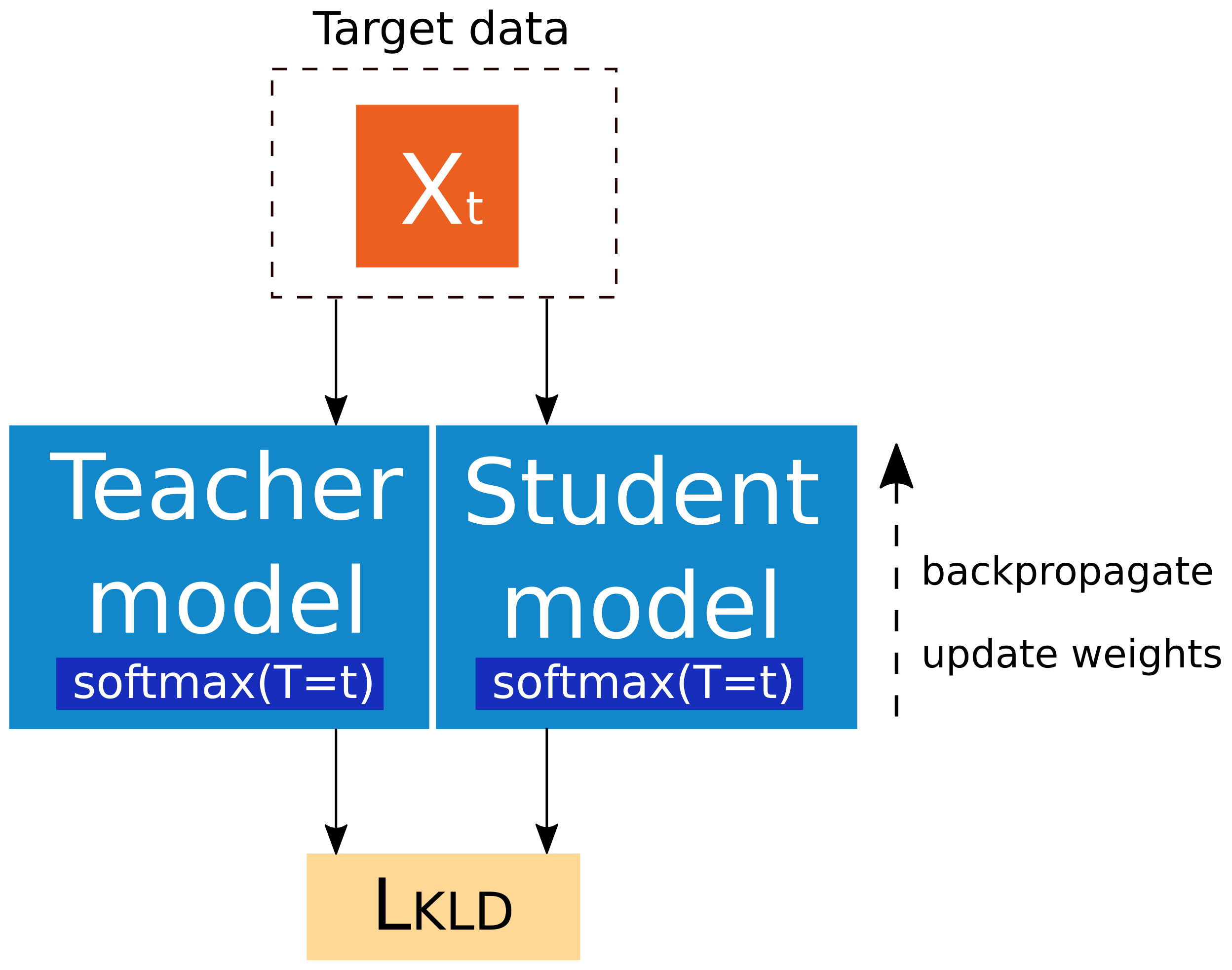
2.3.2. Knowledge Distillation

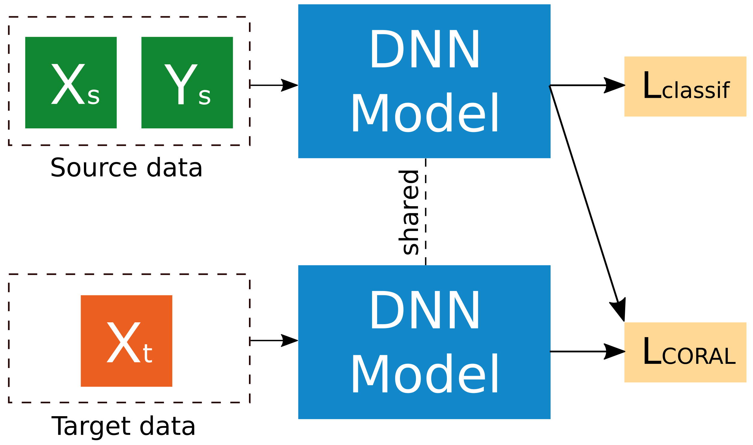
The knowledge distillation (KD) [51] framework was originally proposed as a model compression method in which two DNNs are involved. These two models are usually known as teacher and student model in an analogy to the education process. The main idea of this philosophy is that the teacher model produces soft labels which are used to train the student model. Consequently, the student model should imitate the predictions of the teacher model. In order to do so, Kullback–Leibler Divergence (KLD) loss between student and teacher distributions is minimised. KLD loss can formulated according to the following expression:

$$\mathrm{KLD}=-\sum _{i=1}^I{p}_t\left(y_i\right|x_i)log\left(\frac{p_s\left(y_i\right|x_i)}{p_t\left(y_i\right|x_i)}\right),$$

(1)

where i is the example index, $x_i$ is the input example, $p_t\left(y_i\right|x_i)$ is the output posterior probability of the label $y_i$ from teacher model and $p_s\left(y_i\right|x_i)$ is the output posterior probability of the label $y_i$ from student model for the same example. As done in most KD methods [52,53], the teacher model is usually frozen, relying on a pretrained model, in order to reduce complexity. In this case, where only the parameters of the student network need to be optimised, minimising KLD loss expressed in Equation (1) is equivalent to minimising the expression shown in the following equation:

$$L_{\mathrm{KLD}}=-\sum _{i=1}^I{p}_t\left(y_i\right|x_i)log\left(p_s\left(y_i\right|x_i)\right)+const,$$

(2)

where $const$ is a constant term as defined in [54]. As it has just been explained, knowledge is transferred via the minimisation of a loss function whose target is the distribution of class probabilities predicted by the teacher model. This is the output of a softmax function applied on the teacher model logits. However, in most cases, this distribution provides a high probability for the correct class, with the other class probabilities close to zero. In order to address this issue, the authors of [51] introduced the concept of softmax temperature. The probability $p_i$ of the class i is calculated from the neural network logits z according to the following equation:

$$p_i=\frac{e^{\left(\frac{z_i}{T}\right)}}{{\sum }_i{e}^{\left(\frac{z_i}{T}\right)}},$$

(3)

where T is the temperature parameter. For the case of $T=1$ the standard softmax function is obtained. As T grows, the probability distribution generated becomes softer, providing more information as to which classes the teacher found more similar to the predicted class.

The proposed experimental setup for KD based domain adaptation is shown schematically in Figure 1. It can be seen that both models—teacher and student—receive target data examples ${\mathbf{X}}_t$ as input. Predictions from both models are obtained via softmax activations using the same temperature parameter t. Soft predictions from the teacher network are used to transfer knowledge to the student network, aiming at mirroring those predictions using the mentioned KLD loss. In this process, the teacher model is frozen and only parameters of the student model are updated. In order to test the system, the teacher model is discarded, and final predictions are obtained using the student model with a standard softmax activation with $T=1$. As it is implemented, this version of KD can be interpreted as a soft version of the pseudo-labelling method previously described.

Several examples of the use of KD techniques for solving the domain adaptation task can be found in the literature. The authors of [55] apply KD to improve acoustic models for automatic speech recognition (ASR) in application-specific conditions. Something similar is done in [56], that uses KD algorithms to improve ASR performance in noisy environments. Concerning the SAD task, we can also see several examples of the teacher student architecture being used in domain adaptation solutions [57,58].

2.3.3. Deep CORAL

The recently proposed Correlation Alignment (CORAL) method [37] is an unsupervised adaptation technique that is performed by aligning the second-order statistics of the source and the target distributions. However, this technique relies on a linear transformation and is not end-to-end. In order to address those issues, an extension on the CORAL method named Deep CORAL was proposed [59] with the idea of incorporating the CORAL technique directly into deep neural networks by constructing a differentiable loss functions that minimises the difference between source and target correlations.

The CORAL loss between two domains for a single feature layer is described in the following lines. Suppose a set of training examples coming from the labelled source domain, $D_s$, described by ${\mathbf{U}}_s=\{u_{s_1},\dots ,u_{s_N}\}$ with $u\in {\mathbb{R}}^d$, and unlabelled target data ${\mathbf{V}}_t=\{v_{t_1},\dots ,v_{t_M}\}$, with $v\in {\mathbb{R}}^d$. The number of source and target data are N and M respectively. As described in the original paper, ${\mathbf{U}}_s$ and ${\mathbf{V}}_t$ represent the d-dimensional deep layer activations of a deep neural network model. Considering the provided definitions, the covariance matrices of the source and target data are given by the following equations:

$${\mathbf{C}}_{\mathbf{s}}=\frac{1}{N-1}({\mathbf{U}}_s^T{\mathbf{U}}_s-\frac{1}{N}{\left({\mathbf{1}}^T{\mathbf{U}}_s\right)}^T\left({\mathbf{1}}^T{\mathbf{U}}_s\right)),$$

(4)

$${\mathbf{C}}_{\mathbf{t}}=\frac{1}{M-1}({\mathbf{V}}_t^T{\mathbf{V}}_t-\frac{1}{M}{\left({\mathbf{1}}^T{\mathbf{V}}_t\right)}^T\left({\mathbf{1}}^T{\mathbf{V}}_t\right)),$$

(5)

where $\mathbf{1}$ is a column vector with all elements equal to 1. The CORAL loss is then defined as the distance between the second-order statistics of the source and target features. This is shown in Equation (6):

$$L_{\mathrm{CORAL}}=\frac{1}{4d^2}{\parallel {\mathbf{C}}_{\mathbf{s}}-{\mathbf{C}}_{\mathbf{t}}\parallel }_{{}_F}^2,$$

(6)

where ${\parallel ·\parallel }_{{}_F}^2$ denotes the squared matrix Frobenius norm.

The idea behind Deep CORAL adaptation technique is to obtain a set of deep features that are both discriminative enough to train a strong classifier and invariant to the change observed between source and target domains. Minimising a classification loss by itself, as usually done in supervised learning approaches, may lead to overfitting on the source domain and a reduced performance on the target domain. By contrast, minimising the CORAL loss alone may lead to degenerated features. In order to match the conditions stated above, the final loss to be optimised is a combination of both a classification loss and the CORAL loss. The representation of the neural architecture needed to implement Deep CORAL adaptation technique is shown in Figure 2.

As shown, source features are forwarded through the DNN model and then a classification loss is computed using source labels. Similarly, target features are used in combination with source features to compute CORAL loss. Network parameters are shared among the two DNN models. Considering the described architecture, the joint optimisation target of classification loss and CORAL loss is described in Equation (7):

$$L=L_{\mathrm{classif}}+\sum _{i=1}^z{\lambda }_i{L}_{{\mathrm{CORAL}}_i},$$

(7)

where $L_{\mathrm{classif}}$ is any traditional classification loss function such as cross entropy, z is the number of CORAL loss layers in a deep network and ${\lambda }_i$ is a weight that trades off adaptation and classification accuracy on the source domain. The sum term depicted aims to represent the possibility of incorporating the CORAL loss on additional layers of the DNN architecture. However, as described in the original paper, authors apply the CORAL loss only to the last classification layer in the DNN architecture. In our experiments, we apply CORAL loss in the same way, simplifying Equation (7) to become Equation (8) in the case where $z=1$:

$$L=L_{\mathrm{classif}}+\lambda L_{\mathrm{CORAL}}.$$

(8)

More recently, further work has proposed a new approach built upon the Deep CORAL method. The authors of [60] argue that the Euclidean distance used in the original Deep CORAL proposal may not be the most appropriate way to measure the distance between the source and target domains. Knowing that covariance matrices are positive semi-definite, they can be seen as two points lying on a Riemman manifold, and the metrics defined therein should consider its non-Euclidean structure [61]. Therefore, the Euclidean distance as defined in Equation (6) may be seen as only suboptimal in such a space. Considering this information, the log-Euclidean distance is instead a Riemannian metric that better captures the manifold structure. This metric is defined according to the following equation:

$$d_{log}(\mathbf{X},\mathbf{Y})={\parallel log\left(\mathbf{X}\right)-log\left(\mathbf{Y}\right)\parallel }_{{}_F},$$

(9)

where $log\left(\mathbf{X}\right)$ is the matrix logarithm of $\mathbf{X}$ [62]. Similarly as the CORAL loss, the log CORAL loss can be obtained by replacing the Euclidean distance in Equation (6) with the log-Euclidean distance. This is shown in Equation (10).

$$L_{log\mathrm{CORAL}}=\frac{1}{4d^2}{\parallel log\left({\mathbf{C}}_{\mathbf{s}}\right)-log\left({\mathbf{C}}_{\mathbf{t}}\right)\parallel }_{{}_F}^2.$$

(10)

Through the eigenvalue decomposition of matrices ${\mathbf{C}}_{\mathbf{s}}$ and ${\mathbf{C}}_{\mathbf{t}}$ in Equation (10) we obtain the final expression for Log Deep CORAL loss:

$$L_{log\mathrm{CORAL}}=\frac{1}{4d^2}{\parallel \mathbf{S}\mathrm{diag}(log\left(s_1\right),\cdots ,log\left(s_d\right)){\mathbf{S}}^{\mathbf{T}}-\mathbf{T}\mathrm{diag}(log\left(t_1\right),\cdots ,log\left(t_d\right)){\mathbf{T}}^{\mathbf{T}}\parallel }_{{}_F}^2,$$

(11)

where d denotes the dimension of the features whose covariances are intended to align, as previously explained; $\mathbf{S}$ and $\mathbf{T}$ are the matrices that diagonalise ${\mathbf{C}}_{\mathbf{s}}$ and ${\mathbf{C}}_{\mathbf{t}}$, respectively; and $s_i$ and $t_i$ are the corresponding eigenvalues. The final setup for the log CORAL loss is the same as the one explained for the original CORAL loss, being described in similar terms as the ones presented in Equation (7): a classification loss is combined with the log CORAL loss to obtain the global loss term.

3. Experimental Setup

3.1. Data Description

The idea behind the baseline model training is to obtain a generic model exposed to a huge variety of data, so that an adaptation to new unseen domains can be performed later by transferring that general knowledge to a target dataset.

Table 1. Data description for baseline SAD training.

	Domain
	Broadcast	Telephonic	Meetings
Train data	Albayzín 2010—TV3 [63]	SRE08 Summed	AMI [64]
	Albayzín 2018—RTVE [65]		ICSI Meetings [66]
	MGB [67]
Test data	Albayzín 2020—RTVE [68]	CALLHOME [69]	RT09

summarises datasets used for training and evaluating the baseline SAD system.

As it can be observed, the baseline SAD is trained on a combination of data coming from three domains: broadcast, telephone channel and meetings. For the broadcast domain, the system is trained on a combination of data from previous Albayzín evaluation campaigns (2010 and 2018) and data from the Multi-Genre broadcast (MGB) challenge. For the meetings domain, AMI and ICSI meetings corpora are used. Finally, in order to represent the telephonic domain, the summed partition of NIST 2008 speaker recognition evaluation (SRE) is incorporated into training. In addition, 10% of each training dataset considered is reserved to generate a validation subset containing data across the three domains considered. As described in Table 1, we also reserve an additional dataset from each domain to evaluate the obtained results in that domain with the baseline SAD system. These datasets are the Albayzín 2020 evaluation partition for broadcast domain, CALLHOME dataset for telephonic domain and the dataset originally released for NIST Rich Transcription (RT) 2009 evaluation for meetings domain.

The main goal of this work is to adapt SAD models trained on a variety of domains to a new unseen domain. This new domain is the one introduced in the Fearless Steps Challenge, with audio from Apollo mission featuring quite degraded channels and several kinds of transmission noises. In the following lines, we describe partitions provided originally in the second phase of the challenge (FS-02) and explain how they have been used in this work:

• Train: Training subset is made of 125 files of approximately 30 min duration each. This makes a total of approximately 62.5 h of audio. Despite the ground truth labels for this partition are available, in the experiments we consider the target domain unlabelled, so we make no use of those labels in our systems. The audio is used then as target data in order to adapt SAD models to this new unseen domain.
• Development: There are available 30 files of 30 min length for development purposes, resulting in around 15 h of audio. In this work, this subset is used to evaluate our systems, in terms of the particular metrics introduced.

Note that the evaluation partition provided by the organisation was not used in this work. The scoring of this subset was performed by organisers while running the challenge and labels have not been released publicly, making it impossible to obtain comparable results on this subset at the moment of developing this work. Furthermore, all the obtained results in this work for the Fearless Steps data are under the challenge conditions because participants were allowed to use any available data in addition to the data provided by the organisation to train and tune their systems.

3.2. Feature Extraction

As a first preprocessing step, all audio considered for this work was downsampled to 8 kHz and converted to a single-channel input. As input features for the proposed neural network-based SAD system, we consider log Mel-filter bank energies. We use 64 log Mel-coefficients concatenated with the log energy of the frame. Considering an audio input sampled at 8 kHz, Mel filters span across the frequency range between 64 Hz and 4 kHz. Features are computed every 10ms using a 25 ms Hamming window. As a final step, the mean and variance at feature level are used to normalise the corresponding file. The set of features described in this section is shared among all experiments described in this paper.

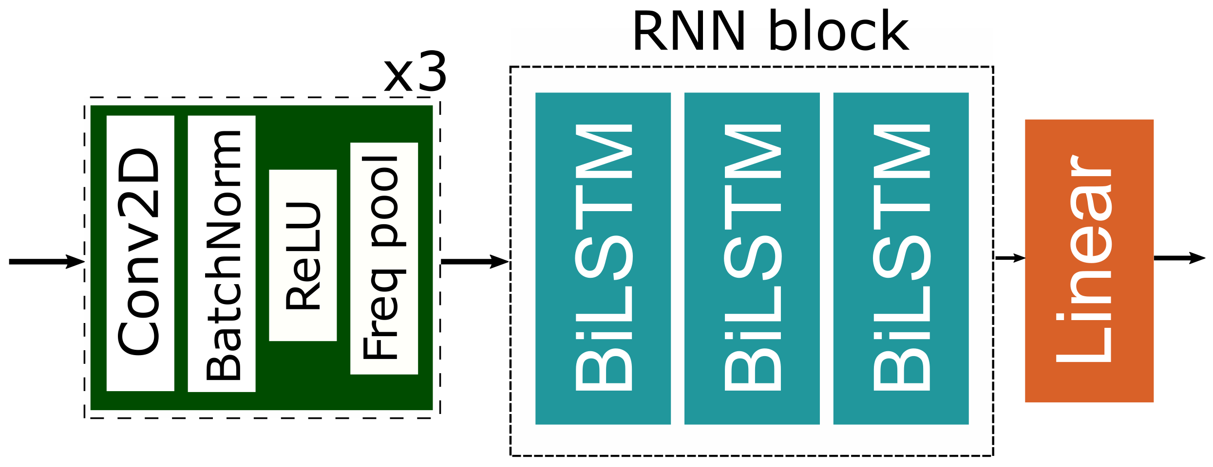
3.3. Neural Network Model

As the main element for the SAD system we opt for a CRNN based classifier. Particularly, we use the variant using 2D convolutions from the models already presented in our previous work [23]. The schematic representation of the proposed CRNN model is described in Figure 3.

As it can be observed in the figure, the model is mainly composed of two elements. First, three 2D convolutional blocks are used to process input features. Each of these blocks is integrated by a 2D convolutional layer with 3 × 3 kernel size and 64 filters. Then, it is followed by a batch normalisation layer [70] and the application of a rectified linear unit (ReLU) [71] activation function. Finally, a max-pooling mechanism is applied considering a 4 × 1 stride, so that only the frequency axis is downsampled. Then the output of the last convolutional block is fed to the RNN block, generated by stacking three bidirectional LSTM layers with 128 neurons each. This block is then followed by a linear layer that generates the speech class score as a single neuron output.

3.4. Evaluation Metrics

Two possible errors can be considered when dealing with SAD systems: a false positive (FP), this is the identification of speech in a segment where the reference identifies non-speech, and a false negative (FN), this is the missed identification of speech in a segment where the reference identifies speech. Using these two errors, the false positive rate (FPR) and false negative rate (FNR) can be computed according to the following equations:

$$\mathrm{FPR}=\frac{{\mathrm{T}}_{\mathrm{FP}}}{{\mathrm{T}}_{\mathrm{non-speech}}},$$

(12)

$$\mathrm{FNR}=\frac{{\mathrm{T}}_{\mathrm{FN}}}{{\mathrm{T}}_{\mathrm{speech}}},$$

(13)

where ${\mathrm{T}}_{\mathrm{FP}}$ and ${\mathrm{T}}_{\mathrm{FN}}$ are, respectively, the total false positive time and total false negative time for the SAD hypothesis, ${\mathrm{T}}_{\mathrm{non-speech}}$ represents the total annotated non-speech time in the reference, and ${\mathrm{T}}_{\mathrm{speech}}$ represents the total annotated speech time in the reference. Following the evaluation protocol originally proposed in the Fearless Steps Challenge [72], results are reported according to the detection cost function (DCF), as shown in the following equation:

$$\mathrm{DCF}=0.75·\mathrm{FNR}+0.25·\mathrm{FPR}.$$

(14)

As it can be observed, false negative errors were considered more important than false positive errors in the original evaluation. In addition to FPR, FNR and DCF, which are metrics depending on the chosen threshold, results of the system are also reported using the area under the ROC curve (AUC) metric, measuring the area underneath the entire receiver operating characteristics (ROC) curve, and the equal error rate (EER), the error rate at which the FNR and FPR is equal. Both metrics provide an overall measurement of performance for all the possible threshold applied to the neural networks scores. Furthermore, the desegregated performance for all possible operating points is described using the detection error trade-off (DET) curve, showing FPR values versus FNR values.

4. Results

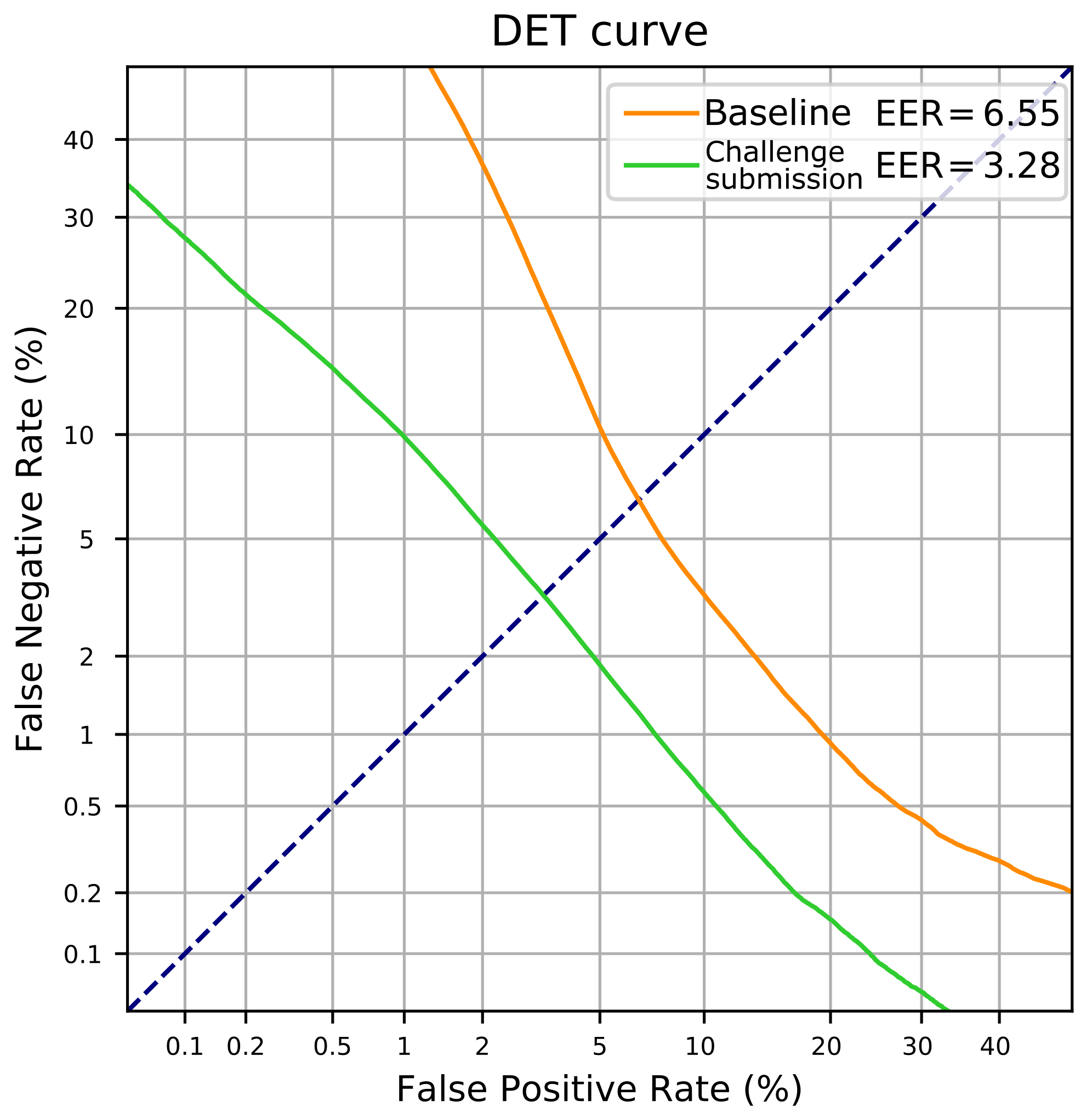
4.1. Baseline System

As starting point for the experimentation, the main objective is to obtain a baseline system so that further experiments could be compared against. This baseline model is the one considered as the unadapted model, trained only with out of domain data. This model is fine tuned in the following experiments using the methods previously explained in order to obtain a model adapted to the unseen domain. The experimental setup is built upon the description provided in Section 3. Concerning the details of the optimisation process, adam optimiser is used with a learning rate that decays exponentially from ${10}^{-3}$ to ${10}^{-4}$ during 20 epochs. Minibatch size is chosen to maximise the GPU memory usage. Model selection is performed by choosing the best performing model in terms of frame classification accuracy on the validation subset. Unless stated otherwise, these optimisation details are common among all the following experiments described in this paper.

Results for the baseline system trained on broadcast, telephonic and meetings domains in terms of AUC and EER can be observed in

Table 2. AUC (%) and EER (%) on three in domain datasets and FS02 development partition compared to a system submitted to the challenge rained using only data from FS challenge.

Model	Train Domain	Test Domain	Dataset	AUC (%)	EER (%)
Baseline	Broad. + Tele. + Meet.	Broadcast	Albayzín 2020	98.12	6.68
		Telephonic	CALLHOME	96.70	7.62
		Meetings	RT09	97.07	6.98
Baseline	Broad. + Tele. + Meet.	Apollo missions	FS02-Dev	97.57	6.55
Challenge submission	Apollo missions	Apollo missions		99.56	3.28

. Additionally, we also report the results of one of our submissions to the original FS02 challenge [23] that was trained using the same experimental setup but with data coming from the training partition provided for the challenge. This result is presented in order to provide an upper bound for the neural architecture performance in case it was trained with in domain data.

First, we report results for the three domains that the SAD baseline system has seen in the training process. In general terms, it can be observed that competitive results are obtained on the three domains shown, with EER values in the range 6 to 7%. Focusing on the obtained results for FS02 development partition, it can be observed that, as expected, the baseline system underperforms when compared to the challenge submission trained within domain data. Particularly, a drop in performance close to 50% can be observed in terms of EER. In the following subsections, we aim to fill the gap between the baseline model and the upper bound provided by the system submitted to FS challenge by using unsupervised domain adaptation techniques.

Results shown in Table 2 are complemented with those presented in Figure 4. In this figure, we show the DET curve and EER for the baseline system and the challenge submission system on FS02 development partition.

As it can be observed, a similar drop in performance measured by the EER metric is applicable to all points in DET curve. Furthermore, the baseline system tends to provide higher FNR values, whereas the challenge submission curve shows a relatively constant slope in all the displayed range. As a point for comparison, for $\mathrm{FPR}=1\%$, the challenge submission provides $\mathrm{FNR}=10\%$ while the baseline unadapted system yields FNR greater than 50%.

Now that the baseline system has been appropriately characterised and set in context, in the following subsections we present the results for the three domain adaptation techniques described in the paper.

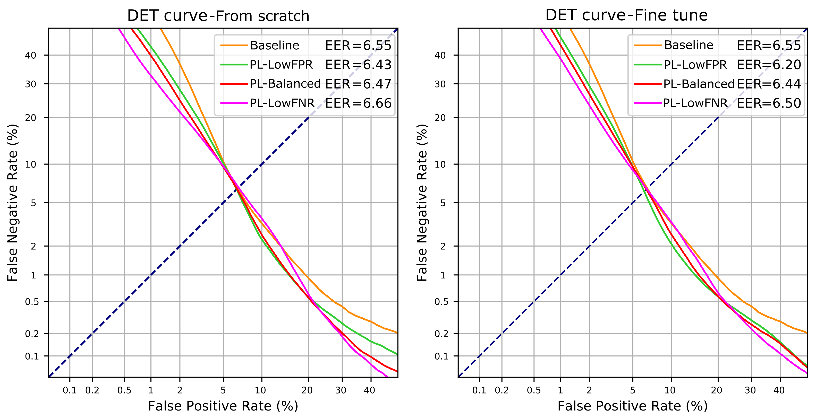
4.2. Pseudo-Label Domain Adaptation

As described in Section 2.3.1, pseudo-labelling is a method traditionally used to alleviate the need for labelled data. In the following experiments, we use it in order to adapt a model to a new unseen domain. The first step needed to perform this technique is to obtain a new set of pseudo-labels for the target data. To do so, we run the FS02 training partition through the previously obtained baseline SAD model and store the speech scores, that are then thresholded accordingly to obtain the final pseudo-labels. In the next step, those pseudo-labels are considered as the ground truth for the target data and used to train a new model in a supervised way.

Even though labels for FS02 training partition data are not used in this paper to train any model, those labels are still available and can be used to obtain an objective evaluation of the pseudo-labels obtained via the baseline model. This evaluation is shown in

Table 3. AUC, EER, FPR and FNR on three operating points for the pseudo-labels obtained using the baseline model on FS02 training partition.

Dataset	AUC (%)	EER (%)	Operating Point	FPR (%)	FNR (%)
FS02–Train	97.36	7.28	Low FPR	5.78	10.00
			Balanced	7.37	7.15
			Low FNR	11.04	3.56

in terms of AUC and EER. Furthermore, as this method relies heavily on the operating point chosen for the pseudo-labels, we also report FPR and FNR for three operating points: one with low FPR, one with balanced FPR and FNR, and one with low FNR. By using these operating points, three sets of pseudo-labels are obtained. Experiments are performed separately for each set of pseudo-labels in order to observe the influence of the operating point in this domain adaptation strategy.

As it can be observed, the values for AUC and EER are in line with those obtained with the baseline model on the development partition, yet the EER is slightly greater for the training partition. Concerning the operating points considered, it should be noted that, in general terms, by using these pseudo-labels the neural network is dealing with an approximately 15% of wrong labels in the adaptation process.

Once pseudo-labels have been obtained using the baseline model, several alternatives can be used to obtain a new adapted model. In this paper, we explore two of those alternatives. On the one hand, we train a new model from scratch using the same experimental setup as the one described for the baseline model but using FS02 training partition audio and the obtained pseudo-labels as ground-truth. On the other hand, we also evaluate the possibility of fine-tuning the baseline model via the obtained pseudo-labels for the FS02 training partition, using a learning rate ten times smaller than the one used in the original training process.

Table 4. AUC (%) and EER (%) for FS02 development partition using the pseudo-label domain transfer setup training a new neural network from scratch and fine tuning the baseline neural network.

Pseudo-Labels	From Scratch		Fine Tuning
	AUC (%)	EER (%)	AUC (%)	EER (%)
Low FPR	98.06	6.43	98.03	6.20
Balanced	98.21	6.47	98.09	6.44
Low FNR	98.26	6.66	98.19	6.50

describes the obtained results in terms of AUC and EER for each possible operating point and for both training strategies.

When compared to the unadapted baseline system, it can be observed that the results presented using the pseudo-labelling method share two common characteristics: a minor improvement in terms of AUC metrics, while the EER remains similar to the one reported in the baseline system. No significant difference can be observed between the two training strategies presented. Concerning the operating points for the pseudo-labels, the low FPR operating point yields the lowest EER for both training strategies, while at the same time also reporting the lowest AUC values.

In order to further understand the behaviour of the pseudo-labelling strategy, Figure 5 shows the DET curve and EER on the FS02 development partition for the baseline system and the systems trained using pseudo-labelling domain adaptation methods.

From Figure 5, it can be seen that the pseudo-labelling technique provides no significant improvement in EER values. On the other hand, we can see that the improvement in AUC metric observed previously comes from the improvement compared to the baseline system in DET curve in the areas with high FPR and FNR values. In general terms, experimental results suggest that pseudo-labelling techniques can help obtaining a DET curve with constant slope, reducing error in areas with high FPR and FNR values, while not significantly modifying the EER value of the system used to obtain pseudo-labels.

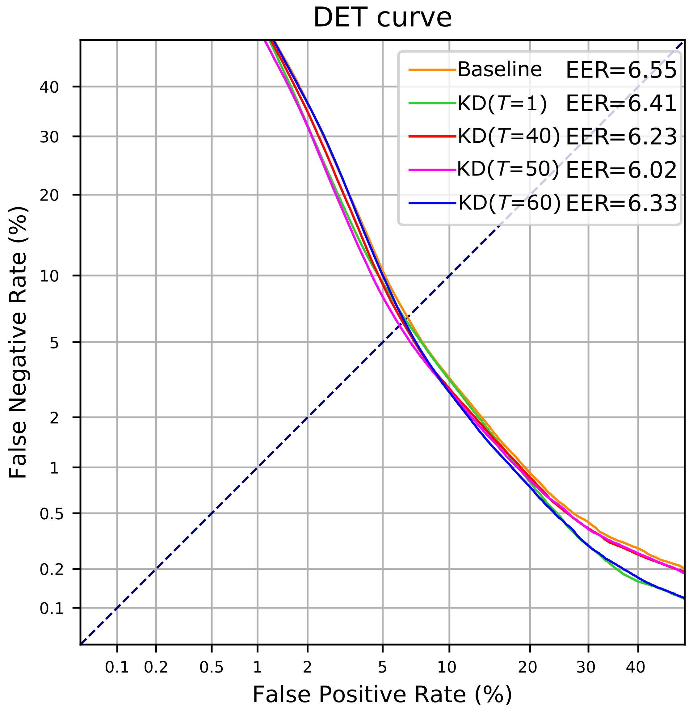
4.3. Knowledge Distillation Domain Adaptation

According to the theoretical explanation provided in Section 2.3.2, we aim to perform domain adaptation using the knowledge distillation framework applied to the SAD task. In the following, we describe the training process. First, teacher and student models are initialised using the unadapted baseline model. Teacher model weights are frozen during the entire training, and only student model weights are updated. The output of both models is compared using KLD loss after going through softmax activation with a temperature parameter T, shared for teacher and student models. At inference, the softmax layer is used in its standard form with temperature $T=1$. Obtained results in terms of AUC and EER using knowledge distillation are shown in

Table 5. AUC (%) and EER (%) on the FS02 development partition using knowledge distillation domain adaptation setup with various softmax temperature values compared to the baseline system.

Softmax Temperature	AUC (%)	EER (%)
$T=1$	97.79	6.41
$T=10$	97.72	6.32
$T=20$	97.80	6.27
$T=30$	97.80	6.25
$T=40$	97.72	6.23
$\mathit{T}=\mathbf{50}$	97.86	6.02
$T=60$	97.70	6.33

for various values of the temperature parameter T.

A decreasing tendency for EER can be observed when increasing the temperature parameter up to $T=50$, achieving a best EER value of 6.05%. However, this tendency is not consistent for the AUC metric, showing values in between 97.80 and 97.86. When compared to the baseline system, best temperature configuration reports a 8.10% relative improvement on the EER value, yet this improvement in EER only leads to a 0.29% relative improvement on the AUC metric. In general terms, an improvement in performance can be observed using the temperature softmax activation as argued by [51], however this improvement is limited.

Results in Table 5 are complemented with those presented in Figure 6. In this Figure, we present the DET curve and EER for some of the best performing knowledge distillation systems compared to the unadapted baseline system.

As observed in Figure 6, unlike the pseudo-labelling strategy, knowledge distillation seems to be able to decrease the EER point on the DET curve by using a large temperature parameter. However, it can also be seen that all curves are very close to each other; this is translated in AUC values very similar to those obtained by the baseline system. In general terms, it can also be observed that knowledge distillation does not correct the baseline system tendency to provide high FNR values. This may be due to the fact that KLD loss makes the student network mimic the predictions of the teacher network, so probability distributions and the relations between speech and non-speech observations should remain similar.

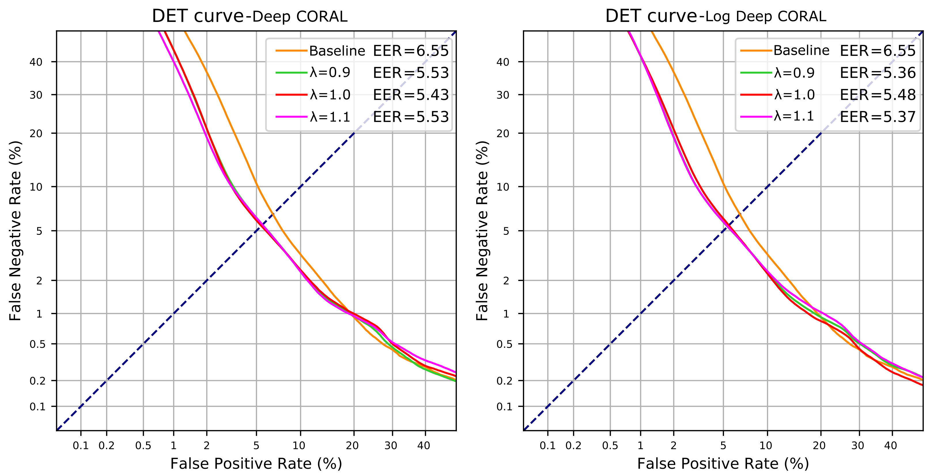
4.4. Deep CORAL Domain Adaptation

As an additional third alternative to the previously evaluated unsupervised domain adaptation techniques, in the following lines, we evaluate experimentally the feasibility of Deep CORAL and its variations for the SAD task. Following the theoretical explanation provided in Section 2.3.3, we train a new model using the Deep CORAL and Log Deep CORAL techniques using the same experimental setup: the baseline model is used to initialise the new adapted model, that is then fine tuned for 10 epochs using a learning rate decaying exponentially from ${10}^{-4}$ to ${10}^{-5}$ (10 times smaller than the one used to train the baseline model). CORAL and log CORAL losses are applied only on the final linear layer of the DNN classifier. Final loss term is then computed using cross entropy loss considering the source labels, and the respective CORAL loss weighted by a factor $\lambda$. As described in the original paper, $\lambda$ value was chosen so that, at the end of the training, the classification loss and the CORAL loss are in the same order of magnitude. Obtained results using both, Deep and Log Deep CORAL methods, are shown in

Table 6. AUC (%) and EER (%) for FS02 development partition using Deep CORAL and Log Deep CORAL domain adaptation setups using various $\lambda$ weights.

Method	CORAL Weight	AUC (%)	EER (%)
Deep CORAL	$\mathit{\lambda }\mathbf{=}\mathbf{0.9}$	98.19	5.53
	$\mathit{\lambda }\mathbf{=}\mathbf{1.0}$	98.18	5.43
	$\mathit{\lambda }\mathbf{=}\mathbf{1.1}$	98.25	5.53
Log Deep CORAL	$\mathit{\lambda }\mathbf{=}\mathbf{0.9}$	98.26	5.36
	$\mathit{\lambda }\mathbf{=}\mathbf{1.0}$	98.26	5.48
	$\mathit{\lambda }\mathbf{=}\mathbf{1.1}$	98.24	5.37

in terms of AUC and EER for three $\lambda$ values in the same order of magnitude.

As observed in Table 6, both Deep CORAL and Log Deep CORAL provide the lowest EER values obtained in this work so far through model adaptation. Best result in terms of EER is obtained using Log Deep CORAL method, with an EER of 5.36%, which results in a 18.17% relative improvement when compared to the unadapted baseline system. Concerning the AUC values observed, obtained results are in line with the best performing system using the pseudo-labelling techniques, showing also better values than the knowledge distillation method. As done in previous experiments, we also report the DET curves in order to observe the behaviour of the adapted systems in all possible operating points. This curve is shown for the Deep CORAL (left) and Log Deep CORAL (right) systems in Figure 7 for multiple values of $\lambda$ compared to the DET curve of the baseline system.

As observed, CORAL-based domain adaptation techniques provide the best improvement in the DET curve so far in this paper. When compared to the baseline system, besides significantly decreasing the EER, an overall improvement can be seen in the DET curve for the areas reporting high FNR values. That is the reason why the AUC value reported increased when compared to the baseline system. Both, Deep CORAL and Log Deep CORAL, seem to be insensitive to $\lambda$ value, showing a similar performance as long as $\lambda$ remains in the same order of magnitude.

By observing the behaviour of the Log Deep Coral method and the pseudo-label strategies previously characterised, it becomes apparent that both solutions may be complementary. While the Log Deep CORAL DET curve shows no improvement over the baseline for high FPR values, the DET curve for the pseudo-labelling method obtains its best results in that area, making it the one with best performance for high FPR values over the three methods evaluated. This fact suggest that combining both methods, applying them in cascade, might provide even further improvements to the SAD neural network. This idea is evaluated experimentally in the following subsection.

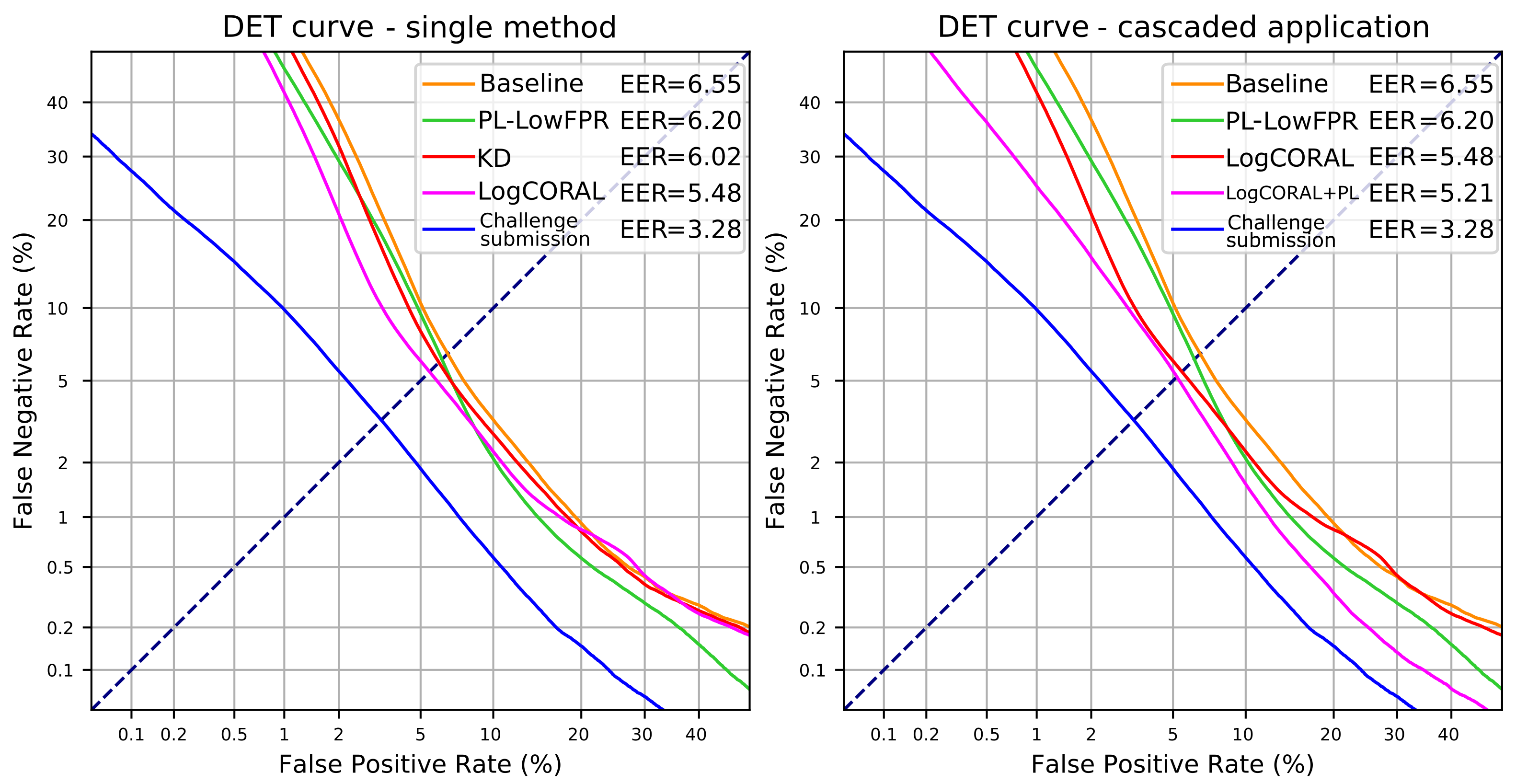
4.5. Cascaded Application of Domain Adaptation Methods

In view of results presented in previous subsections, this final experiment evaluates the possibility of applying two domain adaptation methods in a cascaded setup in order to improve even further the results on the new unseen domain. By combining the capabilities of CORAL based adaptation to obtain an overall boost in performance and the pseudo-label adaptation to obtain a DET curve with a constant slope, we use both of them in a cascaded setup. The baseline model is first adapted using the Log Deep CORAL method. Then the adapted model is used to extract a new set of pseudo-labels, which are later used to obtain a final model using both training strategies described in previous experiments, either training a new model from scratch, or fine-tuning the previous model.

Table 7. AUC, EER, FPR and FNR on three operating points for the pseudo-labels obtained using the best performing model adapted through Log Deep CORAL method on FS02 training partition.

Dataset	AUC (%)	EER (%)	Operating Point	FPR (%)	FNR (%)
FS02–Train	98.26	5.63	Low FPR	4.55	7.55
			Balanced	5.70	5.54
			Low FNR	7.27	3.78

shows an objective evaluation of the pseudo-labels obtained via the Log Deep CORAL model in terms of AUC, EER, FPR and FNR for the same three possible operating points considered in previous experiments.

As expected, we can observe that the overall quality of the pseudo-labels has improved when compared to those obtained using the baseline model (see Table 3). Improvements obtained are in line with the ones presented on the FS Development subset when using the Log Deep CORAL method, with the EER metric decreasing from 7.28 to 5.63%. By using this new set of pseudo-labels the adaptation process is performed feeding the neural network with an approximately 11% of wrong labels distributed according to the three operating points shown. Obtained results using this new set of pseudo-labels are described in

Table 8. AUC (%) and EER (%) for FS02 development partition using pseudo-label domain transfer setup training a new neural network from scratch and fine tuning the best performing model adapted using Log Deep CORAL method.

Pseudo-Labels	From Scratch		Fine Tuning
	AUC (%)	EER (%)	AUC (%)	EER (%)
Low FPR	98.86	5.21	98.85	5.34
Balanced	98.81	5.50	98.83	5.49
Low FNR	98.75	5.67	98.85	5.51

in terms of AUC and EER for each possible operating point and for both training strategies described.

The previously observed behaviour of the pseudo-labelling method is repeated in this new experiment. In general terms, compared to Log Deep CORAL model ($\mathrm{AUC}=98.25\%$, $\mathrm{EER}=5.48\%$), it can be seen that pseudo-labelling strategies provide an improvement on the AUC metric while maintaining a similar EER value. As a matter of fact, all the AUC values reported outperform those from previous experiments, with the best case scenario of $\mathrm{AUC}=98.86\%$ obtained by training a new model from scratch using low FPR pseudo-labels. Concerning the training strategies considered, experimental results suggest that no significant difference can be found between training a new model from scratch or fine tuning the previous stage model. In terms of operating point, the EER value obtained using low FPR is slightly lower for both training strategies, however this difference becomes insignificant when considering the AUC metric.

4.6. Discussion

Once all the results for the unsupervised domain adaptation methods have been described, in this subsection we aim to provide a brief discussion on its behaviour, setting them in the context of the original FS challenge and using the original DCF metric in order to obtain a performance comparison.

Table 9. AUC (%), EER (%), DCF (%) and DCF relative improvement (%) over the unadapted baseline model on the FS02 development partition using the three evaluated domain adaptation methods, and the cascaded application of two of them with the best performing hyperparameter configuration in terms of DCF metric compared to the original challenge baseline and our submission to the challenge trained using in domain data.

Model	AUC (%)	EER (%)	DCF (%)	Rel. Improv. (%)
Baseline	97.57	6.55	4.84	-
Pseudo-labels (fine tune)	98.03	6.20	4.25	12.19
Pseudo-labels (scratch)	98.21	6.46	4.31	10.95
Knowledge distillation ($T=1$)	97.79	6.41	4.78	1.24
Knowledge distillation ($T=50$)	97.86	6.02	4.56	5.79
Deep CORAL ($\lambda =1.1$)	98.25	5.53	4.26	11.98
Log Deep CORAL ($\lambda =1.0$)	98.25	5.48	4.20	13.23
Log CORAL + PL (fine tune)	98.85	5.34	3.67	24.17
Log CORAL + PL (scratch)	98.86	5.21	3.65	24.59
Challenge baseline	-	-	12.50	-
Challenge submission	99.56	3.28	2.56	-

presents a summary of the best obtained results using all methods explored (pseudo-labels, KD, Deep CORAL), and the cascaded application of both of them in terms of AUC, EER and DCF metrics as used in the FS challenge. We also report the relative improvement obtained in DCF metric compared to the unadapted baseline system. For comparison, we present the challenge baseline result provided by the FS challenge organisation [72], and our submission to the challenge trained using in domain data.

Concerning the results of the pseudo-labelling strategy, we can observe a relative improvement in DCF metric between 11% and 12% when compared to the unadapted baseline system. This improvement comes mainly from the correction made to the DET curve, with those systems showing a behaviour with more constant slope. This means that systems adapted using this method show a better performance in areas with high FPR or high FNR while, at the same time, EER remains very similar to that of the baseline system. The knowledge distillation systems offer the lowest improvement in DCF of all methods evaluated. Even though its configuration with high softmax temperature still shows a non-neglectable 5.79% relative improvement compared to the baseline system, this solution shows limited applications. DET curve is really similar to the one obtained by the baseline system, with limited improvement in AUC. Finally, CORAL-based methods show one of the most promising results of this study. The best hyperparameter configuration using Log Deep CORAL achieves a DCF relative improvement of 13.23% compared to the baseline system. These results shows the lowest EER value in this paper in the case of the application of a single technique, while also reporting an overall improvement for the full DET curve.

Best results in terms of DCF are obtained by applying Log Deep CORAL and pseudo-labelling in a cascaded setup. In the case of training a new model from scratch using pseudo-labels from the previous step, DCF is 3.65%, which is equivalent to 24.59% relative improvement compared to the unadapted baseline system. Furthermore, experimental results confirm that both methods are complementary. As shown, the total relative improvement with both techniques is equivalent to the sum of relative improvements when used separately.

As a final point in this discussion, and in order to provide a condensed view of the best obtained results in this work, Figure 8 presents DET curve and EER of the three evaluated methods by themselves (left), and the cascaded application of Log Deep CORAL and pseudo-labelling (right) using the best hyperparameter configuration in terms of DCF metric compared to the unadapted baseline and our submission to the challenge trained using in domain data.

Observing the comparative of the single method application (left), it can be seen again that the most promising result in terms of improving the DET curve is obtained by the Log Deep CORAL method, while the improvement of the knowledge distillation method is limited. Focusing on the comparison on the cascaded application of Deep CORAL and pseudo-labelling (right), it can be observed that the DET curve obtained for the cascaded application of both methods (in pink) supports again the hypothesis that both techniques are complementary. Applying the pseudo-labelling strategy on top of the Log Deep CORAL model results in a DET curve with a similar EER value but a performance significantly improved in areas with high FPR and high FNR. With this method we achieve the best DET curve in this paper that, as already presented, allows to decrease even further the DCF metric, which is influenced in a higher way by false negative errors. As an example operating point for comparison, focusing on a FPR value of 1%, the unadapted baseline system shows a FNR value greater than 50%. While the Log Deep CORAL model reduces this value to be approximately 40%, the improvement is much more significant with the combination of both adaptation methods, that reports a FNR value of 25%.

Even though there is still a gap between the best obtained results and a model trained using in domain data, in practical scenarios, where no labels are available, experimental results have proved that unsupervised domain adaptation can improve significantly the performance of SAD systems. Best results are obtained using an approach that combines two methods. The application of this solution increases the computational complexity of the adaptation process in training time. However, the increase in complexity introduced by pseudo-labelling is minimal compared to the one already introduced by Log Deep CORAL. The latter implies a training process that computes two covariance matrices for CORAL loss and a classification loss, while the former only requires inference computation on the unlabelled data and then a simple training process with a classification loss. Furthermore, inference complexity remains the same in all cases as there is only need to compute the final adapted model to obtain SAD predictions.

5. Conclusions and Future Lines

In this paper, we have explored the use of unsupervised domain adaptation techniques in the context of the SAD task. An initial baseline model was trained on a variety of well-known domains with big amounts of labelled data available. Then, a study was performed on three methods that allow to perform adaptation directly on the model space with the objective of fine tuning the mentioned baseline model using only unlabelled data. We have used the data provided in the FS challenge, coming from a singular domain such as Apollo space missions, to experimentally validate in the SAD task the methods presented. Yet, the methods are general enough so that they can be easily applied to other datasets. Furthermore, no labels are required for them to be used, significantly reducing the constraints for choosing them in practical applications.

Through the application of Deep CORAL based domain adaptation methods, results show a 13% relative improvement in DCF metric of the original challenge. Furthermore, the cascaded application of Deep CORAL and pseudo-labelling techniques provides the best results in this study, with a significant 24% relative improvement compared to the baseline system. These experimental results suggest that Deep CORAL and pseudo-labelling techniques are complementary. The first one providing an overall improvement in the DET curve and reducing the EER. The second one improves the AUC value by modifying the DET curve so that its slope becomes constant, specially in areas with high FPR and FNR values. The improvements in performance observed allow to substantially reduce the gap for the SAD task between a system trained using in domain data and an approach based on fully unsupervised adaptation.

Even if the knowledge distillation method shows an improvement in performance compared to the unadapated baseline model, this improvement is limited compared to the one observed by CORAL based techniques. This kind of domain adaptation methods, seeking to minimise the statistical distribution shift between source and target domains, provide one of the most promising results in this paper. Some recent work has introduced the use of higher-order statistics for unsupervised domain adaptation [73], generalising the idea presented in Deep CORAL as an arbitrary order moment matching technique. Some of our future work lines may point in this direction, applying this idea to the SAD task.

References

1. Gerven, S.V.; Xie, F. A comparative study of speech detection methods. In Proceedings of the Fifth European Conference on Speech Communication and Technology, Rhodes, Greece, 22–25 September 1997. [Google Scholar]
2. Junqua, J.C.; Mak, B.; Reaves, B. A robust algorithm for word boundary detection in the presence of noise. IEEE Trans. Speech Audio Process. 1994, 2, 406–412. [Google Scholar] [CrossRef]
3. Chang, J.H.; Kim, N.S.; Mitra, S.K. Voice activity detection based on multiple statistical models. IEEE Trans. Signal Process. 2006, 54, 1965–1976. [Google Scholar] [CrossRef]
4. Ng, T.; Zhang, B.; Nguyen, L.; Matsoukas, S.; Zhou, X.; Mesgarani, N.; Veselỳ, K.; Matějka, P. Developing a Speech Activity Detection system for the DARPA RATS program. In Proceedings of the Interspeech, Portland, OR, USA, 9–13 September 2012; pp. 1969–1972. [Google Scholar]
5. Woo, K.H.; Yang, T.Y.; Park, K.J.; Lee, C. Robust voice activity detection algorithm for estimating noise spectrum. Electron. Lett. 2000, 36, 180–181. [Google Scholar] [CrossRef]
6. Ramırez, J.; Segura, J.C.; Benıtez, C.; De La Torre, A.; Rubio, A. Efficient voice activity detection algorithms using long-term speech information. Speech Commun. 2004, 42, 271–287. [Google Scholar] [CrossRef]
7. Liu, B.; Wang, Z.; Guo, S.; Yu, H.; Gong, Y.; Yang, J.; Shi, L. An energy-efficient voice activity detector using deep neural networks and approximate computing. Microelectron. J. 2019, 87, 12–21. [Google Scholar] [CrossRef]
8. Vesperini, F.; Vecchiotti, P.; Principi, E.; Squartini, S.; Piazza, F. Deep neural networks for multi-room voice activity detection: Advancements and comparative evaluation. In Proceedings of the 2016 International Joint Conference on Neural Networks (IJCNN), Vancouver, BC, Canada, 24–29 July 2016; pp. 3391–3398. [Google Scholar]
9. Fan, Z.C.; Bai, Z.; Zhang, X.L.; Rahardja, S.; Chen, J. AUC Optimization for Deep Learning Based Voice Activity Detection. In Proceedings of the IEEE ICASSP, Brighton, UK, 12–17 May 2019; pp. 6760–6764. [Google Scholar]
10. Hochreiter, S.; Schmidhuber, J. Long short-term memory. Neural Comput. 1997, 9, 1735–1780. [Google Scholar] [CrossRef]
11. Kim, J.; Kim, J.; Lee, S.; Park, J.; Hahn, M. Vowel based voice activity detection with LSTM recurrent neural network. In Proceedings of the 8th International Conference on Signal Processing Systems, Auckland, New Zealand, 21–24 November 2016; pp. 134–137. [Google Scholar]
12. de Benito-Gorron, D.; Lozano-Diez, A.; Toledano, D.T.; Gonzalez-Rodriguez, J. Exploring convolutional, recurrent, and hybrid deep neural networks for speech and music detection in a large audio dataset. EURASIP J. Audio Speech Music Process. 2019, 2019, 9. [Google Scholar] [CrossRef] [Green Version]
13. Viñals, I.; Gimeno, P.; Ortega, A.; Miguel, A.; Lleida, E. Estimation of the Number of Speakers with Variational Bayesian PLDA in the DIHARD Diarization Challenge. In Proceedings of the Interspeech, Hyderabad, India, 2–6 September 2018; pp. 2803–2807. [Google Scholar]
14. Vinals, I.; Gimeno, P.; Ortega, A.; Miguel, A.; Lleida, E. In-domain Adaptation Solutions for the RTVE 2018 Diarization Challenge. In Proceedings of the IberSPEECH, Barcelona, Spain, 21–23 November 2018; pp. 220–223. [Google Scholar]
15. Sainath, T.N.; Vinyals, O.; Senior, A.; Sak, H. Convolutional, long short-term memory, fully connected deep neural networks. In Proceedings of the 2015 IEEE International Conference on Acoustics, Speech and Signal Processing (ICASSP), South Brisbane, QLD, Australia, 19–24 April 2015; pp. 4580–4584. [Google Scholar]
16. Huang, X.; Qiao, L.; Yu, W.; Li, J.; Ma, Y. End-to-end sequence labeling via convolutional recurrent neural network with a connectionist temporal classification layer. Int. J. Comput. Intell. Syst. 2020, 13, 341–351. [Google Scholar] [CrossRef] [Green Version]
17. Vafeiadis, A.; Fanioudakis, E.; Potamitis, I.; Votis, K.; Giakoumis, D.; Tzovaras, D.; Chen, L.; Hamzaoui, R. Two-Dimensional Convolutional Recurrent Neural Networks for Speech Activity Detection. In Proceedings of the Interspeech 2019, Graz, Austria, 15–19 September 2019; pp. 2045–2049. [Google Scholar] [CrossRef] [Green Version]
18. Byers, F.; Byers, F.; Sadjadi, O. 2017 Pilot Open Speech Analytic Technologies Evaluation (2017 NIST Pilot OpenSAT): Post Evaluation Summary; US Department of Commerce, National Institute of Standards and Technology: Gaithersburg, MD, USA, 2019.
19. Hansen, J.H.; Joglekar, A.; Shekhar, M.C.; Kothapally, V.; Yu, C.; Kaushik, L.; Sangwan, A. The 2019 Inaugural Fearless Steps Challenge: A Giant Leap for Naturalistic Audio. In Proceedings of the Interspeech, Graz, Austria, 15–19 September 2019; pp. 1851–1855. [Google Scholar]
20. Hansen, J.H.; Sangwan, A.; Joglekar, A.; Bulut, A.E.; Kaushik, L.; Yu, C. Fearless Steps: Apollo-11 Corpus Advancements for Speech Technologies from Earth to the Moon. In Proceedings of the Interspeech, Hyderabad, India, 2–6 September 2018; pp. 2758–2762. [Google Scholar]
21. Mezza, A.I.; Habets, E.A.; Müller, M.; Sarti, A. Unsupervised domain adaptation for acoustic scene classification using band-wise statistics matching. In Proceedings of the 2020 28th European Signal Processing Conference (EUSIPCO), Virtual, 18–22 January 2021; pp. 11–15. [Google Scholar]
22. Anoop, C.; Prathosh, A.; Ramakrishnan, A. Unsupervised domain adaptation schemes for building ASR in low-resource languages. In Proceedings of the Workshop on Automatic Speech Recognition and Understanding, ASRU, Cartagena, Colombia, 15–17 December 2021. [Google Scholar]
23. Gimeno, P.; Ribas, D.; Ortega, A.; Miguel, A.; Lleida, E. Convolutional recurrent neural networks for Speech Activity Detection in naturalistic audio from apollo missions. Proc. IberSPEECH 2021, 2021, 26–30. [Google Scholar]
24. Gimeno, P.; Ortega, A.; Miguel, A.; Lleida, E. Unsupervised Representation Learning for Speech Activity Detection in the Fearless Steps Challenge 2021. In Interspeech 2021; ISCA: Singapore, 2021; pp. 4359–4363. [Google Scholar]
25. Zhang, X.L. Unsupervised domain adaptation for deep neural network based voice activity detection. In Proceedings of the 2014 IEEE International Conference on Acoustics, Speech and Signal Processing (ICASSP), Florence, Italy, 4–9 May 2014; pp. 6864–6868. [Google Scholar]
26. Luo, Y.; Zheng, L.; Guan, T.; Yu, J.; Yang, Y. Taking a closer look at domain shift: Category-level adversaries for semantics consistent domain adaptation. In Proceedings of the IEEE/CVF Conference on Computer Vision and Pattern Recognition, Long Beach, CA, USA, 15–20 June 2019; pp. 2507–2516. [Google Scholar]
27. Chu, C.; Wang, R. A survey of domain adaptation for neural machine translation. arXiv 2018, arXiv:1806.00258. [Google Scholar]
28. Wilson, G.; Cook, D.J. A survey of unsupervised deep domain adaptation. ACM Trans. Intell.Syst. Technol. 2020, 11, 1–46. [Google Scholar] [CrossRef] [PubMed]
29. Sun, S.; Zhang, B.; Xie, L.; Zhang, Y. An unsupervised deep domain adaptation approach for robust speech recognition. Neurocomputing 2017, 257, 79–87. [Google Scholar] [CrossRef]
30. Wang, Q.; Rao, W.; Sun, S.; Xie, L.; Chng, E.S.; Li, H. Unsupervised domain adaptation via domain adversarial training for speaker recognition. In Proceedings of the 2018 IEEE International Conference on Acoustics, Speech and Signal Processing (ICASSP), Calgary, AB, Canada, 15–20 April 2018; pp. 4889–4893. [Google Scholar]
31. Mavaddaty, S.; Ahadi, S.M.; Seyedin, S. A novel speech enhancement method by learnable sparse and low-rank decomposition and domain adaptation. Speech Commun. 2016, 76, 42–60. [Google Scholar] [CrossRef]
32. Wang, M.; Deng, W. Deep visual domain adaptation: A survey. Neurocomputing 2018, 312, 135–153. [Google Scholar] [CrossRef] [Green Version]
33. Tan, B.; Zhang, Y.; Pan, S.; Yang, Q. Distant domain transfer learning. In Proceedings of the AAAI Conference on Artificial Intelligence, San Francisco, CA, USA, 4–9 February 2017; Volume 31. [Google Scholar]
34. Csurka, G. Domain adaptation for visual applications: A comprehensive survey. arXiv 2017, arXiv:1702.05374. [Google Scholar]
35. Hu, J.; Lu, J.; Tan, Y.P. Deep transfer metric learning. In Proceedings of the IEEE Conference on Computer Vision and Pattern Recognition, Boston, MA, USA, 1–7 June 2015; pp. 325–333. [Google Scholar]
36. Long, M.; Zhu, H.; Wang, J.; Jordan, M.I. Unsupervised domain adaptation with residual transfer networks. arXiv 2016, arXiv:1602.04433. [Google Scholar]
37. Sun, B.; Feng, J.; Saenko, K. Return of frustratingly easy domain adaptation. In Proceedings of the AAAI Conference on Artificial Intelligence, Phoenix, AZ, USA, 12–17 February 2016; Volume 30. [Google Scholar]
38. Li, Y.; Wang, N.; Shi, J.; Liu, J.; Hou, X. Revisiting batch normalization for practical domain adaptation. arXiv 2016, arXiv:1603.04779. [Google Scholar]
39. Liu, M.Y.; Tuzel, O. Coupled generative adversarial networks. Adv. Neural Inf. Process. Syst. 2016, 29, 469–477. [Google Scholar]
40. Ganin, Y.; Ustinova, E.; Ajakan, H.; Germain, P.; Larochelle, H.; Laviolette, F.; Marchand, M.; Lempitsky, V. Domain-adversarial training of neural networks. J. Mach. Learn. Res. 2016, 17, 2030–2096. [Google Scholar]
41. Zhuang, F.; Cheng, X.; Luo, P.; Pan, S.J.; He, Q. Supervised representation learning: Transfer learning with deep autoencoders. In Proceedings of the Twenty-Fourth International Joint Conference on Artificial Intelligence, Buenos Aires, Argentina, 25–31 July 2015. [Google Scholar]
42. Zhu, J.Y.; Park, T.; Isola, P.; Efros, A.A. Unpaired image-to-image translation using cycle-consistent adversarial networks. In Proceedings of the IEEE International Conference on Computer Vision, Venice, Italy, 22–29 October 2017; pp. 2223–2232. [Google Scholar]
43. Lee, D.H. Pseudo-label: The simple and efficient semi-supervised learning method for deep neural networks. Workshop Chall. Represent. Learn. ICML 2013, 3, 896. [Google Scholar]
44. Iscen, A.; Tolias, G.; Avrithis, Y.; Chum, O. Label propagation for deep semi-supervised learning. In Proceedings of the IEEE/CVF Conference on Computer Vision and Pattern Recognition, Long Beach, CA, USA, 15–20 June 2019; pp. 5070–5079. [Google Scholar]
45. Shi, W.; Gong, Y.; Ding, C.; Tao, Z.M.; Zheng, N. Transductive semi-supervised deep learning using min-max features. In Proceedings of the European Conference on Computer Vision (ECCV), Munich, Germany, 8–14 September 2018; pp. 299–315. [Google Scholar]
46. Wang, G.H.; Wu, J. Repetitive reprediction deep decipher for semi-supervised learning. In Proceedings of the AAAI Conference on Artificial Intelligence, New York, NY, USA, 7–12 February 2020; Volume 34, pp. 6170–6177. [Google Scholar]
47. Rizve, M.N.; Duarte, K.; Rawat, Y.S.; Shah, M. In defense of pseudo-labeling: An uncertainty-aware pseudo-label selection framework for semi-supervised learning. arXiv 2021, arXiv:2101.06329. [Google Scholar]
48. Zhong, M.; LeBien, J.; Campos-Cerqueira, M.; Dodhia, R.; Ferres, J.L.; Velev, J.P.; Aide, T.M. Multispecies bioacoustic classification using transfer learning of deep convolutional neural networks with pseudo-labeling. Appl. Acoust. 2020, 166, 107375. [Google Scholar] [CrossRef]
49. Takashima, Y.; Fujita, Y.; Horiguchi, S.; Watanabe, S.; García, P.; Nagamatsu, K. Semi-Supervised Training with Pseudo-Labeling for End-to-End Neural Diarization. arXiv 2021, arXiv:2106.04764. [Google Scholar]
50. Xu, Q.; Likhomanenko, T.; Kahn, J.; Hannun, A.; Synnaeve, G.; Collobert, R. Iterative pseudo-labeling for speech recognition. arXiv 2020, arXiv:2005.09267. [Google Scholar]
51. Hinton, G.; Vinyals, O.; Dean, J. Distilling the knowledge in a neural network. arXiv 2015, arXiv:1503.02531. [Google Scholar]
52. Shen, P.; Lu, X.; Li, S.; Kawai, H. Feature Representation of Short Utterances Based on Knowledge Distillation for Spoken Language Identification. In Proceedings of the Interspeech, Hyderabad, India, 2–6 September 2018; pp. 1813–1817. [Google Scholar]
53. Li, J.; Zhao, R.; Chen, Z.; Liu, C.; Xiao, X.; Ye, G.; Gong, Y. Developing far-field speaker system via teacher-student learning. In Proceedings of the 2018 IEEE International Conference on Acoustics, Speech and Signal Processing (ICASSP), Calgary, AB, Canada, 15–20 April 2018; pp. 5699–5703. [Google Scholar]
54. Korattikara, A.; Rathod, V.; Murphy, K.; Welling, M. Bayesian dark knowledge. arXiv 2015, arXiv:1506.04416. [Google Scholar]
55. Asami, T.; Masumura, R.; Yamaguchi, Y.; Masataki, H.; Aono, Y. Domain adaptation of dnn acoustic models using knowledge distillation. In Proceedings of the 2017 IEEE International Conference on Acoustics, Speech and Signal Processing (ICASSP), New Orleans, LA, USA, 5–9 March 2017; pp. 5185–5189. [Google Scholar]
56. Li, J.; Seltzer, M.L.; Wang, X.; Zhao, R.; Gong, Y. Large-scale domain adaptation via teacher-student learning. arXiv 2017, arXiv:1708.05466. [Google Scholar]
57. Luckenbaugh, J.; Abplanalp, S.; Gonzalez, R.; Fulford, D.; Gard, D.; Busso, C. Voice Activity Detection with Teacher-Student Domain Emulation. Proc. Interspeech 2021, 2021, 4374–4378. [Google Scholar]
58. Dinkel, H.; Wang, S.; Xu, X.; Wu, M.; Yu, K. Voice activity detection in the wild: A data-driven approach using teacher-student training. IEEE/ACM Trans. Audio Speech Lang. Process. 2021, 29, 1542–1555. [Google Scholar] [CrossRef]
59. Sun, B.; Saenko, K. Deep coral: Correlation alignment for deep domain adaptation. In Proceedings of the European Conference on Computer Vision, Amsterdam, The Netherlands, 8–16 October 2016; Springer: Berlin/Heidelberg, Germany, 2016; pp. 443–450. [Google Scholar]
60. Morerio, P.; Murino, V. Correlation alignment by riemannian metric for domain adaptation. arXiv 2017, arXiv:1705.08180. [Google Scholar]
61. Huang, Z.; Gool, L.V. A Riemannian Network for SPD Matrix Learning. arXiv 2016, arXiv:1608.04233. [Google Scholar]
62. MacDuffee, C.C. The Theory of Matrices; Springer Science & Business Media: Berlin/Heidelberg, Germany, 2012; Volume 5. [Google Scholar]
63. Butko, T.; Nadeu, C. Audio segmentation of broadcast news in the Albayzin-2010 evaluation: Overview, results, and discussion. EURASIP J. Audio Speech Music Process. 2011, 2011, 1. [Google Scholar] [CrossRef] [Green Version]
64. McCowan, I.; Carletta, J.; Kraaij, W.; Ashby, S.; Bourban, S.; Flynn, M.; Guillemot, M.; Hain, T.; Kadlec, J.; Karaiskos, V.; et al. The AMI meeting corpus. In Proceedings of the 5th International Conference on Methods and Techniques in Behavioral Research, Wageningen, The Netherlands, 30 August–2 September 2005; Volume 88, p. 100. [Google Scholar]
65. Lleida, E.; Ortega, A.; Miguel, A.; Bazán-Gil, V.; Pérez, C.; Gómez, M.; De Prada, A. Albayzin 2018 evaluation: The iberspeech-rtve challenge on speech technologies for spanish broadcast media. Appl. Sci. 2019, 9, 5412. [Google Scholar] [CrossRef] [Green Version]
66. Janin, A.; Baron, D.; Edwards, J.; Ellis, D.; Gelbart, D.; Morgan, N.; Peskin, B.; Pfau, T.; Shriberg, E.; Stolcke, A.; et al. The ICSI meeting corpus. In Proceedings of the 2003 IEEE International Conference on Acoustics, Speech, and Signal Processing, Proceedings (ICASSP’03), Hong Kong, China, 6–10 April 2003; Volume 1, p. I. [Google Scholar]
67. Bell, P.; Gales, M.J.; Hain, T.; Kilgour, J.; Lanchantin, P.; Liu, X.; McParland, A.; Renals, S.; Saz, O.; Wester, M.; et al. The MGB challenge: Evaluating multi-genre broadcast media recognition. In Proceedings of the 2015 IEEE Workshop on Automatic Speech Recognition and Understanding (ASRU), Scottsdale, AZ, USA, 13–17 December 2015; pp. 687–693. [Google Scholar]
68. Ortega, A.; Miguel, A.; Lleida, E.; Bazán, V.; Pérez, C.; Gómez, M.; de Prada, A. Albayzin Evaluation: IberSPEECH-RTVE 2020 Speaker Diarization and Identity Assignment. 2020. Available online: http://catedrartve.unizar.es/reto2020/EvalPlan-SD-2020-v1.pdf (accessed on 7 February 2022).
69. Canavan, A.; Graff, D.; Zipperlen, G. Callhome American English Speech; Linguistic Data Consortium: Philadelphia, PA, USA, 1997. [Google Scholar]
70. Ioffe, S.; Szegedy, C. Batch normalization: Accelerating deep network training by reducing internal covariate shift. In Proceedings of the International Conference on Machine Learning, PMLR, Lille, France, 7–9 July 2015; pp. 448–456. [Google Scholar]
71. Nair, V.; Hinton, G.E. Rectified linear units improve restricted boltzmann machines. In Proceedings of the 27th International Conference on Machine Learning (ICML-10), Haifa, Israel, 21–24 June 2010; pp. 807–814. [Google Scholar]
72. Joglekar, A.; Hansen, J.H.; Shekar, M.C.; Sangwan, A. Fearless Steps Challenge (fs-2): Supervised learning with massive naturalistic apollo data. arXiv 2020, arXiv:2008.06764. [Google Scholar]
73. Chen, C.; Fu, Z.; Chen, Z.; Jin, S.; Cheng, Z.; Jin, X.; Hua, X.S. HoMM: Higher-order moment matching for unsupervised domain adaptation. In Proceedings of the AAAI Conference on Artificial Intelligence, New York, NY, USA, 7–12 February 2020; Volume 34, pp. 3422–3429. [Google Scholar]
Figure 1. Schematic description of the proposal for the knowledge distillation domain adaptation technique.
Applsci 12 01832 g001
Figure 2. Schematic representation of Deep CORAL adaptation technique.
Applsci 12 01832 g002
Figure 3. Convolutional recurrent neural network model proposed for the SAD task.
Applsci 12 01832 g003
Figure 4. DET curve and EER (%) on FS02 development partition comparing a baseline system trained using out of domain data and our submission to the challenge trained using in domain data.
Applsci 12 01832 g004
Figure 5. DET curve and EER (%) on the FS02 development partition using the pseudo-label domain transfer setup training a new neural network from scratch (left) and fine-tuning the baseline neural network (right), both compared to the baseline system.
Applsci 12 01832 g005
Figure 6. DET curve and EER(%) on the FS02 development partition using the knowledge distillation domain adaptation setup with various softmax temperature values compared to the baseline system.
Applsci 12 01832 g006
Figure 7. DET curve and EER (%) on the FS02 development partition using Deep CORAL (left) and Log Deep CORAL (right) domain adaptation setups using multiple λ weights compared to the baseline system.
Applsci 12 01832 g007
Figure 8. DET curve and EER(%) on the FS02 development partition using the three evaluated domain adaptation methods (left), and the cascaded application of two of them (right) with the best performing hyperparameter configuration in terms of DCF metric compared to the unadapted baseline system and our submission to the challenge trained using in domain data.
Applsci 12 01832 g008