Variational Inference for a Recommendation System in IoT Networks Based on Stein’s Identity

Abstract

The recommendation services are critical for IoT since they provide interconnection between various devices and services. In order to make Internet searching convenient and useful, algorithms must be developed that overcome the shortcomings of existing online recommendation systems. Therefore, a novel Stein Variational Recommendation System algorithm (SVRS) is proposed, developed, implemented and tested in this paper in order to address the long-standing recommendation problem. With Stein’s identity, SVRS is able to calculate the feature vectors of users and ratings it has generated, as well as infer the preference for users who have not rated certain items. It has the advantages of low complexity, scalability, as well as providing insights into the formation of ratings. A set of experimental results revealed that SVRS performed better than other types of recommendation methods in root mean square error (RMSE) and mean absolute error (MAE).

1. Introduction

The vast amount of online content will drown Internet users if online recommendation systems are not in place, and IoT developers will be confused. Therefore, a huge challenge exists in extracting useful information from vast amounts of data [1,2]. In order to help users choose what they want or need, recommendation systems have been given plenty of attention.

In order to facilitate content recommendation, researchers have developed several mechanisms. They can be classified into four categories: collaborative filtering (CF)-based (which includes latent factor models or matrix factorization), social network-based, deep learning (DL)-based and variational inference (VI)-based [3,4] (see Table 1).

Table 1. Advantages and disadvantages of different recommendation methods.

Classification	Disadvantages	Advantages
Collaborative filtering-based	High computing cost when dealing with large data, low accuracy in the existence of sparsity, difficulty to explain	Direct and intuitive to implement
Social network-based	Unstable accuracy, lacks individuality and freshness	Works well for most social networks
Content-based	Cold start and overfitting	Works well for field require professional knowledge
Deep learning-based	Require big data, only suitable for situations involving visual elements and only keyword match is not sufficient	Powerful computing ability, often more accurate
Variational inference-based	Accuracy or complexity depend on the complexity of assumptions of target density, too specific	Reduce overfitting, efficient in computing hyper-parameters

The first type of recommendation recommends by locating existing users with suitable preferences and offers the content based on their content lists. Collaborative filtering has become the widely-used recommendation approach in recent decades. The probabilistic matrix factorization (PMF) was brought up by Salakhutdinov and Mnih in 2007, for example, in order to predict Netflix user ratings. The Bayesian probabilistic matrix factorization (BPMF) proposed by Salakhutdinov and Mnih [5] uses the Markov Chain Monte Carlo (MCMC) sampling and can deal with large datasets. Based on item categories and an interesting measure, Wei et al. developed a new item-based CF recommendation algorithm in 2012 [6]. The algorithm can deal with sparsity and thus demonstrate high accuracy. The Tag-Based Recommendation System that Yin et al. presented in 2016 can output a customized recommendation list for TV users through a tag-based recommendation list [7]. A new integrated CF recommendation for social cyber physical system (CPS) was released in 2017 by Xu et al. [8]. In addition to item ratings and user ratings, the proposed algorithm also uses social trust to improve choices. On 15 March 2019, Xu et al. proposed an algorithm for determining the independent degree between different classification sets that is based on Gaussian cores [9]. In 2020, Meng et al. proposed a security-driven hybrid collaborative recommendation method for a cloud-based IoT service [10]. Even though a CF-based recommendation is simple to apply, it has a few favorable features, such as high computing costs for large user numbers and low accuracy in the existence of sparsity, as well as difficulty in explaining [11].

Since the preference of one user is influenced by the preference of another user, a social network-based recommendation is easy to understand. Thus, social network-based recommendations have both advantages and disadvantages. Generally, the recommendations are correct but lack originality and freshness [12].

The content-based recommendation method creates a user preference file from the user’s rating, viewing, and labeling behavior so that it can recommend the contents most aligned with that preference. In their pioneering paper, Basu et al. developed a recommending algorithm capable of incorporating both user ratings and item knowledge [13]. Then, Bhagavatula et al. developed the content-based academic paper recommending system [14], Pablo et al. developed an artwork recommendation based on content [15], and Sun et al. developed a customized service recommendation system based on content [16]. An algorithm based on content is obviously better for those with professional knowledge in that field. However, content-based recommendations face the issue of cold starts and overfitting.

Deep learning systems offer superior accuracy to traditional recommendation algorithms because of the computing power enabled by deep neural networks. As part of their research on DL-based recommendation systems for various uses, Song et al. brought up a method that utilizes long-term and short-term user history to boost recommendation accuracy [17]. Using neural networks to model the client’s penchant for all kinds of online content, Zheng et al. developed a neural autoregressive distribution estimator (NADE) system the following year. An image recommendation system based on DL for large scale online commerce was proposed by Shankar et al. in 2017 [18]. This process computes how similar the visual characteristics of different items are to each other and makes recommendations based on that information. An algorithm integrating DL and CF was proposed by Deng et al. [19] in 2019. Then, Fang and colleagues exploited DNN’s sequentiality to enhance recommending performance by capturing Internet users’ preferences in real time [20]. A second DLTSR-based system was developed by Bai et al. [21] in 2020. Since, in practical terms, deep neural network (DNN) models are only suitable for some scenarios that contain visual elements and for which only word searching is not sufficient, such as garment recommendation. Thus, we need other recommendation algorithms to complement the DL-based method.

The VI-based approach has become popular among researchers because it helps reduce overfitting and efficiently solves hyperparameters. A variational Bayesian matrix factorizations-based movie recommendation algorithm developed by Koenigstein et al. in 2013 is one example. Using variational Bayesian methods, Lim et al. developed a method for predicting TV program feedback. A 2015 paper by Sedhain and his colleagues [22] described an approach that utilizes autoencoders (a VI approach) with CF-based recommendation systems. In a study by Zhang et al. on deep optimization of sparse data using variational matrix factorization, they propose an algorithm for making recommendations based on a large scale sparse rating matrix [23]. Then, in 2019, Shen et al. [24] developed a recommendation system that uses both deep learning, VI, and matrix factorization, called deep variational matrix factorization (DVMF). However, the accuracy and complexity of VI depend in large part on how complex the target density is, and without full knowledge, it is difficult to construct general VI models. Thus, to use a VI model in different scenarios, we have to construct VI algorithms that improve generality [25]. Recently, Stein’s method, another class of VI method, is a general tool to obtain bounds on distances between distributions, offering a powerful density approximation solution [26].

In this paper, inspired by the generalization and low-complexity of Stein’s method, we offer a Stein Variational Recommendation System that reduces overfitting, incorporates large volumes of data, and has lower MAE and RMSE. In this paper, we develop and analyze an SVRS algorithm both theoretically and experimentally in terms of accuracy and complexity. We also provide justifications and characteristics of our SVRS in the appendix.

We discuss the concept of SVRS in Section 2, and we provide a detailed explanation of SVRS in Section 3. In Section 4, we simulate experimental comparisons of SVRS with others. In the end, the paper is concluded in Section 6.

2. Preliminaries

First, we introduce Stein’s identity, the core of SVRS. We define $p\left(u_i\right)$ as the feature of user i, $p\left(v_j\right)$ that of IoT service j, the density to be obtained, and $\varphi \left(u\right)=[{\varphi }_1\left(u\right),\cdots ,{\varphi }_d\left(u\right)]$ and $\varphi \left(v\right)=[{\varphi }_1\left(v\right),\cdots ,{\varphi }_d\left(v\right)]$, the approximate distribution or functions of $p\left(u\right)$ and $p\left(v\right)$. Stein’s discrepancy, a general measure of how different two distributions, is the basis of Stein’s identity, which means that, for any regular $\varphi$, the following equality stands:

$${\mathbb{E}}_{\mathbf{u}\sim p}\left[{\mathcal{A}}_p\varphi \left(u\right)\right]=0\mathrm{where}{\mathcal{A}}_p\varphi \left(u\right)={▿}_u\log p\left(u\right)\varphi {\left(u\right)}^T+{▿}_u\varphi \left(u\right),$$

(1)

in which ${\mathcal{A}}_p\varphi \left(u\right)$ is the Stein operator, and ∇ is the derivation operator. In this way, we can solve u and v at the same time, since ${\mathbb{E}}_{\mathbf{v}\sim p}\left[{\mathcal{A}}_p\varphi \left(v\right)\right]$.

As noted before, Stein discrepancy $\mathcal{D}(q,p)$ is the divergence of one distribution from another Gaussian distribution [25,27] (only Gaussian distribution can obtain a Stein’s identity), which is

$$\mathcal{D}(q,p)={\max }_{\varphi \in \mathcal{F}}\left\{{\mathbb{E}}_{\mathbf{u}\sim q}\left[\mathrm{trace}\left({\mathcal{A}}_p\varphi \left(u\right)\right)\right]\right\}.$$

(2)

of which $\varphi :{\mathbb{R}}_d⟶{\mathbb{R}}_d$ is differentiable everywhere. Many ground truth inference problems have been solved using Stein’s identity. As stated earlier, we intend to compute a posterior density of p in our paper.

Stein’s identity is similar to but differs from the KL divergence in that it can be used to describe the distance between different distributions in a more general sense. The Stein discrepancy is equal to zero if and only if $p=q$. Therefore, we use q, the variational distribution, to replace p, and then try to minimize the Stein discrepancy between p and q.

However, another question arises when doing so, i.e., selecting the right kind of $\varphi \left(u\right)$ to simplify the computation process of minimizing Stein discrepancy. Therefore, we restrict $\varphi \left(u\right)$ to a unit hyperspace of reproducing kernel Hilbert space (RKHS) [25], which is

$$\mathcal{D}(q,p)={\max }_{\varphi \in {\mathcal{H}}^d}\{{\mathbb{E}}_{\mathbf{u}\sim p}\left[\mathrm{trace}\left({\mathcal{A}}_p\varphi \left(u\right)\right)\right]{,s.t.\left|\right|\varphi \left|\right|}_{{\mathcal{H}}^d}\le 1\}.$$

(3)

Furthermore, the kernel method is used to reduce the computational complexity due to its simple and elegant features—of which the reproducing kernel is a promising type. We use $k(u,u^{\prime }):\mathcal{U}\times \mathcal{U}\to \mathcal{R}$ to denote the positive kernel. Therefore, the optimum of (3) is $\varphi \left(u\right)={\varphi }_{q,p}^{*}\left(u\right)/\left|\right|{\varphi }_{q,p}^{*}{\left|\right|}_{{\mathcal{H}}^d}$ [27], which can also be written as

$${\varphi }_{q,p}^{*}\left(u\right)={\mathbb{E}}_{\mathbf{u}\sim p}\left[\mathrm{trace}\left({\mathcal{A}}_p\varphi \left(u\right)\right)\right],$$

(4)

and therefore ${\mathcal{A}}_p\varphi \left(u\right)$ can be reached using U-statistics [27]

$${\varphi }_{q,p}^{*}\left(u\right)={\mathbb{E}}_{\mathbf{u},{\mathbf{u}}^{\prime }\sim p}\left[{\mathcal{A}}_{p}k(u,u^{\prime })\right],$$

(5)

and also

$$\mathcal{D}(q,p)=\left|\right|{\varphi }_{q,p}^{*}{\left|\right|}_{{\mathcal{H}}^d}^2.$$

(6)

3. SVRS

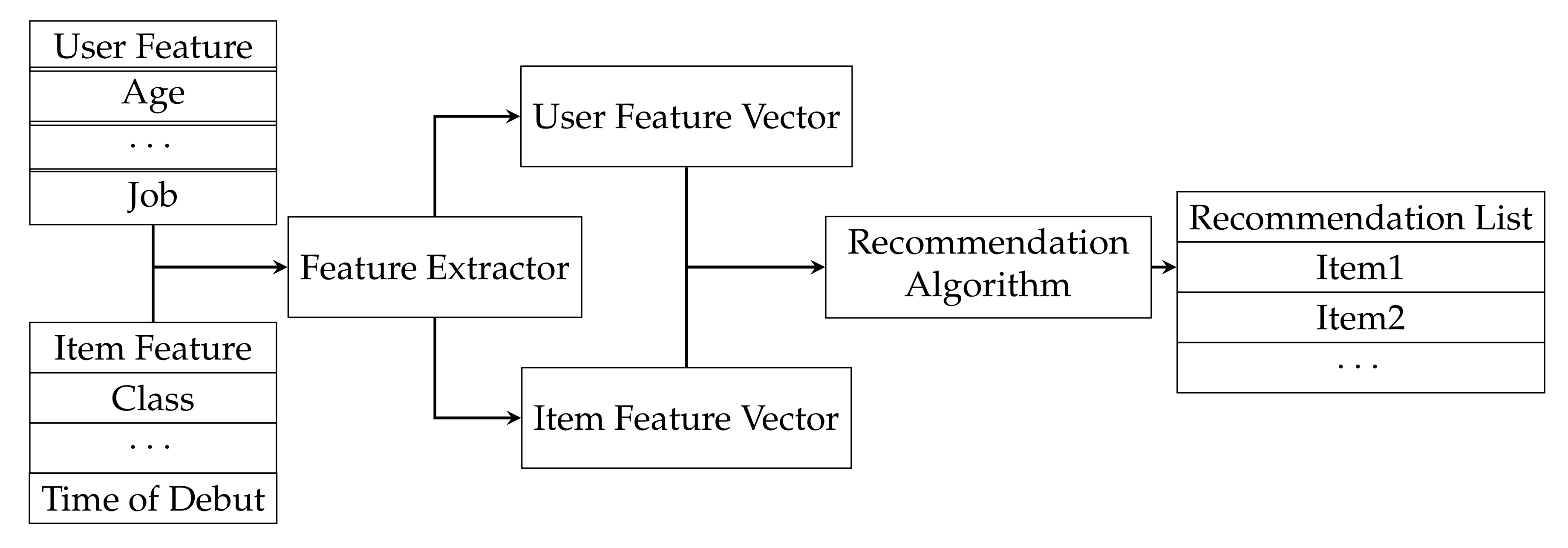
The standard procedure of the recommendation system can be seen in Figure 1. To begin with, we pre-train a set of user-item scores. Define $u_i$ to be the feature vector of user i, the value of which is in $\mathcal{U}\subset {\mathcal{R}}^{d_u}$; then, $v_j$ the feature vector of item j, the value of which is in $\mathcal{V}\subset {\mathcal{R}}^{d_v}$. The number of users is $\left|U\right|=N$, and the number of items is $\left|V\right|=M$. Denote the rating matrix as L. Therefore, we reach the fundamental objective, i.e., to calculate $p(U,V|L)$. Note that the matrix factorization way decomposes L to obtain $U,V$. 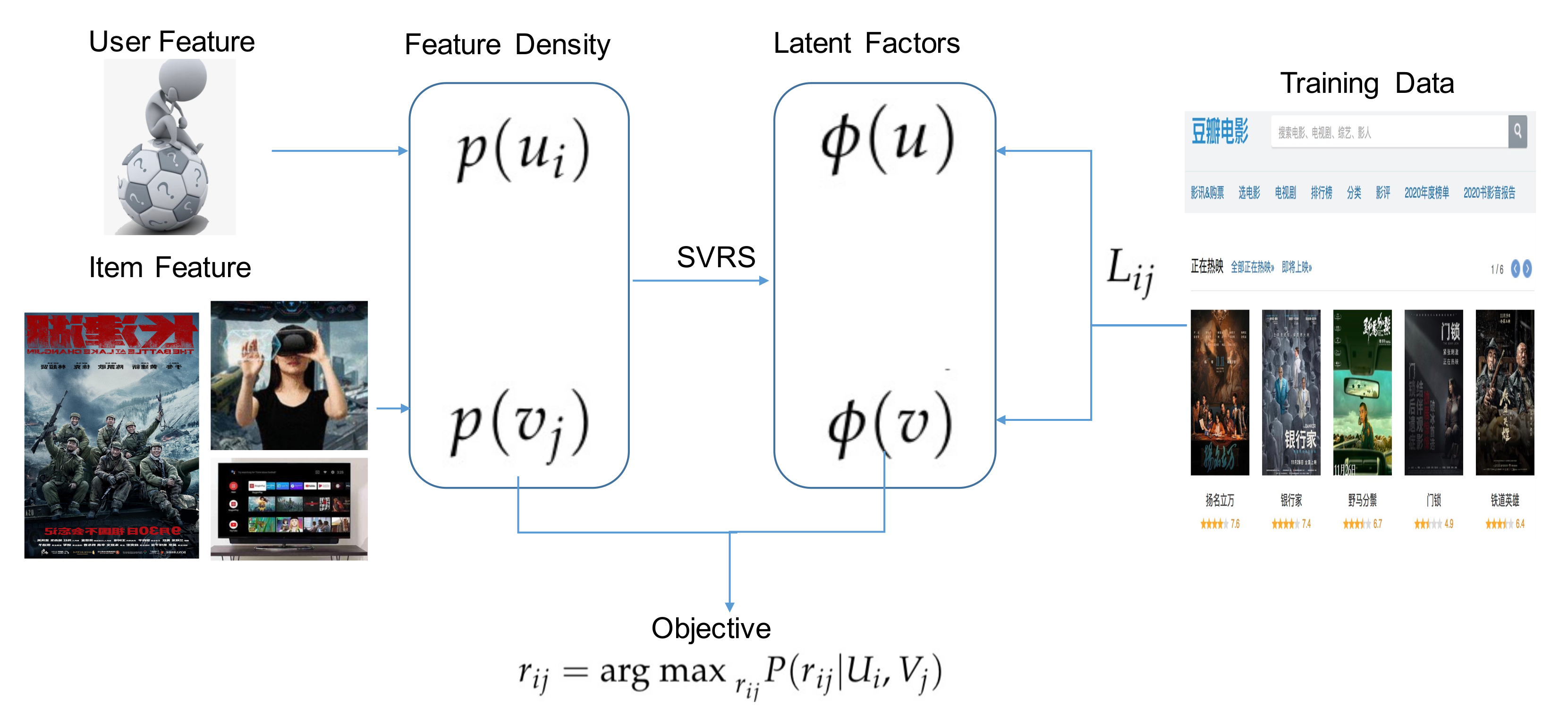After this, we use U and I, the ground truth of user and item feature, to further predict ratings that users have not given. Specifically, the objective of SVRS is to obtain the U and V that can maximize the likelihood, or minimize the Stein discrepancy. The user feature density is

$$\begin{array}{c}\hfill p\left(u\right):=\overline{p}\left(u\right)/Z,\end{array}$$

(7)

of which $\overline{p}\left(u\right):=p_0\left(u\right){\prod }_{i=1}^{N}p\left(L_i\right|u)$. $Z=\int \overline{p}\left(u\right)\mathrm{d}u$ is the normalization. Notice that U and V are calculated alternatively, and that, in order to save space, we may skip the derivation of V (see Figure 2 for the procedure of SVRS).

Figure 1. Procedure of the recommendation system.

Figure 2. Schematic of SVRS. (Training data is Douban Movie, left picture of Item Feature is blockbuster movie in China).

Traditionally, $p\left(u\right)$ is maximized by maximizing the function that has the same monotonicity with joint probability, a highly-demanding process to apply directly in VI. To calculate the log joint density, we can instead compute the evidence lower bound (ELBO), or the metrics that measure the difference (or distance) of $p\left(L\right|u)$ with $q\left(u\right)$—of which $q\left(u\right)$ is the approximate variational distribution [28]:

$$\begin{array}{cc}\hfill \log \left(p\right(L\left)\right)& =\int q(u)\log (p(L,u))\mathrm{d}L-\int q(u)\log (q(u))\mathrm{d}L+\hfill \\ & (-\int q(u)\log (\frac{p(L|u)}{q(u)})\mathrm{d}L)\hfill \\ \hfill & =\mathcal{L}(u)+\mathrm{KL}(q||p),\hfill \end{array}$$

(8)

where $\mathrm{KL}\left(q\right|\left|p\right)=-\int q\left(u\right)\log \left(\frac{p\left(L\right|u)}{q\left(u\right)}\right)\mathrm{d}L$, $q\left(u\right)={\prod }_{i=q}^N{q}_i\left(u_i\right)$.

Thus, two methods can be used to obtain the target distribution that can maximize the log likelihood of L, maximizing ELBO or minimizing $\mathrm{KL}\left(q\right|\left|p\right)$. We choose the second one. In order to minimize the KL divergence, we need to differentiate it with respect to $q\left(u\right)$. This is not easy. Thus, we have to set $q\left(u\right)$ to simple forms, or use MCMC sampling instead. In this work, we choose the first popular way.

SVRS requires some assumptions before we can proceed. To begin with, we assume the rating noise is Gaussian,

$$\begin{array}{cc}\hfill p\left(L_{ij}\right|U_i,V_j)& =\mathcal{N}(U_i{V}_j,{\delta }^2)\hfill \\ \hfill & =\log \frac{1}{\sqrt{2\pi }\delta }\exp (-\frac{L_{ij}-U_i{V}_j}{2{\delta }^2}).\hfill \end{array}$$

(9)

Since we use $q\left(u\right)$ and $q\left(v\right)$ to replace $p\left(L\right|u,v)$, we need to first define which form of $q\left(u\right)$/$q\left(v\right)$ is best-suited. Clearly, the optimal $q\left(u\right)$ and $q\left(v\right)$ have the smallest divergence with $p\left(L\right|u,v)$. Thus, the best $q\left(u\right)$ and $q\left(v\right)$ have the following form:

$$\begin{array}{cc}\hfill q^{*}\left(u\right)& =\arg {\min }_{q\in {\mathcal{Q}}_u}\mathrm{KL}\left(q\right|\left|p\right)\hfill \\ \hfill & ={\mathbb{E}}_q\left[\log q\left(u\right)\right]-{\mathbb{E}}_q\left[\log \overline{p}\left(u\right)\right]+const.,\hfill \end{array}$$

(10)

$$\begin{array}{cc}\hfill q^{*}\left(v\right)& =\arg {\min }_{q\in {\mathcal{Q}}_v}\mathrm{KL}\left(q\right|\left|p\right)\hfill \\ \hfill & ={\mathbb{E}}_q\left[\log q\left(v\right)\right]-{\mathbb{E}}_q\left[\log \overline{p}\left(v\right)\right]+const.,\hfill \end{array}$$

(11)

of which ${\mathcal{Q}}_u$ is $q\left(u\right)$’s space, and ${\mathcal{Q}}_v$ is $q\left(v\right)$’s space. Intuitively, the best $\mathcal{Q}$ possesses the feature of accuracy and tractability. Therefore, it is rational to choose linear $\mathcal{Q}$ that is continuous and differentiable (in another perspective described in other papers, this is the trick of reparameterization) [29].

In this way, using

$$T\left(u\right)=u+\rho \varphi \left(u\right),$$

(12)

we can simplify the computing and differentiating process. $\rho$ denotes the step-size, and $\varphi \left(u\right)$ is selected simple density. If we take Equation (12) as the updating function, then $\varphi \left(u\right)$ will be the updating direction. T can be viewed as a map that is invertible and monotone [30]. It is our goal to output data points to model the posterior distribution. Therefore, we initially produce some data points and then update $\varphi \left(u\right)$ instead gradually in order to obtain the final optimal data sets. Notice that there is always a measurable map T if q and p are atom-less density.

Based on Liu et al.’s work [25], there is a close connection between KL divergence and Stein’s identity, and we obtain the following conclusion:

Theorem 1.

Letting $T\left(u\right)=u+\rho \varphi \left(u\right)$ and $q_{\left[T\right]}=q_{\left[T\right]}\left(T\left(u\right)\right)$, one can obtain

$${▿}_{\rho }\mathrm{KL}(q_{\left[T\right]}{\left|\right|p\left)\right|}_{\rho =0}=-{\mathbb{E}}_{\mathbf{u}\sim q}\left[\mathrm{trace}\left({\mathcal{A}}_p\varphi \left(u\right)\right)\right],$$

(13)

where ${\mathcal{A}}_p\varphi \left(r\right)={▿}_r\log p\left(r\right)\varphi {\left(r\right)}^T+{▿}_r\varphi \left(r\right)$ is the Stein operator.

Proof. 

Seen from Equation (13) with (2), one can obtain $\varphi \left(u\right)$ that iteratively reduces the KL-divergence. □

Thus, we can obtain $\varphi \left(u\right)$ by solving the maximum of ${\mathbb{E}}_{\mathbf{u}\sim q}\left[\mathrm{trace}\left({\mathcal{A}}_p\varphi \left(u\right)\right)\right]$, which is computed according to Theorem 1.

Theorem 2.

The Stein’s variational direction is the steepest updating direction $\varphi \left(r\right)$ in an RKHS ${\mathcal{H}}^d$ with dimension d, which is:

$${\varphi }^{*}\left(u\right)={\mathbb{E}}_{\mathbf{R}\sim q}[{▿}_r\log p\left(r\right)\varphi {\left(r\right)}^T+{▿}_r\varphi \left(r\right)],$$

(14)

in which $\varphi {\left(u\right)}^T=k(u,·)$.

This indicates that the negative gradient direction of Equation (12) is also the derivative of the KL-divergence w.r.t. $p\left(u\right)$, which is also equal to $p\left(u\right)$’s Stein discrepancy.

Thus, we obtain the updating equation

$$q_{l+1}=q_{l\left[T_l^{*}\right]},$$

(15)

where $T_l^{*}\left(u\right)=u+{\rho }_l{\varphi }_{q_l,p}^{*}\left(u\right)$. In this way, we have converted the problem of calculating the user density $p\left(u\right)$ into a Stein VI optimization that calculates data points of $p\left(u\right)$. Thus, SVRS can be summed up in Algorithm 1.

Algorithm 1 SVRS.

Input ${\left\{U_0\right\}}_0^M,{\left\{V_0\right\}}_0^M,{\varphi }_i,{\varphi }_j,{\rho }_0,Z_{ij}$ Output: U,V,$r_{ij}$ for each label $Z_{ij}$ do  $U_i^{(t+1)}\leftarrow U_i^t+{\rho }_t{\widehat{\varphi }}_i^{*}$ where  ${\widehat{\varphi }}_i^{*}=\frac{1}{n}{\sum }_{i^{\prime }=1}[k(u_{i^{\prime }}^t,u){▿}_{u_{i^{\prime }}^t}\log p\left(u_{i^{\prime }}^t\right)+{▿}_{u_{i^{\prime }}^t}k(u_{i^{\prime }}^t,u)]$  $V_j^{(t+1)}\leftarrow V_j^t+{\rho }_t{\widehat{\varphi }}_j^{*}$ where  ${\widehat{\varphi }}_j^{*}=\frac{1}{n}{\sum }_{j^{\prime }=1}[k(v_{j^{\prime }}^t,v){▿}_{v_{j^{\prime }}^t}\log p\left(v_{j^{\prime }}^t\right)+{▿}_{v_{j^{\prime }}^t}k(v_{j^{\prime }}^t,v)]$ end for until convergence Output:$U_i,V_j,r_{ij}=\arg \max {}_{r_{ij}}P\left(r_{ij}\right|U_i,V_j)$ Compute: MAE, RMSE.

A detailed analysis of the appendix shows that SVRS is unbiased and converging, and that it is closely related to the popular PMF and CF models.

3.1. Convergence Proof

Defining the bounded Lipschitz metric as the maximum difference of their mean values on a continuous text function,

$$\begin{array}{cc}\hfill \mathrm{BL}(u,v)=& {\sup }_f\{{\mathbb{E}}_{u}f-{\mathbb{E}}_{v}fs.t.{\parallel f\parallel }_{BL}\le 1\}\hfill \\ \hfill & \mathrm{where}{\parallel f\parallel }_{BL}=\max \{{\parallel f\parallel }_{\infty },{\parallel f\parallel }_{Lip}\},\hfill \end{array}$$

(16)

where, according to Liu et al. [26], we have:

Theorem 3.

Assuming ${\mathcal{A}}_{p}k(u,u^{\prime })$ is bounded Lipschitz on $(u,u^{\prime })$ with a limited norm, then, for any two probability measures $s,t$, we have

$$\mathrm{BL}(T\left(u\right),T\left(u^{\prime }\right))\le (1+2\rho ){\parallel {\mathcal{A}}_{p}k(u,u^{\prime })\parallel }_{BL}\mathrm{BL}(u,u^{\prime }).$$

(17)

In addition, furthermore, we have:

Theorem 4.

Let $\widehat{p}{\left(u\right)}_t$ be the empirical measure of $U_t^i$ at the tth iteration of SVRS, and assume

$${\lim }_{M\to \infty }\mathrm{BL}(\widehat{p}{\left(u\right)}_0^M,p{\left(u\right)}_0^{\infty });$$

(18)

then, for $p{\left(u\right)}_t^{\infty }=T\left(p{\left(u\right)}_{t-1}^{\infty }\right)$, we have

$${\lim }_{M\to \infty }\mathrm{BL}(\widehat{p}{\left(u\right)}_t^M,p{\left(u\right)}_t^{\infty }).$$

(19)

This suggests that, as long as the initial data points converge, the final result’s probability measure will surely converge, which means that SVRS will introduce no further divergence during iteration. Furthermore, from the property of RKHS, and treating the data points obtained from each iteration, the density represented by the data points can be treated as a convergent sequence, which is unique for map T. Therefore, the theoretical final measure reached by a sequence of T is a fixed point. We therefore can show that SVRS has good convergence property.

Unbiasedness and Variance

Assuming that the final variational distribution we obtained is $q_{\theta }^{*}$, then the gradient of $q_{\theta }^{*}$ with respect to $\theta$ is ${\varphi }^{*}$. Since the SVRS algorithm produces a sequence of particles $\left\{U_i\right\}$ that construct the objective distribution $p\left(u\right)$ (and $p\left(v\right))$. We can say that $f\left(\left\{U_i\right\}\right)=p\left(u\right)$. If f is continuous at the value space of $\theta$, and $\left\{U_i\right\}$ is the unbiased samples of $q_{\theta }^{*}$, we can see that $f\left(\left\{U_i\right\}\right)$ is also the unbiased estimation of $p\left(u\right)$.

In addition, the Fisher information [31] of $\theta$ is ${\mathbb{E}}_{\theta }{\left[\frac{\partial \log q_{\theta }\left(u\right)}{\partial \theta }\right]}^2$. Since the updating direction of $\theta$ is also connected to the updating direction of $\varphi$, we can see that the Stein discrepancy is closely related to the Fisher divergence, which is $\mathbb{F}(q,p)={\mathbb{E}}_{x\sim q}\left[{\parallel s_p\left(x\right)-s_q\left(x\right)\parallel }_2^2\right]$. According to the Cramer–Rao bound, we have

$${\mathrm{Var}}_{\theta }\left(\delta \right)\ge \frac{{\left(T_{\theta }^{\prime }\right)}^2}{{\mathbb{E}}_{\theta }{\left[\frac{\partial \log q_{\theta }\left(u\right)}{\partial \theta }\right]}^2}.$$

(20)

Therefore, we have the lower variance bound for SVRS. The reason is that the second part of Equation (14) acts as a repulsive force to drive the particles away from the sink value, i.e., the mean value of the target distribution, causing the variance to increase. Interested readers can refer to Oates et al. [32] for variance reduction methods.

3.2. Connection with CF-Based Recommendation

SVRS can be treated as a kind of model-based CF algorithm. A typical model-based CF algorithm first develops a model of user ratings, and then uses the probability approach to compute the expected prediction of user ratings on other items. From the perspective of Equation (10), computing the expected prediction is an intermediate step in SVRS, and, in a general sense, SVRS can be called a CF-based recommendation algorithm. However, a traditional CF-based algorithm computes the similarity between users or items, and then recommends a list of items according to the similarities, and in this sense, CF is just a kind of classification or cluster algorithm that produces the feature distance between users and items, and cannot scale or deal with sparsity.

3.3. Connection with PMF Models

PMF is a popular recommendation algorithm that has slightly better performance than others. However, PMF is only a very primitive form of loss optimization framework. Its main computing technique is the same as VI, or SVRS, formulating the user/item feature parameter into a posterior inference problem, and then solving the optimum by setting the derivatives with respect to the target parameter to 0. The differences are that the PMF is not general, which requires a specific assumption of the prediction distribution, and it does not treat the recommendation problem as a general variational optimization framework.

4. Experiment

In this paper, we evaluate SVRS in terms of the most important measure for recommendations, MAE and RMSE. The data sets used are Movielen-1M, Movielens-10M and Douban datasets. In addition, the results are averaged. To compare more subjectively, we compare SVRS with MV, PMF, BPMF, AutoRec, NADE, DLTSR, DVMF and SVRS.

4.1. Configurations

Then, we introduce the experimental setting (Some of the settings can be seen in Table 2). The training data are a matrix with rating scores ranging from [1, 5]. Before comparing with DL-based recommendation algorithms, we first train those DNNs. When training with the MovieLens-100K as well as MovieLens-1M, use minipatches of 10,000 to speed up convergence. The regularization coefficient of PMF is $\lambda =0.001$, and the user feature dimension is 10. The regularization coefficient of BPMF is $\lambda =0.002$, and the user feature dimension is 30. With respect to AutoRec, we use a three layers neural network, and set $\lambda =1$. The number of neurons is 250 for MovieLens-100K and MovieLens-1M, 500 for Douban datasets. NADE has the same settings as Autorec, with 0.05 the learning rate. As another DL-based recommendation algorithm, DLTSR takes much training time, and needs to be accelerated. The reason is partly high at 0.01, and the regularization parameter is $\lambda =0.02$. For DVMF, we use five layers and set $\lambda =0.001$. The number of neurons is 750 for MovieLens-100K, 2400 for MovieLens-1M, 1600 for Douban datasets. As for SVRS, the user density and item density prior are assumed to be Gamma distribution. In addition, we repeat multiple times to obtain MAE and RMSE.

Table 2. Parameter setting.

Parameter	Commentary	Value
$p\left(u_i\right)$	feature of user i
$p\left(v_j\right)$	feature of IoT service j or item j
$\varphi \left(u\right)$	smooth vector functions used to approximate $p\left(u\right)$
$\varphi \left(v\right)$	the smooth vector functions used to approximate $p\left(v\right)$
$L_{ij}$	initial ratings
${\mathcal{A}}_p\varphi \left(u\right)$	the Stein operator,
$\mathcal{D}(q,p)$	Stein discrepancy
$\lambda$	regularization parameter	0.001, 0.002, 1

4.2. Convergence

We demonstrate the influence of sample number and step-size $\rho$ on SVRS in terms of testing accuracy and running time. It is easy to see from Figure 3a that a smaller step-size, i.e., [0.01, 0.05] leads to higher accuracy while a larger step-size contributes to fluctuating accuracy. However, due to the feature of scalability, SVRS maintains higher accuracy despite step-size changes. In addition, the change of step-size only affects SVRS running time. Of course, smaller step-size often leads to slower convergence, which is shown in Figure 3b. Furthermore, sample numbers (the number of data points produced by SVRS to approximate the posterior density) can also impact convergence rate. Therefore, in order to find the most efficient parameters, we have to select carefully to reach the optimal result. Therefore, we set $\rho =0.05$ and $M=100$.

Figure 3. Testing accuracy and running time under different M. (a) testing accuracy under different M; (b) running time under different M.

4.3. Analysis

Figure 4a shows the results using datasets MovieLens-100K and MovieLens-1M in terms of RMSE. It is easy to see that SVRS improves by 0.19% compared with the DVMF. Note that DLTSR reaches the same result as SVRS because it adapts to different training data and is computationally efficient. In summary, SVRS performs better than other algorithms.

Figure 4. RMSE and MAE Comparison. (a) comparison under MovieLens data; (b) comparison under Douban data; (c) comparison under MovieLens data; (d) comparison under Douban data.

Figure 4b shows the results using MovieLens-100K and MovieLens-1M in terms of MAE. It is easy to see that SVRS improves by 2.3% compared with the DVMF. Figure 4c shows the results using Douban data in terms of RMSE. It is easy to observe that SVRS improves by 0.15% compared with the DVMF. Figure 4d shows the results using Douban data in terms of MAE. It is easy to see that SVRS improves by 2.15% compared with the DVMF.

5. Discussion

We evaluate the performance in terms of convergence and accuracy using MovieLen and Douban datasets of the algorithm and the results reported in Section 4. In summary, (Stein Variational Recommendation) SVRS has the quality of good convergence, accuracy, and low complexity. As long as the initial data points converge, SVRS will not introduce further divergence Specifically, the convergence rate of SVRS is satisfactory. It depends on parameters such as step size, sample numbers, etc. The accuracy of SVRS is slightly higher than its existing counterparts.

SVRS also possesses unbiasedness and convergent variance, essential for convergence behavior and accuracy when the dataset scales. SVRS is also closely related to popular CF-based recommendations and PMF models in terms of the design process. This gives SVRS a promising future to be generalized. SVRS offers a powerful way to infer ground truth about users and items. However, the development of SVRS is still at its early age, and most existing works focus on theoretical analysis. We believe that, in the future, the true benefits of Stein Variational recommendation will be found in more applications by providing services for the Internet of Things.

6. Conclusions

Providing convenient and useful IoT services requires solving the problems facing the online recommendation systems. The target of this paper is to propose and verify a novel Stein variational inference based recommendation algorithm—SVRS that infers the ground truth density of latent variables and predicts the ratings of items they might give. Users who have not viewed a particular piece of content can also be predicted via this algorithm. We offer insights into how user ratings are formed in our SVRS, and we can extend its capabilities to incorporate more dimensions. SVRS performs better than existing algorithms by simulations.

In the future, we will try to apply SVRS to more applications to solve the most prominent problems in the industry and continue to study the most accurate and practical ground truth analysis methods. Specifically, there are four promising areas that can be explored. The first is how to identify the factors or parameters that can influence the performances of SVRS. In the current literature, most authors compare their models’ best performance with others to verify them. However, any model’s performance is not fixed, all subject to the change of settings, data quality, model dimension and model complexity. It is urgent to build a unified platform that can show readers and researchers the advantages and disadvantages of SVRS for their information. The second is how to build SVRS based recommendation models that can adapt to complex network structures. In the existing literature, most Stein variational recommendation-based models use a different simplification method to deal with networks with complex structures. Therefore, it is necessary to develop recommendation models that require less simplification and adapt to complex models. The third is how to unify SVRS with different kinds of recommendation models. As we have seen in the above discussions, SVRS has a close relationship with other recommendation models, such as CF and PMF. There is no doubt that all those methods share some common methodology inherently. However, how to unify them together, or if they have differences that cannot be reconciled, the exact differences between them remain unexplored in the literature. The last is how to apply SVRS in the fields where there is no satisfying solution for recommendation or prediction. Since SVRS is a rather new tool in the literature, many fields lack the application of the Stein Variational-based method to solve the most prominent problems. Therefore, the wide application of the Stein variational recommendation-based method can not only promote the theoretical understanding of itself but also contribute to the research of other fields.