Experimental Investigation and Validation on Suppressing the Unsteady Aerodynamic Force and Flow Structure of Single Box Girder by Trailing Edge Jets

Abstract

In the present investigation, a wind tunnel experiment was performed to evaluate the effectiveness of the trailing edge jets control scheme to mitigate the unsteady aerodynamic force and flow structure of a single box girder (SBG) model. The flow control scheme uses four isolated circular holes for forming the jet flow to modify the periodic vortex shedding behind the SBG model and then alleviate the fluctuation of the aerodynamic force acting on the test model. The Reynolds number is calculated as 2.08 × 10⁴ based on the incoming velocity and the height of the test model. A digital pressure measurement system was utilized to obtain and record the surface pressure that was distributed around the SBG model. The surface pressure results show that the fluctuating amplitude of the aerodynamic forces was attenuated in the controlled case at a specific range of the non-dimensional jet momentum coefficient. The Strouhal number of the controlled case also deviates from that of the original SBG model. Except for the pressure measurement experiment, a high-resolution digital particle image velocimetry system was applied to investigate the detailed flow structure behind the SBG model to uncover the unsteady vortex motion process from the SBG model with and without the trailing edge jets flow control. As the jet flow blows into the wake, the alternating vortex shedding mode is switched into a symmetrical shedding mode and the width of the wake flow is narrowed. The proper orthogonal decomposition was used to identify the energy of the different modes and obtain its corresponding flow structures. Moreover, the linear stability analysis of the flow field behind the SBG model shows that the scheme of trailing edge jets can dramatically suppress the area of unsteady flow.

1. Introduction

With the span of bridges increasing, the main girder of the bridge will become more flexible with lower stiffness and damping to resist the dynamic load. The wind load is the most common dynamic force acting on the long-span bridge in the natural environment [1,2]. Airflow flows across the bridge girder and yields the alternating vortex shedding in the wake. When the vortex shedding frequency is closed or equaled to that of the structure, the structure has the potential for the resonance phenomenon to occur, i.e., vortex-induced vibration (VIV). The VIV is the primary issue that is caused by airflow in bridge engineering because it occurs at a low velocity (e.g., the VIV of the Great Belt East Bridge was observed at an incoming flow velocity of 4–12 m/s as presented by Larsen et al. [1] and leads to structural fatigue when undergoing frequent vibration [3,4]. Therefore, it is necessary to present an efficient control scheme to suppress the amplitude of VIV [4,5,6,7].

The external shape of the bluff body can influence the performance of the VIV [8]. If the target structure is streamlined, the flow separation cannot occur and the alternating vortex shedding cannot form; it is hard for the VIV to appear in those structures. Therefore, the box girder of the bridge is designed as near streamline for alleviating the VIV. Due to the box girder being not entirely streamlined, the VIV often happens when the airflow velocity attains a specific value, i.e., the wake vortex frequency is equal to that of the box girder at this velocity [2,9]. In addition, the affiliate parts (i.e., railing, maintenance track, and streetlamps) that are set in the box girder also can affect the characteristics of the main girder and the fluctuation of the aerodynamic force. Zhan et al. [10] changed the straight railing along the span-wise direction to the wave railing for forming the three-dimensional disturbance to mitigate the VIV of a long-span bridge. The results indicated that when the wave length of the wavy bar was set as 0.5 or 1 times of the bridge girder height, the vertical and torsional VIV amplitudes were entirely suppressed and both sides of the upper surface were the best installation locations. However, this form of wave railing will occupy more space, impacting usability. The size and location of the horizontal bar of the railing had a dramatic influence on the flow structure of the position near the leading edge and the torsional VIV responses of the main girder as presented by Nagao et al. [11]. Moreover, Xin et al. [12] studied the effect of the inclination angle of the railing on the VIV of the bridge girder. For suppressing the VIV, the control effectiveness of the inclined railing was superior to the railing with the inclination angle of zero.

In addition to using non-structural parts to suppress the wind-induced vibration, many other control strategies, such as the structural and aerodynamic measures, have been presented in recent years [7,13,14,15]. Larsen et al. [7] designed tuned mass dampers (TMDs) to mitigate the vibration amplitude of the Great Belt East bridge. The results found that the VIV response of the bridge girder with TMDs was at the allowed range using a time-domain simulation. Battista and Pfeil [13] applied the TMDs in the Rio-Niterói Bridge to alleviate the VIV amplitude. They discovered that subsidiary active or tuned vibration absorbers had a remarkable influence on attenuating the dynamic responses on the main girder. Dai et al. [16] studied the parameter determination of the tuned mass damper in alleviating the VIV of the bridge girder. They found that the equivalent damping ratio (EDR) is only determined by the TMD parameters, not the aerodynamic parameters. Moreover, the EDR is closely related to the uncertainty in the stiffness of the bridge according to the result of the uncertainty analysis. The underlying control mechanism of TMD is that changing the vibrational frequency and the structural damping mismatch the frequency of the aerodynamic force. Due to the fluctuation of aerodynamic force or vortex shedding being mainly wind-induced oscillation, El-Gammal et al. [17] used a span-wise sinusoidal perturbation set on the two sides of a plate girder to disturb the span-wise vortex shedding and reduce the dynamic response of VIV. The results indicate that the vibration amplitude was reduced with a higher wave steepness in the span-wise sinusoidal perturbation. Larsen et al. [1] utilized a guide vane that was equipped in the lower sides of the Great Belt East Bridge to alleviate the airflow separation. This investigation indicated that the guide vane could suppress the alternating vortex shedding and mitigate the VIV responses. However, this method possesses slight control effectiveness at a low Re because less airflow goes through the guide vane to form the jet flow. The technique of leading-edge and trailing edge holes and the communicating channel formed the self-suction-and-jet (SSJ) flow as designed by Chen et al. [18]. These experimental results showed a reduction of the unsteady surface pressure and aerodynamic force, and the near-wake flow structure was steadier. In addition, the unsteady flow was shifted further downstream by using the control method of SSJ flow. To avoid the strength limit of the suction or jet flow, the control scheme of active suction or jet flow is presented. Zhang et al. [19] adopted active suction holes that were distributed on the bottom surface of the box girder with a specific interval to produce a Mode A secondary unstable wake flow, which can deeply alleviate the fluctuating amplitude of the aerodynamic force that is acting on the bridge girder. Chen et al. [20] designed an active control strategy with a leading-edge suction and trailing edge jet (LSTJ) that were inserted in the box girder to control the unsteady flow structure and aerodynamic force. They found that the best control case alleviated the unsteady lift force by about 37.88% and shrank the unsteady wake flow area by about 69.90%.

Inspired by the investigation result of Chen et al. [20], we only set the jet holes in the trailing edge of a single box girder (SBG) model to control the unsteady surface pressure, aerodynamic force, and unsteady flow structure. The present study is to investigate the control ability of the trailing edge jet for alleviating the unsteady aerodynamic force and the flow field of a single box girder and study what can influence the local separation on the upper and lower surface near to the leading edge of the SBG model. Only the trailing edge jet can reduce the energy consumption compared with the LSTJ as presented by Chen et al. [20]. The analysis methods of proper orthogonal decomposition (POD) and linear stability analysis were used to reveal the underlying control mechanisms of the trailing edge jets. The structure of the present paper is arranged as follows. The experimental setup, test model details with and without the trailing edge jets are given in Section 2. The analysis results of the surface pressure distribution, aerodynamic force, flow structure, POD modes, and linear stability analysis are presented in Section 3. The conclusions are given in the last section.

2. Experimental Setup and Details

The present investigation was performed in a closed-circuit wind tunnel (SMC-WT1) belonging to the Joint Laboratory of Wind Tunnel and Wave Flume, Harbin Institute of Technology, P. R. China. The closed-loop wind tunnel test section, which has a geometric scale of 505 $\times$ 505 mm² in cross-section and 1050 mm in the airflow direction, possesses optically transparent walls to observe the experimental phenomenon conveniently. The honeycombs, mesh structure, and contraction section were installed upstream of the test channel to produce a high-quality uniform incoming flow entering the square test channel. The incoming flow velocity can be successively regulated at the range of 0–25 m/s. The turbulence intensity level of the free incoming flow was evaluated as less than 0.4%.

2.1. Original Test Model Details

Figure 1 displays the sketch of the SBG model that was used in the current investigation. The Great Belt East Bridge, whose geometric scale of the main girder is 31 m in width and 4.34 m in height, possesses a main span of 1624 m. The SBG model was derived from the Great Belt East Bridge (Denmark) due to this bridge frequently occurring VIV at low airflow speed [1,20]. The SBG model was produced using a high-precision three-dimensional printer with a scale ratio of 1:125. Therefore, the SBG model had a width (B) of 248 mm, a height (H) of 34.72 mm, and a length (L) of 480 mm in the span-wise direction, as shown in Figure 1a,c. The slope surface on the carriageway was considered. The secondary structures on the surface of the bridge girder were neglected in this investigation. The Reynolds number was calculated as Re = 2.08 × 10⁴ according to the incoming flow velocity of 9 m/s and the height of the SBG model. It should be declared that despite the Re of the present experiment being much less than that of the real bridge in a natural wind environment, this investigation aimed to study the control effectiveness of the control scheme of the trailing edge jets. There were two iron bars that were used to firmly fix the SBG model in the test channel to prevent displacement and vibration during the experiment. The coordinate system was set as shown in Figure 1a. The positive X and Y are defined as the airflow and upward directions, respectively. The positive Z meets the right-hand rule.

2.2. Test Model with the Trailing Edge Jets

To realize the trailing edge jet flow, four isolated circular jet holes were uniformly spaced in the trailing edge of the SBG model. The space between two neighboring jet-holes was set as 100 mm (~2.88 H), and the diameter of each jet-hole was 6 mm (~0.17H), as shown in Figure 1 a,b. The center of the section of all the jet holes was situated at the cusp of the trailing edge of the SBG model. Polyvinyl chloride (PVC) tubes were used to connect the jet holes with the air accelerators. To allow for real-time control, the velocity of the jet flow of the jet-holes, the mass, and the volumetric flow controllers (FMA-2621A, measuring range: 0–1500 SLM) were utilized to set and monitor the airflow rate in the PVC tubes. A total of nine volumetric flow rates (Q_j) were conducted in the experimental investigation, as shown in

Table 1. J_sj for the SBG model with different jet rates.

Volumetric Flow Rate Qj (m3/h)	Jet Velocity Uj (m * s−1)	Non-Dimensional Jet Momentum Coefficients Jsj
0 (Original main girder model)	0	0
1.80	4.42	0.0016
2.88	7.07	0.0042
3.60	8.84	0.0066
4.32	10.61	0.0094
5.40	13.26	0.0147
7.20	17.68	0.0262
9.00	22.10	0.0409
10.80	26.53	0.0590
12.60	30.95	0.0802

. Based on the flow rates and the area of the jet-hole, the average velocity jet out from the jet-hole was obtained. In the present study, the non-dimensional jet momentum coefficient (J_sj) was applied to evaluate the strength of the jet flow blowing out from the jet-hole of different controlled cases [18,20,21,22], which could be defined as Equation (1).

$$J_{sj}=\frac{U_j{}^2{A}_h}{U_0{}^{2}HL}$$

(1)

where $U_j$ and $U_0$ are the velocity of the jet flow and incoming flow, respectively; $A_h$ is the total area of all the jet holes. The J_sj of the SBG model with various jet speeds was calculated and displayed in Table 1.

2.3. Measurement Apparatus

The pressure that was distributed on the surface of the SBG model was obtained and recorded by a digital pressure scanner (MPS4264) that possessed 64 pressure measurement ports and a maximum acquiring frequency of 850 Hz. The pressure taps that were distributed around the test model were connected to the pressure scanner by the PVC tube with a length of 0.5 m and a radii of 0.45 mm. Based on the research findings of [23], the distortion effects that were caused by the tubing system that were used for the pressure measurements can be neglectable. All the pressure taps were set in one cross-section located in the middle of the SBG model, which is the same with plane II as given in Figure 1). Both the upper and lower surface of the SBG model had 23 pressure taps, as given in Figure 2. The acquiring frequency and recording time were set as 0.4 kHz and 60 s, respectively, in the present experiment. According to the scale of the SBG model and test channel of SMC-WT1, The blockage ratio was obtained as 6.67%. Therefore, the surface measurement results should be corrected by using the algorithm about the solid blockage and wake blockage presented by [24].

To visualize the characteristics of the wake flow structure behind the SBG model with and without the trailing edge jets, a high-resolution particle image velocimetry (PIV) system was used to record the photos of the target flow field. The sketch of the PIV experimental setup in the present measurement is given in Figure 3. The PIV system mainly contains three parts: illuminating, camera, and synchronizer. A high-speed double-pulse Nd: YAG laser (Vlite-Hi 200, Beamtech Optronics Corporation, Beijing, China), which has the highest work frequency of 200 Hz and energy of 100 mJ per pulse, was selected as the illuminating system to light up the target plane. The cylindrical lenses manipulated the laser beam to form a laser sheet with a thickness of about 1.0 mm in the measurement plane. A high-speed CCD camera (PCO: pco. dimax HS4, Kelheim, Germany) was applied to capture and save the photos of the measurement objectives, which possessed 2277-fps at the full-frame of 2000 × 2000 pixels. Moreover, we used a smoke generator that produced oil-droplets with a diameter of about 5 μm that were seeded into the airflow. The oil-droplets was served as the tracer particle whose movement could represent the airflow motion [25].

This investigation measured two vertical target planes, as given in Figure 1a. Planes I and II, the vertical target plane, were situated at the central section of the jet-hole and SBG model, respectively. The position of a CCD camera should be strictly perpendicular to the target plane during the experiment, as displayed in Figure 3. A total of 4000 pairs of photos were acquired at the trigger frequency of 200 Hz in every target plane of different experimental cases. The pixel of photos at the target plane I and II was 2000 × 1600 pixels² and 2000 × 1600 pixels², respectively. After obtaining the flow field photos, the cross-correlation operation was performed to extract the instantaneous velocity by adopting the interrogation window of 32 × 32 pixels and an efficient overlap rate of 50%. As a result, the spatial resolution of the instantaneous velocity in the measurement planes I and II were calculated as 1.8 × 1.8 mm² and 2.2 × 2.2 mm², respectively. It should be noted that the measurement uncertainty for the instantaneous velocity of the PIV measurement result was evaluated to be under 5%.

3. Experimental Results and Discussions

3.1. Surface Pressure Distribution

The pressure coefficient ($C_{pi}(t)$) was that the surface pressure results that were acquired by the pressure measurement experiment were nondimensionalized by the dynamic pressure and defined as Equation (2). The mean value of the external surface pressure coefficient ($C_p\_M$) was defined as Equation (3) to illustrate its average features. We used the standard deviation of the external surface pressure coefficient ($C_p\_R$) to describe the fluctuating characters of the pressure distribution, as given in Equation (4).

$$C_{pi}(t)=\frac{2(p_i-p_{\infty })}{\rho U_0{}_{}^2}$$

(2)

$$C_p\_M=\frac{1}{N}{\displaystyle \sum _{i=1}^N{C}_{pi}(t)}$$

(3)

$$C_p\_R=\sqrt{\frac{1}{N}{\displaystyle \sum _{i=1}^N{(C_{pi}(t)-\overline{C_{pi}(t)})}^2}}$$

(4)

where $p_i$ is the static pressure that is acting on the surface SBG model and $p_{\infty }$ is the static pressure of the free stream. The time histories of $p_i$ and $p_{\infty }$ are acquired and recorded by the digital pressure scanner. $\rho$ is the air density and N is the length of the total sample.

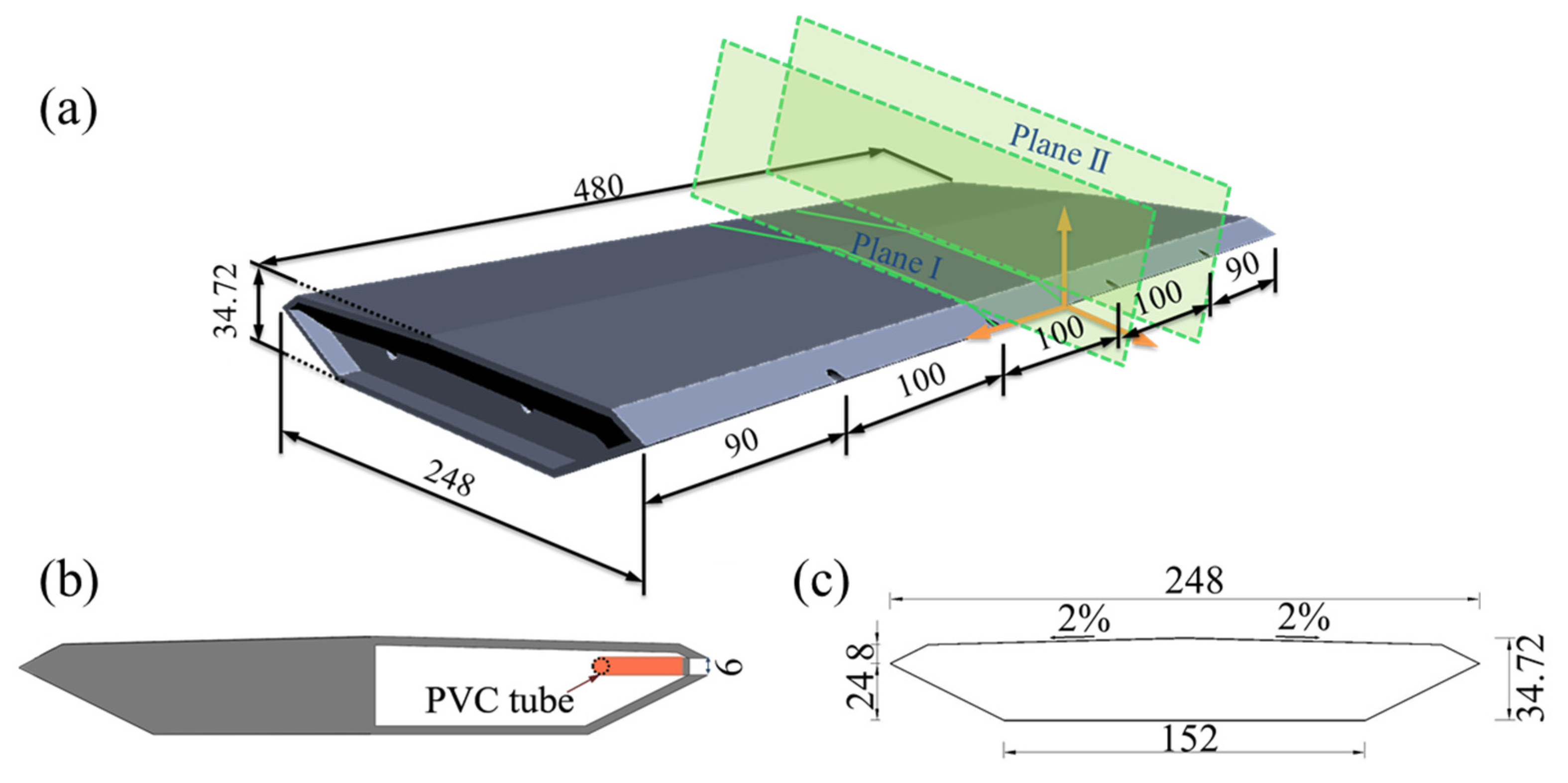
It should be illustrated that the surface pressure measurement plane was located in the central cross-section (i.e., plane II as given in Figure 1a) was far away from the jet holes. The pressure distribution on other cross-sections may be different. However, the aerodynamic force that was acting on the present cross-section of the controlled case might underestimate the control ability due to the pressure measurement section being the farthest distance from the cross-section with trailing jet hole [26]. The PIV result will confirm that. Figure 4 gives the external surface pressure coefficient that was distributed around the SBG model that was equipped with and without trailing edge jets.

For the case J_sj = 0, the mean pressure result of the upper surface on the SBG model shows a dramatic decrease due to an inflection point that existed between the pressure measurement taps 1 and 2. The adverse pressure gradient was observed at the range of X/B from 0.11 to 0.20, as shown in Figure 4a. Therefore, the flow separation occurs in that position, causing the fluctuating pressure to have a maximal value at X/B = 0.11, as shown in Figure 4c. As the X/B was larger than 0.20, the mean pressure distribution of the upper surface had similar values, except for the position of X/B = 0.5 and near the trailing edge. The upper external surface pressure distribution fluctuation shows an enormous value when X/B gets close to 1. The reason for this is that the position nearing the trailing edge will be more influenced by the alternating vortex shedding [20,26]. The adverse pressure gradient also appears in the lower surface of the SBG model at the position of X/B = 0.31–0.41 as shown in Figure 4b, and the peak value of the fluctuating pressure coefficient was obtained at the position of X/B = 0.31, as given in Figure 4d. Therefore, the local flow separation also occurred at the corner point between the pressure measurement taps 29 and 30. The other characteristics of the lower surface pressure are similar to those of the upper surface pressure.

When the jet holes were inserted in the SBG model, the external surface pressure was modified compared to that of the case J_sj = 0. The mean values of the external surface pressure of the controlled case with different non-dimensional jet momentum coefficients remain close to the uncontrolled case at the position nearing the leading edge of the SBG model. When the pressure taps were located at the trailing edge, the mean value of the external surface pressure was alleviated by the trailing edge jet flow, and the case J_sj = 0.0094 exhibited the best control effect. All the controlled cases can slightly attenuate the local flow separation at X/B = 0.11 of the upper surface of the SBG model, as shown in Figure 4c, compared to case J_sj = 0. However, the local flow separation was improved in the lower external surface of the controlled cases that caused a more considerable fluctuation of the pressure at X/B = 0.31, as given in Figure 4d. The fluctuation of the surface pressure close to the trailing edge was mitigated on both the upper and bottom surfaces of the SBG model with the trailing edge jets. That is because the jet flow can interrupt the alternating vortex shedding and lead to the wake flow being more steady. According to the pressure measurement results, the case J_sj = 0.0094 exhibited the best control ability for alleviating the mean value and fluctuation of the surface pressure. Obtaining better control effectiveness does not need larger non-dimensional jet momentum coefficients. There is an optimal non-dimensional jet momentum coefficient to realize the control effect, which is consistent with the study by Chen et al. [20] and Gao et al. [27].

3.2. Aerodynamic Force

The aerodynamic force can be obtained by integrating the surface pressure distributed around the SBG model. Afterward, the lift coefficient ($C_l(t)$), drag coefficient ($C_d(t)$), and the moment coefficient ($C_m(t)$) are calculated by Equation (5).

$$C_l(t)=\frac{F_l(t)}{\frac{1}{2}\rho U_0{}^{2}B},C_d(t)=\frac{F_d(t)}{\frac{1}{2}\rho U_0{}^{2}B},C_m(t)=\frac{F_m(t)}{\frac{1}{2}\rho U_0{}^2{B}^2}$$

(5)

where $F_l(t)$, $F_d(t)$, and $F_m(t)$ are the time-variant of the lift, drag, and moment force, respectively.

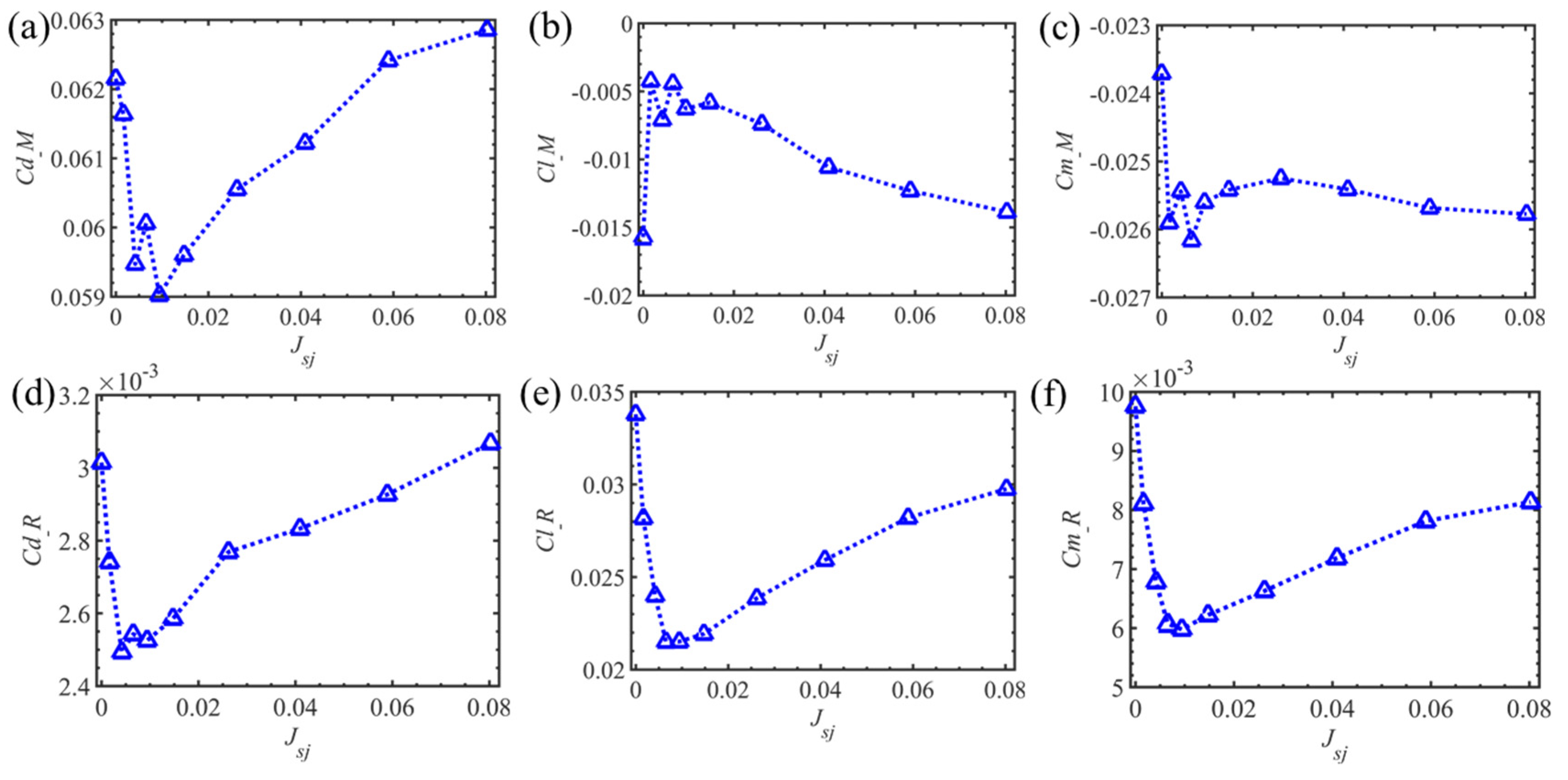
The aerodynamic coefficients that are acting on the SBG model that are equipped with and without control are displayed in Figure 5. The mean value of the drag coefficient of the case where J_sj = 0, which was consistent with the experimental results of 0.064 that were presented by Taylor et al. [28], 0.061 by Zhang et al. [9], and the numerical simulating result of 0.060 given by Frandsen [29], was obtained as 0.062. With the increase of the J_sj, both the mean value of the drag and lift coefficient shows a decrease at first and then an increase. However, the mean value of the moment coefficient of the controlled case maintained a closing value that was slightly large than the case where J_sj = 0, indicating that the different J_sj can not influence the moment force that is acting on the SBG model. Note that the main reason for the wind-induced vibration on the main girder is a large fluctuation of the aerodynamic force. The results of the fluctuation of the drag, lift, and moment coefficients that are acting on the SGB model with different J_sj are displayed in Figure 5d–f, respectively. The fluctuation of the aerodynamic coefficients were descending at first and then ascending with the increasing of J_sj. Therefore, an optimal J_sj for alleviating the unsteady aerodynamic force that is being exerted in the SBG model is required. This saturation phenomenon was also found by Chen et al. [20], Gao et al. [27], and Apelt et al. [30]. When the J_sj equals 0.0094, the best control ability was possessed in the present investigation. The control effect for the drag, lift, and moment coefficient fluctuation was 16.23%, 36.34%, and 38.74%, respectively. That conclusion agreed well with the results of the surface pressure analysis.

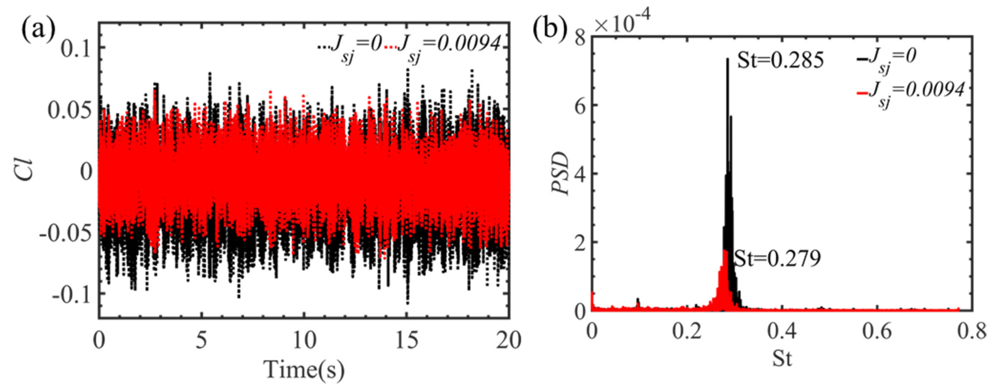
Figure 6 gives the time series and the power spectral density analysis of the lift coefficient being exerted in the SBG models with and without the trailing edge jets. The lift coefficient when J_sj = 0 shows a significant fluctuation during the experiment, as shown in Figure 6a. When the trailing edge jets were conducted in the SBG model with J_sj = 0.0094, the fluctuation of the lift coefficient was reduced compared to the case J_sj = 0. The peak value of the reduced frequency for the case J_sj = 0 was obtained to be 0.285 based on the fast Fourier transform (FFT) analysis, which was similar to that of 0.28 that was presented by Taylor et al. [28] and Chen et al. [18]. The amplitude of power spectral density analysis of the case J_sj = 0.0094 was lower than that of the case J_sj = 0, and the peak value of reduced frequency of the lift force was also changed to 0.279, given in Figure 6b. This indicates that the trailing edge jets that were equipped in the SBG model can modify the frequency and the strength of the vortex shedding behind the test model.

3.3. PIV Measurement Results

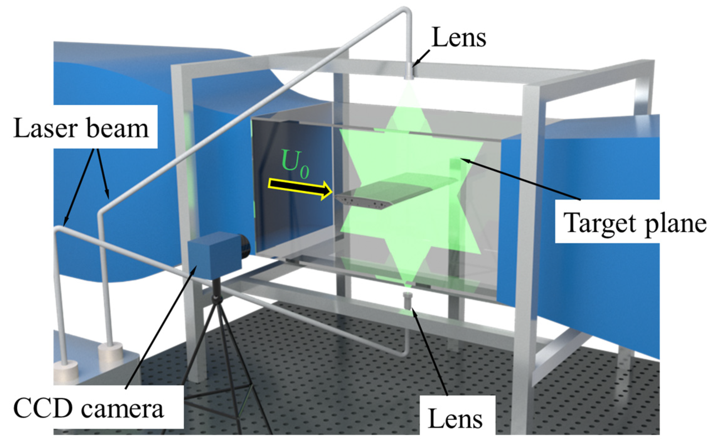
Besides the surface pressure measurement results, the PIV measurement experimental result can assist us in understanding the control mechanism of the trailing edge jets set in the SBG model.

Turbulence kinetic energy (TKE), which serves as a criterion to estimate the unsteady surface pressure and the fluctuating aerodynamic force that is acting on the SBG model [31,32,33], is calculated as follows:

$$\mathrm{TKE}=\frac{\overline{{u^{\prime }}^2}+\overline{{v^{\prime }}^2}}{2U_0^2}$$

(6)

where $u^{\prime }$ and $v^{\prime }$ are the fluctuating velocity components of the streamwise and transverse direction, respectively.

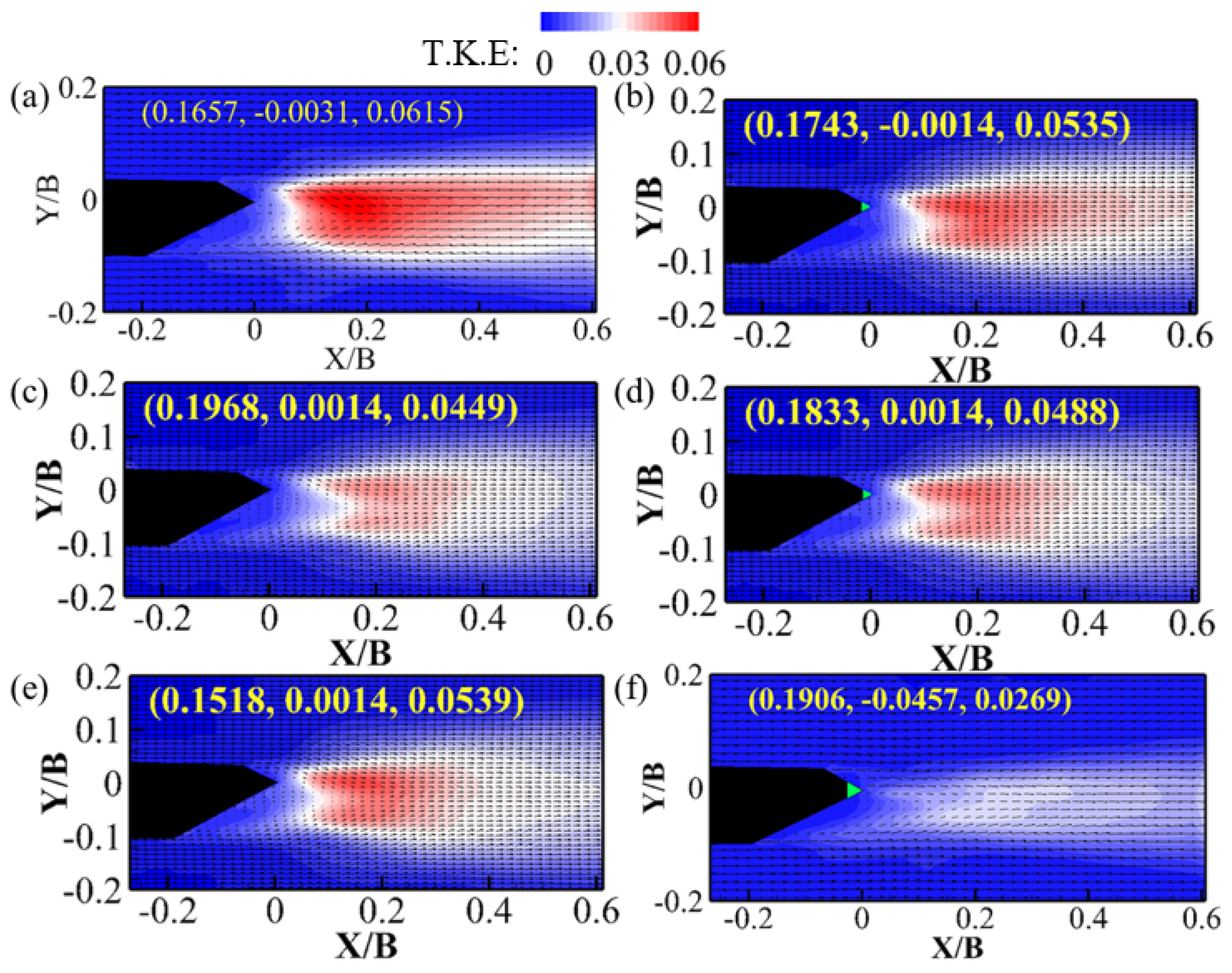
The time-averaged flow fields behind the SBG model in the two target planes with and without the trailing edge jets are given in Figure 7. A cluster of large values of the TKE is concentrated in the wake flow when J_sj = 0, as shown in Figure 7a. The reason is that the separation flows from the upper and bottom surfaces interact in the wake, leading to the velocity vectors colliding in this region. Therefore, the surface pressure distribution nearing the trailing edge when J_sj = 0 shows a dramatic fluctuation. As the trailing edge jets is conducted in the SBG model, the distribution area and maximum value of the TKE are reduced. Moreover, the maximum value of the TKE decreases at first and then increases with the enhancement of J_sj, as shown in Figure 7a–e, which can explain the changing trend of the fluctuation of the aerodynamic force that is being exerted in the SBG model. Compared to results from the target plane II, both the maximum value and the concentrated area of TKE in the target plane I of the case J_sj = 0.0094 is reduced as shown in Figure 7c,f. The unsteady aerodynamic force being exerted in the cross-section of plane I is lower than that of plane II, indicating the pressure measurement result that was obtained by plane II would underestimate the control effectiveness of a fluctuating value of surface pressure that is distributed on the SBG model with trailing edge jets. Moreover, the lower TKE value illustrates that the level of turbulence mixing in the wake flow of the controlled cases is lower than the uncontrolled case [34].

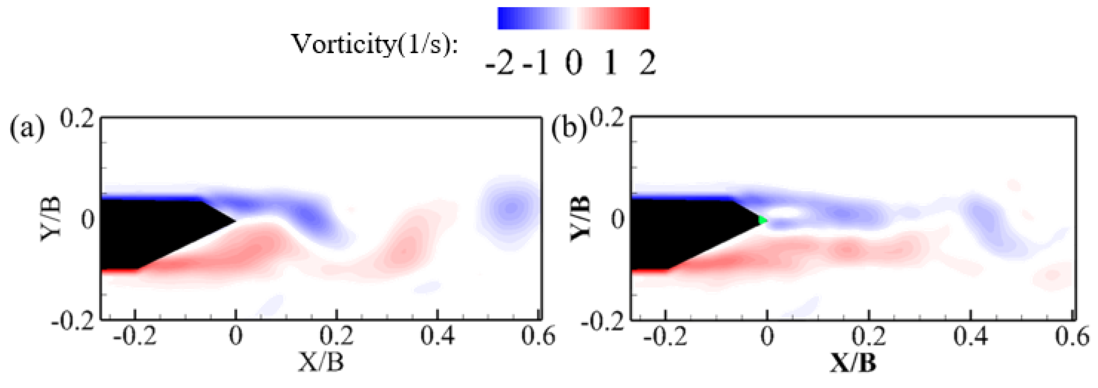
The instantaneous flow field in plane I that is given in Figure 8 illustrates the vortex shedding pattern behind the SBG model. A pair of asymmetric vortices alternating shed from the upper and bottom surface of the SBG model and a Karman vortex street can be obtained in the wake flow, which causes the significant fluctuation of the surface pressure on the trailing edge of the test model without control, as shown in Figure 4. The position where the upper and lower vortices interact leads to the enormous TKE value, which can be seen when comparing Figure 7a and Figure 8a. However, when the trailing edge jets work, a pair of symmetric vortices are formed in the wake flow field and the Karman vortex street is alleviated. The length of the vortex shedding is elongated and shifted further downstream, as given in Figure 8b. In addition, the jet flow interacts with the upper vortex and divides that vortex into some small-scale vortices, illustrating that the unsteady aerodynamic force that is being exerted in the SBG model is mitigated, and then the potential vortex-induced vibration can be prevented with the trailing edge jets [26].

At first, the proper orthogonal decomposition (POD) method was presented in the region of fluid mechanics by Lumley [35]. The snapshot POD that was introduced by Sirovich [36] was utilized in the present investigation. Here, every instantaneous photo that was obtained by the PIV experiment served as a snapshot of the flow structure. The autocovariance matrix was accepted by the product of the matrix of fluctuating part of the two-dimensional velocity and its transpose. The eigenvalues and the eigenvectors of the autocovariance matrix can be obtained. Afterwards, the accumulative energy proportion of each POD mode can be calculated by the eigenvalues of the autocovariance matrix, and the POD modes can be constructed from the basis built up from the snapshots.

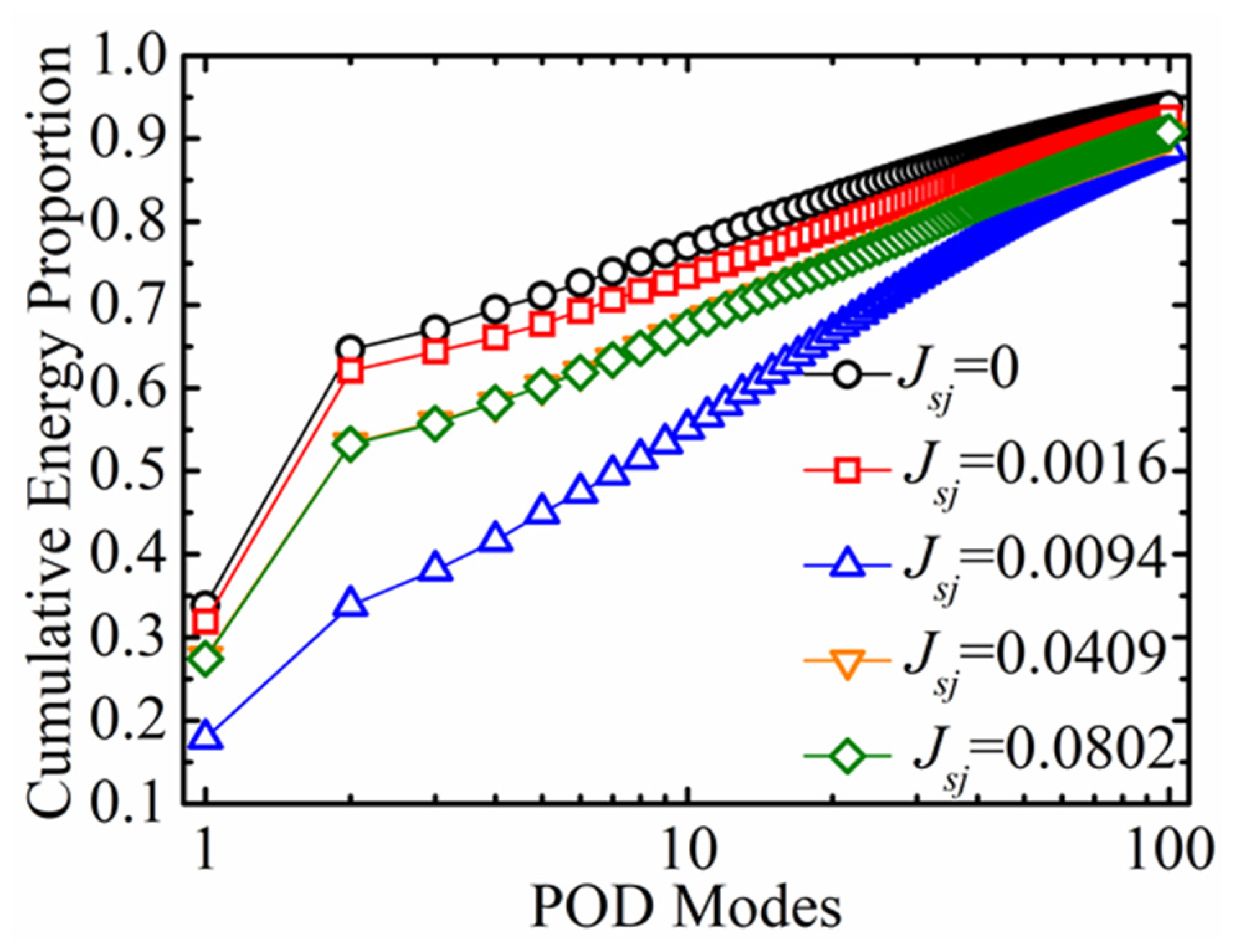
Figure 9 shows the percentage of the accumulative contribution of every POD mode to the total turbulence kinetic energy of the flow field for the different test cases in PIV measurement. It is observed that the first two POD modes possess 64.6% of the total energy for the case J_sj = 0. The first two POD modes represent the large-scale coherent structure, and the high-order POD modes represent the small-scale coherent structure as given by Feng et al. [37]. Therefore, the large-scale coherent structure plays an important role in the wake flow behind case J_sj = 0. When the control method is applied in the SBG model, the energy of each POD mode that is exhibited immensely changes. The total energy of the first two POD modes is slightly decreased, as J_sj is set as 0.0016, indicating that a little strength of the jet flow cannot significantly influence the vortex. The ratio of the energy of the first and second POD modes to the total kinetic energy for cases J_sj = 0.0016, J_sj = 0.0094, J_sj = 0.0409, and J_sj = 0.0802 are 62.0%, 33.8%, 53.3%, and 53.2%, respectively. Hence, the total energy of the first two POD modes decreases at first and then increases, as shown in Figure 9 when J_sj improves. Moreover, the small-scale coherent structures in the wake flow field behind case J_sj = 0.0094 occupy most of the energy for the global flow structure, which alleviates the large amplitude of the unsteady aerodynamic force that is being exerted in the SBG model compared to the case J_sj = 0.

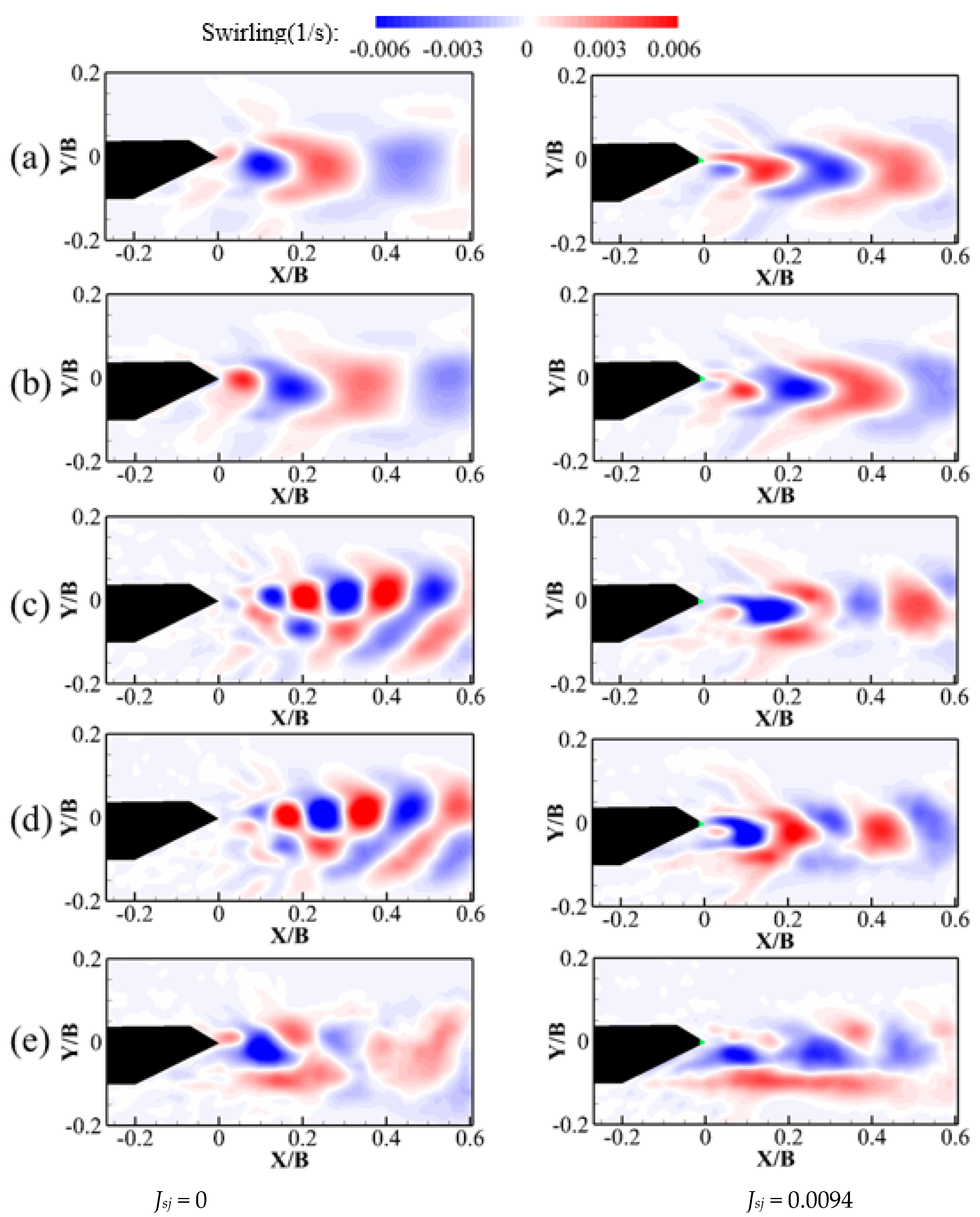
To identify the characters of the POD modes, the first five POD modes for cases J_sj = 0 and J_sj = 0.0094 are plotted in Figure 10. For the case where J_sj = 0, the first two dominant POD modes are symmetrical about the line Y/B = 0.02 and exhibit alternating vorticity that is distributed in the wake flow. Nevertheless, modes three to five vary from modes one and two: modes three and four are asymmetrical about the line Y/B = 0.02. There are two rows of counter-rotating vorticity concentrations that are displayed in the flow field behind the case J_sj = 0 closed to the test model and then changed into the arrowhead structures as the flow field moves downstream, as shown in Figure 10c,d. Moreover, mode five shows some a small-scale vorticity concentration behind case J_sj = 0. The antisymmetric vorticity flow fields that are calculated by POD represent the symmetric features of the vortex flow field. Conversely, the symmetrical vortex flow structures stand for an antisymmetric flow field, as Konstantinidis et al. [38] described. In consequence, modes one and two of the case J_sj = 0 stand for the large-scale alternating vortex shedding forming the Karman vortex street, while modes three and four denote the small spatial scale vortices with symmetric forms, and mode five represents the irregular distribution of the vorticity structures with small geometric scale. For the SBG model with the trailing edge jets, the flow structures of POD modes show noticeable differences that are in contrast to their counterparts of the uncontrolled case. The vortex concentrations of the case J_sj = 0.0094 are dramatically decreased and narrowed laterally and stretched in the flow direction, as shown in the right of Figure 10. This phenomenon of the POD modes is in connection with the elongation of the wake vortex, as shown in Figure 8b. In addition, the wake jet flow disturbs the vorticity. It divides it into two small parts at the nearing wake position as shown in modes one to four, and mode five changes to much smaller vorticity concentrating parts compared with case J_sj = 0. Based on the analysis above, the wake flow structure characteristics of the case J_sj = 0.0094 yield the unsteady aerodynamic force that is less than that of case J_sj = 0, which is consistent with the results in Section 3.2.

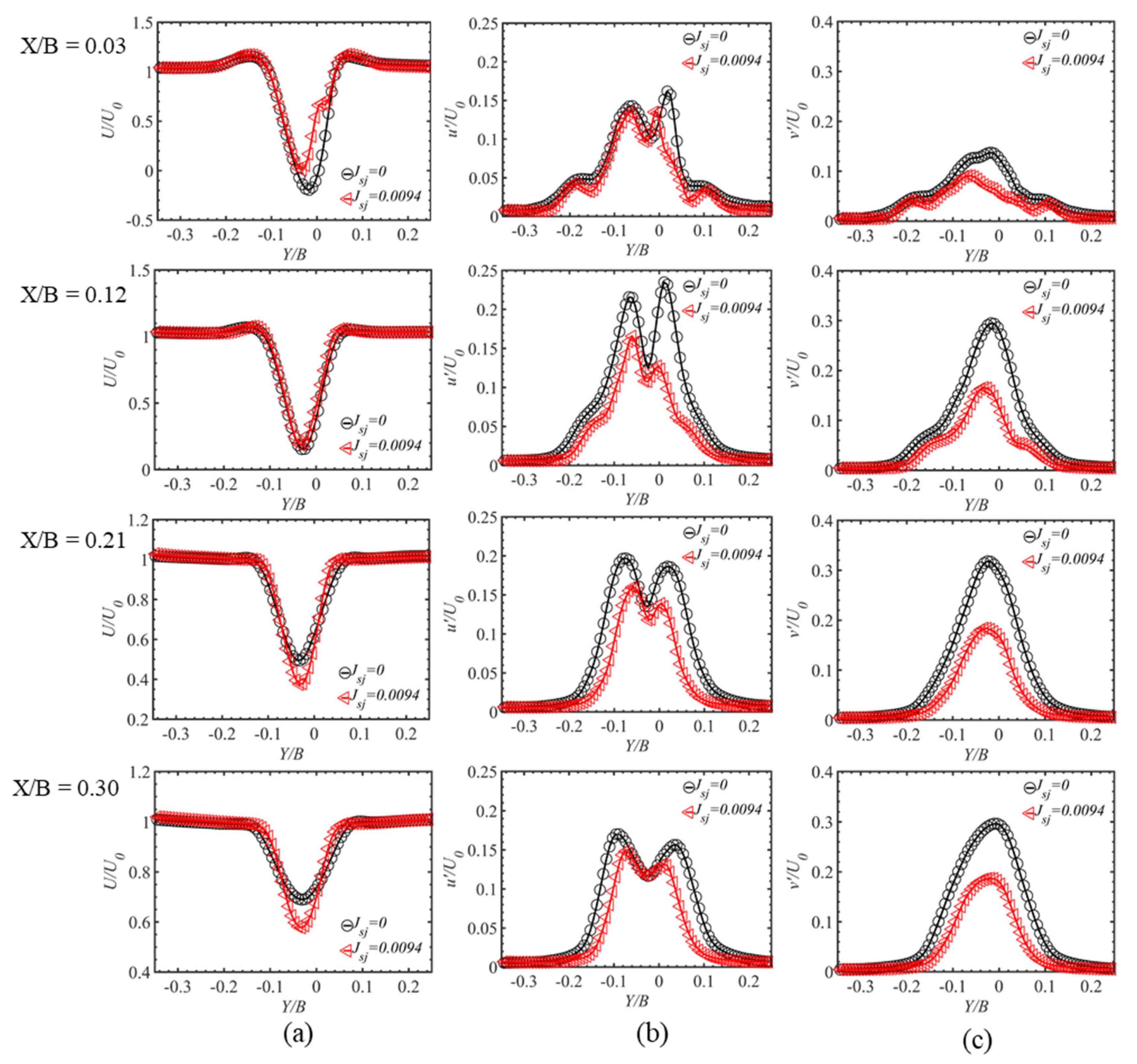
To analyze the difference of the velocity profile in the flow field behind the test model with and without the trailing edge jets, the means of the streamwise velocity, streamwise velocity fluctuation, and the transverse velocity were extracted from the PIV measurement plane I. The time-averaged streamwise velocity that was located in different positions of X/B is given in Figure 11a. The velocity profile of the case J_sj = 0 is asymmetrical in the location that is close to the SBG model and symmetrical in a further downstream position. The reason is that the geometric shape of the SBG model is asymmetrical along the line of Y/B = 0. The lowest velocity of the case J_sj = 0 was less than that of the case J_sj = 0.0094 at X/B = 0.03 and 0.12 because the jet flow can alleviate the velocity defect. That indicates the inner region flow field behind case J_sj = 0.0094 is more stable than the case J_sj = 0 [6]. Conversely, the smallest value of the velocity of the case J_sj = 0 was larger than that of case where J_sj = 0.0094 at X/B = 0.21 and 0.30. The velocity profile of the case J_sj = 0 regained faster than that of the case J_sj = 0.0094. Moreover, the width of the wake flow in case J_sj = 0 was slightly wider than the case J_sj = 0.0094, indicating the large drag force that was acting on the SBG model without control [20].

Figure 11b shows the fluctuation of the streamwise velocity profile at various positions in the wake. For the case J_sj = 0, There are two peak values that were observed in the wake flow of the case at X/B = 0.03–0.30, i.e., double-cusp mode. The maximum values appear when the turbulence level grows a dramatically quick ratio, mainly in the shear layers of the separation flow [33]. However, owing to the trailing edge jet flow disturbing the original flow field a the near-wake of X/B = 0.03, this profile for the controlled case exhibited a quadruple cusp mode. The fluctuation of the streamwise velocity profile of the case J_sj = 0.0094 presented a double-cusp mode at X/B = 0.12–0.30. It was similar to that of the case J_sj = 0, illustrating that the jet flow has a short influence range, which is identical to the investigation by Chen et al. [20]. Moreover, the peak value of the streamwise velocity fluctuation for case J_sj = 0.0094 was lower than the case J_sj = 0 at all the positions, leading to the unsteady drag force that was being exerted in the SBG model being mitigated.

The profiles of the transverse velocity fluctuation for cases J_sj = 0 and J_sj = 0.0094 are plotted in Figure 11c. The maximum value appears at approximately Y/B = 0.02, which is the axis of symmetry for the wake flow. The shear layers that are formed from the upper and lower surface are amalgamated and violently interact, causing a significant transverse velocity fluctuation [18,20]. The peak value of the case J_sj = 0 shows an increasing trend at the locations of X/B = 0.03 to 0.21 and then a reduction when X/B is more significant than 0.21, which illustrates that the shear layer interaction in the wake flow nearing to the SBG model is weaker than that of downstream. The maximum value of the fluctuation of the transverse velocity for the case J_sj = 0.0094 is obviously alleviated at all positions, indicating that the strong interaction of the shear layer decreased. That leads to the unsteady lift force that is acting on the SBG model when the trailing edge jets attenuated, as shown in Figure 5.

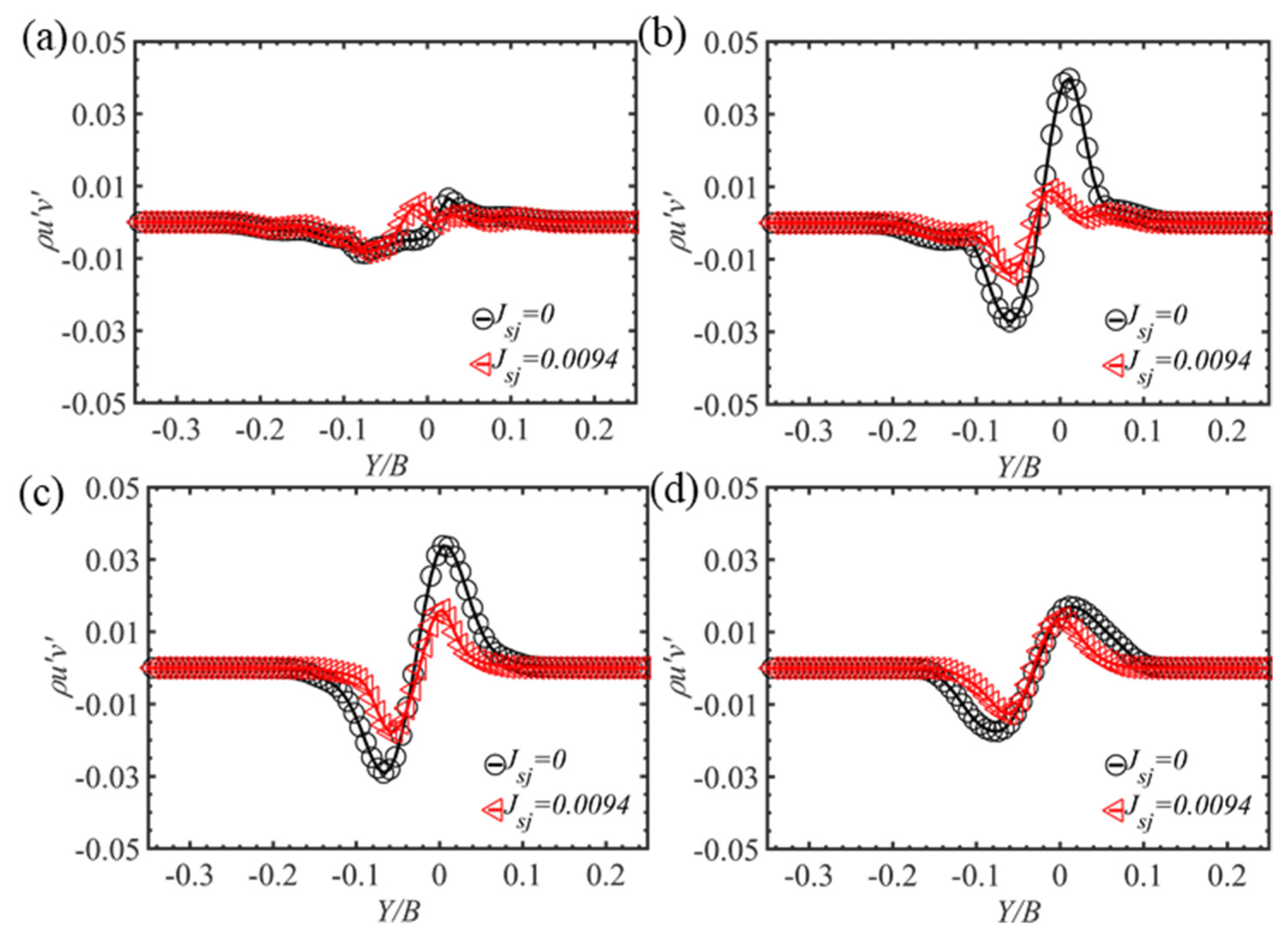
The Reynolds shear stress (RSS), which serves as an essential parameter to represent the turbulence in the flow structure, is calculated and given in Figure 12. At the near-wake of X/B = 0.03, the RSS possesses a lower value, illustrating the low turbulence level in this area for the case J_sj = 0. The maximum value of RSS is increased at first and then decreased with the improvement of the X/B. The maximum and minimum values of the RSS are obtained at the Y/B = ~−0.01 and 0.06, respectively, because the turbulence level of the shear layer that is separated from the upper and lower surface of the SBG model is strong [33]. This causes a significant fluctuation of the lift force being exerted in the SBG model. As J_sj sets as 0.0094, the RSS is mitigated at all the positions in wake flow, and the maximum and minimum values are reduced related to the uncontrolled case, which indicates that the interacting strength of the upper and lower shear layer is mitigated in the wake flow behind SBG model. Therefore, the unsteady lift force is decreased by the trailing edge jets.

3.4. Linear Stability Analysis

Triantafyllou et al. [39] found that the absolute instability of the flow field behind a bluff body is the reason for the vortex appearing in the wake of a stationary bluff body. The time-averaged streamwise velocity profiles, that were extracted from the mean flow field at various locations as shown in Figure 11a, substitute into the inviscid Orr–Sommerfeld equation (OSE). It should be noted that the higher-order small-term occurring in deducing the Orr–Sommerfeld equation and the viscidity of the air is neglected. Solving the OSE obtains the critical value in the complex frequency plane and the stability of the velocity profile by using the mathematical method that was presented by Orszag [40]. The imaginary part of the complex frequency, named as ${\omega }_i$, determines the stability of the flow structure behind the SBG model. A positive ${\omega }_i$ represents an unstable flow structure because the slight disturbance would evolve over time, leading to a large unstable flow structure [20]. Contrary, the small initial disturbance would vanish with time for a negative ${\omega }_i$. 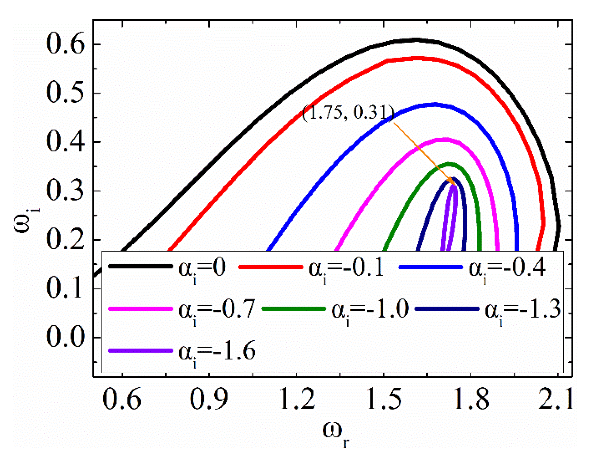Figure 13 presents the dispersion relation $\omega =\omega \left(\alpha \right)$ maps ${\alpha }_i$ constant lines on the $\omega$ plane that were obtained by solving the OSE using the velocity profile at the position X/B = 0.08 of case J_sj = 0. The $\alpha$ is the complex wave number, and the ${\alpha }_i$ is the imaginary part of $\alpha$. The imaginary and real parts of the complex frequency at the cusp point are 0.31 and 1.75, respectively. This indicates the velocity profiles behind case J_sj = 0 at X/B = 0.08 is absolute instability, causing the TKE to exhibit a considerable value in the wake flow, as shown in Figure 7a. According to the real part of $\omega$, the Strouhal number of the wake flow can be calculated as 0.28, which is close to that which is gained by using the power spectral density analysis for the lift force that is acting on the SBG model as given in Figure 6b.

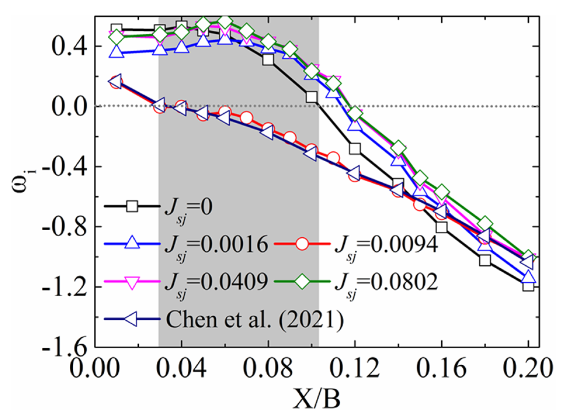
The ${\omega }_i$ at various locations behind the SBG model with and without trailing edge jets are obtained as given in Figure 14. It can be observed that the ranges of the absolute instability are stretched to the position of X/B = 0.103 for the case J_sj = 0. The flow field was slightly stable at the near-wake, and the unstable region was broader for cases J_sj = 0.0016, 0.0409, and 0.0802. However, for the case J_sj = 0.0094, the unstable area was narrowed to X/B = 0.029, indicating the unstable range decreased about 71.84% compared to that of the case J_sj = 0 as shown in the grey region of Figure 14. This phenomenon demonstrates that too strong jet flow isn’t needed for controlling the unstable flow field of the SBG model with a trailing edge jet. An appropriate jet-speed causes a steadier flow structure behind the bluff body, which is also uncovered by Gao et al. [41] in investigations of suppressing unsteady aerodynamic force that is being exerted in a circular cylinder. Therefore, a steady flow structure would excite the lower fluctuating amplitude of the aerodynamic force that is acting on the SBG model, as given in Figure 5. Moreover, the stability of the wake flow of the case J_sj = 0.0094 is similar to that of the studies of leading-edge suction and trailing-edge jet (LSTJ) that are presented by Chen et al. [20]. The superiority of the present control scheme is that the energy consumption of the case J_sj = 0.0094 is half of that of the control method of LSTJ because the present control method only needs the trailing edge jets, not the leading-edge suction.

4. Conclusions

This investigation experimentally studies the concept of trailing edge jet control to modify the vortex shedding mode for alleviating the fluctuating amplitude of surface pressure, aerodynamic force, and the unsteady flow structure. The non-dimensional jet momentum coefficient (J_sj) serves as a monitor to evaluate the strength of the wake jet flow. The surface pressure and the PIV measurements were conducted to investigate the characteristics of aerodynamic force and flow field of the single box girder (SBG) model with various J_sj. Some significant conclusions are given as follows.

The trailing edge jet that flows into the wake flow can obviously mitigate the fluctuating amplitude of the drag, lift, and moment forces. Based on the surface pressure measurement results, the saturation of the control effectiveness for lift force was obtained when the J_sj is set as 0.0094. The unsteady drag, lift, and moment forces are estimated to decrease about 16.23%, 36.34%, and 38.74%, respectively, compared to the uncontrolled case. Moreover, the vortex shedding frequency of the case J_sj = 0.0094 exhibited a difference.

The PIV measurement results explained the phenomenon that were obtained by the pressure measurement. The TKE distribution behind the SBG model with trailing edge jet were smaller than the case J_sj = 0, leading to the more stable wake. The instantaneous wake flow shows that the control method can change the antisymmetric mode into the symmetric mode, which suppresses the alternating vortex shedding and mitigates the unsteady aerodynamic force. Moreover, the unstable wake region of case J_sj = 0.0094 was narrowed by about 71.84%, compared to the uncontrolled case.