The “Skin Effect” Assessment of Chloride Ingress into Concrete Based on the Identification of Effective and Apparent Diffusivity

Abstract

The method of assessment of the “skin effect” for chloride ingress into concrete has been proposed, based on the inverse problem for the identification of at-surface variability of chloride diffusivity under fully saturated conditions. For this purpose, experimental results of 180-day diffusion tests of five types of concrete were used, which allowed the calculation of their chloride apparent diffusivity (taking into account the chloride binding by the cement matrix) and effective diffusivity (relating to the transport of free chloride ions in the pore liquid). The tested concrete samples with a water to cement ratio of 0.5 differed only in the type of cement (high early strength Portland, low-alkali normal early strength Portland, ash Portland, blast furnace, and pozzolanic). In order to effectively describe the chloride binding isotherm, a first-degree non-uniform spline function was used. Finally, the “skin effect” depth at the untreated outer surface of the concrete samples was estimated up to about 5 mm when analyzing space variability of apparent chloride diffusivity for four types of concrete with low-alkali normal early strength Portland, ash Portland, blast furnace, and pozzolanic cement. In this respect, the “skin effect” on the concrete with high early strength Portland cement was not detected.

1. Introduction

The penetration of chloride ions into concrete structures is one of the main causes of their steel reinforcement’s corrosion, especially in facilities located in the coastal zone, as well as those treated with de-icing salts. The ingress of chlorides into concrete is primarily a diffusion process taking place in the pore solution, but in general, it is more complex, and its course is also significantly influenced by the pore space structure, concentration and type of constituents dissolved in the pore liquid, interactions between chloride and other ions, age of concrete, temperature, and process of chloride binding by concrete skeleton [1]. The values of chloride diffusivity are the same influenced by the water-cement ratio, volume of aggregate, amount of cement and supplementary cementitious materials. All these factors affect the porosity of concrete, its pores’ shape and tortuosity, and ability to diffuse and bind chloride ions [2].

Chloride ions present in the hardened concrete occur in the ionic form in the pore solution (free chlorides) and are bound to the pore walls of cement matrix by the physical adsorption forces or by the chemical forces with the cement gel [3]. Initially, bound chlorides consist of insoluble salts of the MgCl_xOH_y type which, in the presence of certain additives, form hydroxy salts of the Ca(OH)₂∙CaCl₂∙2H₂O type. In addition, calcium chloride CaCl₂ reacts with the aluminate constituents of the hardened cement paste to form the so-called Friedel’s salt 3CaO∙Al₂O₃∙CaCl₂∙10H₂O, which is poorly soluble in an alkaline environment [4,5]. At normal temperature, Friedel’s salt is formed in solutions with a concentration of up to 1 g of chloride ion per 100 cm³ of solution, while at a higher concentration, unstable chloroaluminate is formed. In the case of chlorides diffusing from the outside, their binding by the C-S-H gel is difficult. However, their adsorption on the C-S-H gel surface and the formation of chloroaluminates in accordance with the pore liquid equilibrium and hydrated cement minerals is possible [6]. In the published works, the relationship between the content of bound and free chlorides is expressed with the help of mathematical relationships called binding isotherms [7]. Some researchers report a linear relationship between the content of free and bound chlorides taking into account the type of solution and its concentration [8]. However, these dependencies did not fit well to the research results in a wide range of free chloride concentrations. Therefore, non-linear relationships between the content of free and bound chlorides have been proposed. The most common are the Langmuir [9] and Freundlich [10] isotherms. The first is recommended for use with a low content of free chlorides (<0.05 mol/L), and the second with a high content (>0.01 mol/L) [11]. The isotherm proposed by Brunauer, Emmett, and Teller (BET) [12] is also used. It was found that this isotherm may fit the test results mainly when the concentration of free chloride ions is lower than 1 mol/L [13]. Some works propose completely new formulas in this regard, as in [14] where an exponential relation is introduced.

The coefficients occurring in the above-mentioned isotherms are determined experimentally using various research methods discussed in detail in [13]. In the equilibrium method, hardened cement paste samples are placed in a solution of chloride ions of known concentration and allowed to reach equilibrium. For the 10 mm thick samples, a period of up to 1 year is required. After the steady state has been achieved, the concentration of the external solution is tested by potentiometric titration. By immersing the samples in solutions of various concentrations, a graph of the adsorption isotherm is obtained. The pore solution extraction method is another one, and a complete binding isotherm may be obtained on a single specimen. However, some loosely bound chloride ions may be released into the solution under pressure. The chloride concentration could be 20% higher than the true value. In the diffusion cell method after the steady state diffusion experiment, the specimens are frozen in nitrogen and subsequently ground to powder samples [15]. The free chloride concentration is estimated by assuming that the concentration gradient is linear under steady state diffusion conditions.

It should be emphasized here that the methods discussed above are quite complicated in use, and it is also difficult to compare the research results obtained on their basis [13]. A way out of this situation is a formulation of inverse coefficient problem, in which, based on the knowledge of chloride profiles in concrete, the parameters of binding isotherms and the diffusion coefficient can be identified, minimizing a sum of square errors between the results of initial-boundary diffusion problem and experiment in non-stationary conditions [16]. Currently, models of chloride diffusion are also being developed, taking into account the division of bound chlorides into reversibly bound (as a result of physical interactions) and irreversibly bound (as a result of chemical reactions) [17,18]. For example, by splitting the bound chlorides into chemically-bound and physically-bound ones, the original problem of diffusion with chloride binding is transformed to the problem of diffusion with a moving boundary for which an analytical solution can be developed [18].

Another important issue in the analysis of chloride diffusion penetration into concrete is the so-called “skin effect” which leads to significant differences between the behaviour of concrete at the external surface up to a depth of 5–20 mm and in the bulk part of this material. Its occurrence has several reasons in practical conditions: there is the “wall effect” when pouring the concrete mix in the formwork, so that more paste and less aggregate accumulate at the surface of concrete; and/or bleeding occurs; and/or carbonation occurs; and/or brucite precipitation occurs when hydrated cement comes into contact with sea water; and/or when the concrete surface is covered with a protective layer—e.g., with paint [19]. The work of Andrade et al. [19] is one of the first to present this problem from the mathematical point of view where the modification of the classical model of chloride diffusion in a half-space is proposed, taking into account two layers with different apparent diffusion coefficients. The “skin effect” may also arise in the case of chloride diffusion under unsaturated conditions in the pores of concrete, and then it typically consists in shifting the maximum concentration of chloride under the concrete surface due to the alternating phenomena of moistening and drying, washing out chlorides from the surface by rainfall, etc. [20]. Therefore, the effective prediction of the progress of chloride penetration into concrete and the assessment of the durability of reinforced concrete structures from this point of view should take into account this effect depending on the method of surface finishing.

An unequivocal evaluation of the process and the related selection of appropriate concrete durability models is further complicated by the fact that the penetration of chlorides into concrete depends on the additives of waste materials to cements commonly used today. For example, based on [13], it can be stated that adding ground granulated blast furnace slag or fly ash to cement increases the chloride binding capacity while adding silica fume decreases it.

Taking into account the facts discussed above, the authors, to the best of their knowledge, did not find in the literature review an attempt to identify the binding isotherm parameters together with the diffusion coefficient for chlorides in concrete based on the knowledge of their profiles from diffusion tests, which will lead to a quantitative assessment of the “skin effect” including different types of cement. For this purpose in following Section 2 and Section 3 of the article, the experiment and the mathematical model that enables such estimation are presented in detail. In the experimental part, five types of concrete were taken into account by the authors, different in their recipe only due to the binder (high early strength Portland, low-alkali normal early strength Portland, ash Portland, blast furnace, and pozzolanic cement) [21], and in the sense of concrete constituents’ impact on the process, the current research should be regarded as preliminary and restricted to the selected types of cement. On the basis of experimental curves (showing 180-day distributions of diffusing chlorides in 2 mm layers up to 2 cm depth of samples with untreated surfaces which were exposed to a 3% NaCl solution under fully saturated conditions), the binding isotherms and the effective and apparent chloride diffusion coefficients were estimated. In order to effectively assess the “skin effect” using the mentioned quantities, the authors proposed a first-degree non-uniform spline to describe the binding isotherms, and the identification of material parameters based on minimizing the objective function in the form of a sum of errors between the results from the diffusion model and experiment. The latter was achieved following the previous experiences of one of the authors gained in the course of works published in [22,23]. Finally, the “skin effect” depth at the untreated outer surface of the concrete samples was estimated up to about 5 mm on the basis of space variability of apparent chloride diffusivity depending on the type of cement used, which was described in detail in Section 4 and summarized in Section 5.

2. Experimental Results

The experimental results presented below have already been partially described in the works of one of the authors [21] (for concretes denoted further as C1 and C3–C5), but without a detailed analysis of the diffusion of free chlorides and their binding by the concrete skeleton in the context of the “skin effect” assessment, which was carried out only for the purposes of this article. Due to the importance of the sample preparation and testing methods (influencing the formulation of the mathematical model—see Section 3), the authors decided to briefly describe the experimental work used in the study as bellow.

In this work, the test results of testing 5 types of normal concrete were used marked as C1–C5. Three types of natural rounded aggregate from Lafarge Basalt Mine in Lubień (Poland) compliant with the standard PN-EN 12620 [24], i.e., sand (0–2 mm) and gravel (2–8 mm and 8–16 mm), and five types of cement produced according to PN-EN 197-1 [25] at the Lafarge cement plant in Małogoszcz (Poland) were used for the concrete mixes. The following types of cements (with the standard denotations according to [25]) were used: Portland cement of high early strength (CEM I 42.5 R) in concrete C1, ash Portland cement (CEM II/B-V 32.5 R) in concrete C2, blast furnace cement (CEM III/A 32.5 N-LH/HSR/NA) in concrete C3, low-alkali Portland cement of normal early strength (CEM I 42.5 N-SR3/NA) in concrete C4, and pozzolanic cement (CEM IV/B (V) 32.5 R-LH/NA) in concrete C5. Their detailed chemical composition and basic properties (according to the producer’s specification) are given in

Table 1. Chemical composition and selected properties of cements according to the producer’s specification. The denotations used in the table: CEM I—Portland cement; CEM II—multi-component Portland cement; CEM III—blast furnace cement; CEM IV—pozzolanic cement; for CEM II/B, CEM III/A, and CEM IV/B, maximum contents of non-clinker principal components are in mass percentages: 35, 65, and 55, respectively; R—high early strength cement; L—low early strength cement; N—normal early strength cement; NA—low-alkali cement; HSR—sulphate-resistant cement, SR3—sulphate-resistant cement with a tricalcium silicate content of not more than 3 mass percentages; LH—cement with low heat of hydration (data also partially published in [21]).

Parameters		CEM I 42.5 R	CEM II/B-V 32.5 R	CEM III/A 42.5 N-LH/HSR/NA	CEM I 42.5 N/SR3/NA	CEM IV/B (V) 32.5 R-LH/NA
Constituents	SiO2	19.38	26.77	29.08	21.15	30.18
in weight (%)	Al2O3	4.57	10.82	6.30	3.93	11.92
	Fe2O3	3.59	3.97	1.37	5.14	4.72
	CaO	63.78	45.91	48.82	63.34	41.95
	MgO	1.38	1.62	4.36	1.28	1.72
	K2O	0.58	1.42	0.73	0.39	1.43
	Na2O	0.21	1.30	0.34	0.21	0.39
	Eq. Na2O	0.59	1.25	0.82	0.47	1.33
	SO3	3.26	2.77	2.74	2.61	2.65
	Cl	0.069	0.08	0.066	0.058	0.057
Surface (cm2/g)		3535	3500	4760	3067	4457
Density (g/cm3)		3.09	2.78	2.97	3.18	2.65
Setting time (min)	beginning	160	262	238	210	200
	end	200	382	293	255	290
Compression	2 days	30.3	18.0	14.9	24.7	20.9
strength (MPa)	28 days	56.9	45.2	57.6	54.1	43.2
Water demand (%)		27.6	29.8	31.6	27.8	29.0

, and the detailed compositions of concrete mixes C1–C5 are presented in

Table 2. The composition of concrete mixtures (data also partially published in [21]).

Concrete	Type of Cement	Cement (kg/m3)	Sand (kg/m3)	Gravel (kg/m3)	Water to Cement Ratio
C1	CEM I 42.5 R	324	738	1193	0.5
C2	CEM II/B-V 32.5 R
C3	CEM III/A 42.5 N-LH/HSR/NA
C4	CEM I 42.5 N-SR3/NA
C5	CEM IV/B (V) 32.5 R-LH/NA

.

In order to establish the basic hardened concrete properties, the tests of concretes C1–C5 were performed at the Laboratory of Civil Engineering of the Silesian University of Technology. The compressive strength was tested on 6 samples of 150 mm cubes for every type of concrete after 28 days moist curing according to PN-EN 12390-3 [26]. In order to determine the open porosity of hardened concrete, the following scheme was used: 1 sample for every type of concrete with a volume of about 10 cm³, after 90 days of maturation under water, was placed in an oven at 60 °C, and its mass was measured daily. When the mass of the sample differed on two consecutive days less than 0.1%, it was regarded as being in a dry state. Then the sample was saturated with water again by immersion to the moment its mass on two consecutive days was the same. Next, the floating weight of the sample was measured with the use of hydrostatic laboratory balance. Finally, the open porosity of the samples, ε (m³/m³), was calculated according to the following equation:

$$\epsilon =\frac{m_{\mathrm{S}}-m_{\mathrm{D}}}{m_{\mathrm{S}}-m_{\mathrm{FS}}}$$

(1)

where: $m_{\mathrm{S}}$—mass of the sample (kg) after the water re-saturation, $m_{\mathrm{D}}$—mass of the sample (kg) in the dry state, $m_{\mathrm{FS}}$—floating weight of the sample (kg) after the water re-saturation. The average compressive strength, apparent density, and porosity of the tested concretes are presented in

Table 3. Mean compressive strength ($f_{\mathrm{cm}}$), bulk density (${\rho }_{\mathrm{b}}$), and open porosity ($\epsilon$) of tested concretes (data also partially published in [21]).

Concrete	fcm (MPa)	$\mathit{\rho }$ (kg/m3)	$\mathit{\epsilon }$ (m3/m3)
C1	54.2	2271	0.12
C2	45.8	2241	0.10
C3	49.5	2269	0.07
C4	58.4	2258	0.09
C5	46.5	2280	0.10

.

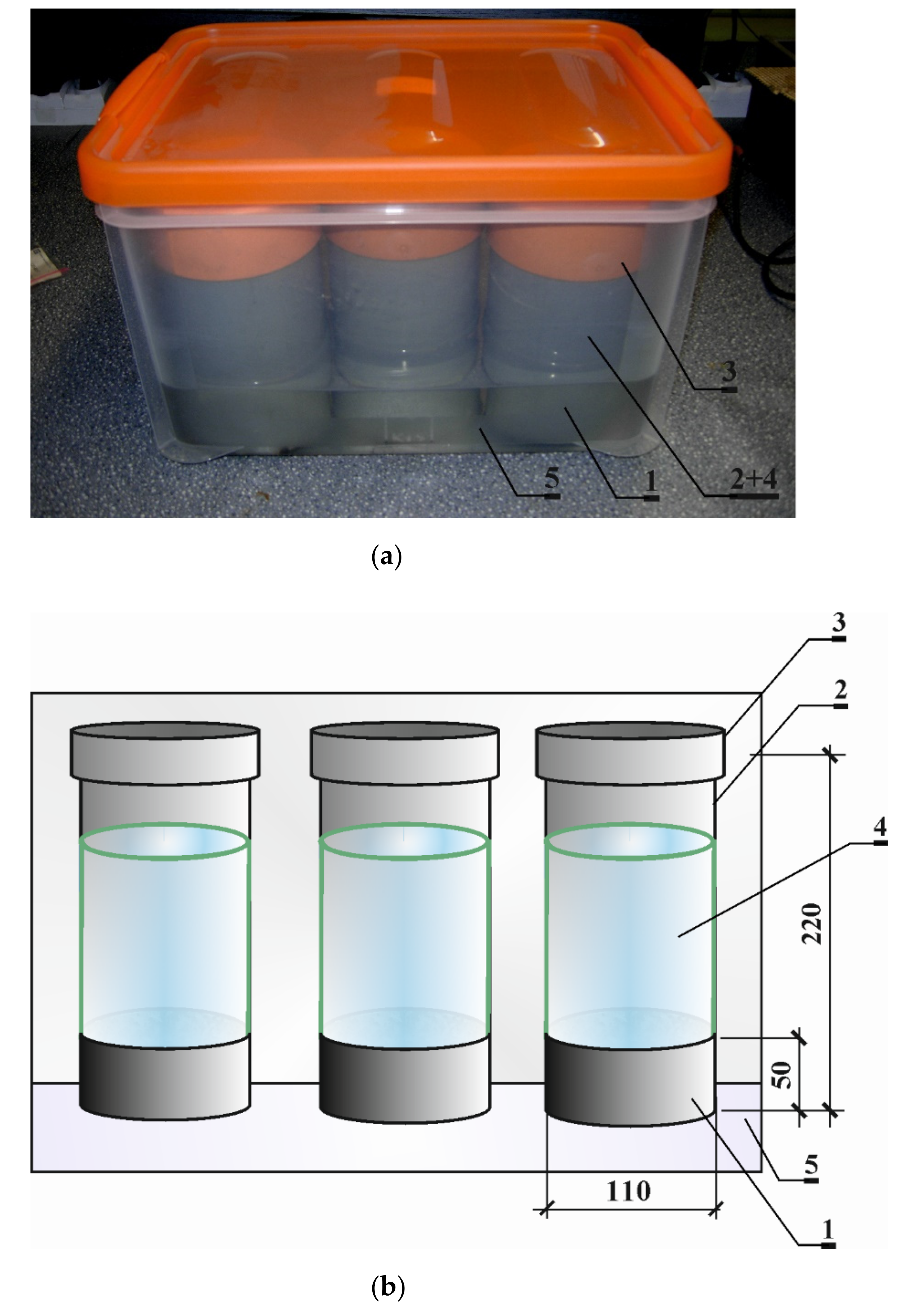
The chloride ion diffusion tests were also carried out at the Laboratory of Civil Engineering of the Silesian University of Technology. They were performed for every type of concrete on three cylinder-shaped samples with a diameter of 100 mm and a height of 50 mm. The concrete samples were poured into the cutouts of plastic pipes that provided them with the aforementioned dimensions. The visible surfaces of samples were untreated after setting so as to obtain a typical surface of concrete exposed to chlorides under practical conditions from the top of a concrete member and to be able to assess the chloride diffusion “skin effect” in this case. After they had matured for 28 days under water, they were stored at the room conditions. Prior the diffusion tests, they were re-saturated again with distilled water by immersion until they reached constant mass. The initial preparation of the samples was carried out so that the diffusion tests could begin 90 days after the concrete had set. In order to force unidirectional diffusion transport of chloride ions in the samples, 3% solution of NaCl was placed in the containers attached with waterproof glue to the top surface of the plastic pipes confining the concrete samples, and the bottom surfaces of samples were placed in distilled water. 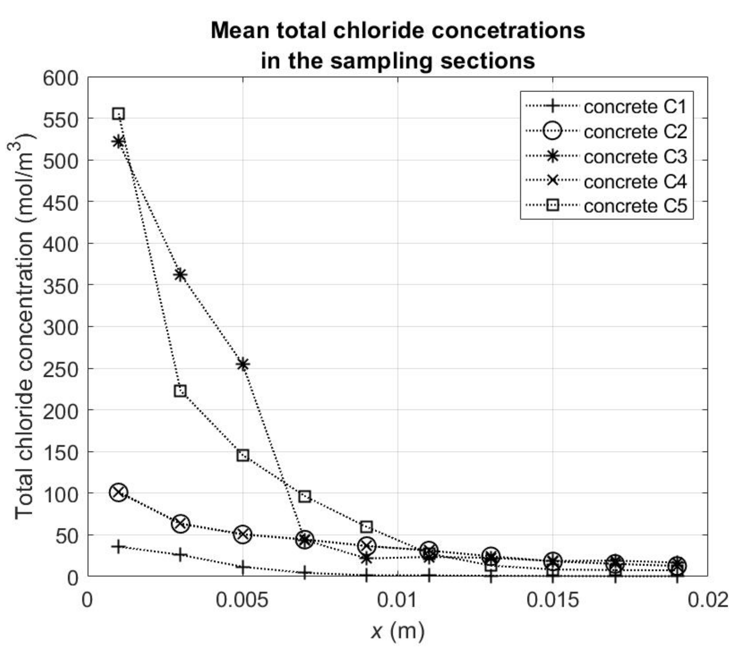The photo of the diffusion test stand and its diagram are presented in Figure 1. The test was carried out at the temperature about 20 °C. It was carried out during 180 days from the beginning of the chloride diffusion process. As a result, curves describing the mean total (i.e., free and bound) chloride ions concentration in 2 mm sampling sections to a 2 cm depth of concrete samples were obtained (

Table 4. Mean concentration of chlorides in the washed solution ($c_{\mathrm{sol}}$), mean volumetric concentration of total chlorides (${\overline{C}}_{\mathrm{t}\exp }$) in concrete, and mass percentage of chlorides in relation to the cement mass per a unit volume of concrete ($p$) determined for the 2 mm sampling sections from the drill holes. Coordinate $x=0$ relates to the specimen external surface exposed to the chloride solution (data also partially published in [21]).

Concrete	Coordinates of Sampling Sections x (mm)	${\mathit{c}}_{\mathbf{sol}}$ (mg/m3)	${\overline{\mathit{C}}}_{\mathbf{t} \mathbf{exp}}$ (mol/m3)	$\mathit{p}$ (%)
C1	0–2	280	35.9	0.39
	2–4	203	26.0	0.28
	4–6	91.0	11.7	0.13
	6–8	34.2	4.38	0.048
	8–10	12.0	1.54	0.017
	10–12	10.8	1.39	0.015
	12–14	7.49	0.96	0.010
	14–16	5.23	0.67	0.007
	16–18	3.22	0.41	0.005
	18–20	2.95	0.38	0.004
C2	0–2	670	101	1.10
	2–4	592	63.2	0.69
	4–6	668	50.4	0.55
	6–8	606	44.2	0.48
	8–10	430	36.5	0.40
	10–12	317	31.1	0.34
	12–14	255	24.2	0.26
	14–16	134	18.1	0.20
	16–18	74.5	15.2	0.17
	18–20	27.0	12.6	0.14
C3	0–2	4076	522	5.71
	2–4	2832	363	3.97
	4–6	1990	255	2.79
	6–8	342	43.7	0.48
	8–10	169	21.7	0.24
	10–12	184	23.5	0.26
	12–14	175	22.4	0.24
	14–16	146	18.7	0.20
	16–18	149	19.1	0.21
	18–20	131	16.8	0.18
C4	0–2	798	102	1.11
	2–4	500	63.7	0.70
	4–6	399	50.8	0.56
	6–8	350	44.6	0.49
	8–10	289	36.8	0.40
	10–12	246	31.3	0.34
	12–14	191	24.4	0.27
	14–16	143	18.2	0.20
	16–18	120	15.3	0.17
	18–20	100	12.7	0.14
C5	0–2	4320	556	6.08
	2–4	1734	223	2.44
	4–6	1134	146	1.60
	6–8	750	96.5	1.05
	8–10	462	59.4	0.65
	10–12	216	27.8	0.30
	12–14	102	13.1	0.14
	14–16	66.0	8.49	0.093
	16–18	60.0	7.72	0.084
	18–20	58.0	7.46	0.082

). One resulting concentration curve was prepared based on the averaged values from three samples made of the same concrete (Figure 2). The mean chloride ion concentration in each section was obtained after rinsing chloride ions from the powdered concrete with distilled water. One sample of powdered concrete was washed two times (each time with water in amount which was in mass equal to mass of powdered concrete sample). The powdered concrete material was obtained by using a drilling rig with a diamond drill “Profile Grinding Kit” produced by German Instruments AS. The concentrations of chloride ions obtained from the chemical analysis of the tested solutions were then converted into the mean volumetric concentrations in the concrete 2 mm sampling sections of total chlorides ions (${\overline{C}}_{\mathrm{t}\exp }$ (mol/m³)) and their concentrations ($p$ (%)) expressed for reference as a percentage of the cement mass per a concrete unit volume according to the following formulas:

$${\overline{C}}_{\mathrm{t} \exp }=\frac{m_{\mathrm{t} \exp }}{M_{\mathrm{Cl}}{V}_{\mathrm{c}}}=\frac{2 c_{\mathrm{sol}}·{\rho }_{\mathrm{cb}}}{M_{\mathrm{Cl}}{\rho }_{\mathrm{w}}}, p=\frac{{\overline{C}}_{\mathrm{t} \exp }·M_{\mathrm{Cl}}}{{\rho }_{\mathrm{cem}}}·100\%$$

(2)

where: $c_{\mathrm{sol}}—$ chloride ion concentration (kg/m³) determined in the washed solution, $m_{\mathrm{t}\exp }$—mass of total chlorides (kg) in the powdered concrete drilled from a sampling section, $V_{\mathrm{c}}$—volume of the drilled concrete (m³) from sampling section in an intact state, ${\rho }_{\mathrm{cb}}$—bulk density (kg/m³) of concrete, $M_{\mathrm{Cl}}=0.035453$ kg/mol—molar mass of chloride, ${\rho }_{\mathrm{w}}$ = 1000 kg/m³—density of water, ${\rho }_{\mathrm{cem}}$—density of cement (kg/m³) per a concrete unit volume. The precise details of the used experimental and calculation procedure for the determination of ${\overline{C}}_{\mathrm{t}\exp }$ can be found in article [27].

3. Mathematical Model

The mathematical model was formulated taking into account the basic objectives of the research (Section 1) and the conditions of the experiment (Section 2). It was assumed that the transport of chloride ions in concrete under fully saturated conditions at constant temperature can be described by the following system of two local mass balances—respectively for the free chloride ions in the pore liquid and chlorides bound by the concrete skeleton (without distinction to chemically or physically bound chlorides):

$$\epsilon M_{\mathrm{Cl}}\frac{\partial C_{\mathrm{f}}}{\partial t}=-\epsilon \nabla ∆j_{\mathrm{f}}-\left(1-\epsilon \right) S,$$

(3)

$$M_{\mathrm{Cl}}\frac{\partial C_{\mathrm{b}}}{\partial t}=S$$

(4)

where: $C_{\mathrm{f}}$—concentration of free chlorides (mol/m³), $C_{\mathrm{b}}$—concentration of bound chlorides (mol/m³), $j_{\mathrm{f}}$—vector of free chloride mass flux density (kg/(s·m²)) in the pore liquid, $S$—density of the mass source of bound chlorides (kg/(s·m³)) in the concrete skeleton, $\nabla$—nabla operator (1/m), $t$—time (s). The form of mass balance (4) for the bound chlorides corresponds to the situation in which it is assumed that the adsorption of chlorides by the skeleton is so fast compared to the diffusion process that it can be considered immediate. If the function of the chloride binding isotherm is known:

$$C_{\mathrm{b}}=f\left(C_{\mathrm{f}}\right),$$

(5)

and in addition, we can assume the isotropy of the material, the isothermality of the process, and take into account the diffusion of free chlorides using I Fick’s law with an effective diffusion coefficient independent of the chloride concentration, i.e.,

$$j_{\mathrm{f}}=-D_{\mathrm{eff}} M_{\mathrm{Cl}}\nabla C_{\mathrm{f}}$$

(6)

where: $D_{\mathrm{eff}}$—effective constant diffusion coefficient in (m²/s), then we can obtain the following differential equation based on the mass balances (3) and (4):

$$\frac{\partial C_{\mathrm{f}}}{\partial t}=\frac{\epsilon D_{\mathrm{eff}}}{\epsilon +\left(1-\epsilon \right)\frac{\partial C_{\mathrm{b}}}{\partial C_{\mathrm{f}}}}{\nabla }^2{C}_{\mathrm{f}}.$$

(7)

Equation (7) can also be presented as:

$$\frac{\partial C_{\mathrm{f}}}{\partial t}=D_{\mathrm{app}}{\nabla }^2{C}_{\mathrm{f}}$$

(8)

where:

$$D_{\mathrm{app}}\left(C_{\mathrm{f}}\right)=\frac{\epsilon D_{\mathrm{eff}}}{\epsilon +\left(1-\epsilon \right)\frac{\partial C_{\mathrm{b}}}{\partial C_{\mathrm{f}}}} ,$$

(9)

is the apparent chloride diffusion coefficient in (m²/s), generally dependent on the concentration of free chlorides and taking into account the process of binding them in the skeleton. Equation (8) in the case of one-dimensional diffusion transport will simplify to the form:

$$\frac{\partial C_{\mathrm{f}}}{\partial t}=D_{\mathrm{app}}\frac{{\partial }^2{C}_{\mathrm{f}}}{\partial x^2}$$

(10)

where: $x$—spatial variable (m). When maintaining a concrete sample in a water solution with a known and constant concentration of chlorides, $C_{\mathrm{fe}}$, on one of its ends (when $C_{\mathrm{f}}\left(x=0,t\right)=C_{\mathrm{fe}}$), with the initial zero concentration of chlorides (when $C_{\mathrm{f}}\left(x,t=0\right)=C_{\mathrm{f}0}=0$), and assuming a linear approximation of the binding isotherm (5), i.e.,

$$C_{\mathrm{b}}=a C_{\mathrm{f}}$$

(11)

where: a—slope (-) of a linear isotherm, a well-known analytical solution of Equation (10) [28] can be obtained:

$$C_{\mathrm{f}}=C_{\mathrm{fe}}\left(1-\mathrm{erf}\left(\frac{x}{2\sqrt{D_{\mathrm{app}}t}}\right)\right)$$

(12)

where in this case:

$$D_{\mathrm{app}}=\frac{\epsilon D_{\mathrm{eff}}}{\epsilon +\left(1-\epsilon \right)a}.$$

(13)

The solution (12) is valid for the half-space, $x\ge 0$, and as such can be used to a suitable approximation for modelling the concrete chloride saturation process in the initial phase of the experiment. Of course, if $D_{\mathrm{app}}$ has a non-linear course, an approximate solution of Equation (10) is possible without much difficulty using the Finite Difference Method (FDM), which was also used in this article. Using an explicit scheme in the time discretization of the problem and equidistant nodal points in the space discretization, we can calculate for a sample of length $l$ (m) that:

$$C_{\mathrm{f}}\left(x_i,t_j+∆t\right)=D_{\mathrm{app}}\left(C_{\mathrm{f}}\left(x_i,t_j\right)\right)·\frac{C_{\mathrm{f}}\left(x_i-∆x,t_j\right)-2C_{\mathrm{f}}\left(x_i,t_j\right)+C_{\mathrm{f}}\left(x_i+∆x,t_j\right)}{∆x^2}·∆t+C_{\mathrm{f}}\left(x_i,t_j\right)$$

(14)

where: $i=1,2,\dots ,m$—node index; $j$ = 1, 2, …—index of the moment; $m$—number of nodes; $x_i$—coordinate (m) of the $i$-th node where $x_1=0$ and $x_m=l$; $t_j$—the $j$-th moment (s) where $t_1=0$; $∆x$—distance (m) between nodes where $∆x=l/\left(m-1\right)$; $∆t$—time step (s). At the zero initial concentration (i.e., $C_{\mathrm{f}}\left(x,0\right)=C_{\mathrm{f}0}=0$), when maintaining a concrete sample in a solution of known and constant chloride concentration, $C_{\mathrm{fe}}$, at one of its ends (i.e., $C_{\mathrm{f}}\left(0,t\right)=C_{\mathrm{fe}}$) and in distilled water at the other of its ends (i.e., $C_{\mathrm{f}}\left(l,t\right)=0$), it is assumed in Equation (14) that:

$$C_{\mathrm{f}}\left(x_1,t_j\right)=C_{\mathrm{fe}}\mathrm{and}{C}_{\mathrm{f}}\left(x_m,t_j\right)=0\mathrm{for}j=1,2,\dots ,$$

(15)

$$C_{\mathrm{f}}\left(x_i,t_1\right)=C_{\mathrm{f}0}\mathrm{for}i=1,2,\dots ,m.$$

(16)

In order to ensure the convergence of the solution due to the discretization in the time domain in the calculations presented further, $∆t$ was determined at each $j$-th time step so that the two conditions were met:

$$∆t\le 0.01\frac{∆x^2}{\max {\left(D_{\mathrm{app}}\left(C_{\mathrm{f}}\left(x_i,t_j\right)\right)\right)}_{i=1,2,\dots ,m}},$$

(17)

$$\max {\left(C_{\mathrm{f}}\left(x_i,t_j+∆t\right)-C_{\mathrm{f}}\left(x_i,t_j\right)\right)}_{i=1,2,\dots ,m}\le 0.01\left(C_{\mathrm{fe}}-C_{\mathrm{f}0}\right).$$

(18)

After solving Equation (10), the concentration of total chlorides can be estimated from the equation:

$$C_{\mathrm{t}}=\epsilon C_{\mathrm{f}}+\left(1-\epsilon \right) C_{\mathrm{b}}=\epsilon C_{\mathrm{f}}+\left(1-\epsilon \right) f\left(C_{\mathrm{f}}\right).$$

(19)

The presented mathematical description of the chloride transport process in concrete, which comes down to the differential Equation (10) with a constant $D_{\mathrm{app}}$ coefficient, is widely used in the literature directly or with some modifications resulting from the specificity of the chloride diffusion process [19,20]. This is because of the ease of its use and the interpretation of experimental results under fully saturated conditions, where analytical solutions can be used. However, after taking into account the dependencies (5), (9), and (19), the presented mathematical description also makes it possible to take into account the binding intensity of free chlorides in the concrete skeleton depending on their concentration. Then, in Equation (5), the most common is a form of the linear [16,29] (giving the constant $D_{\mathrm{app}}$ in the range of the considered variability of free chloride concentration), Langmuir [16,29,30,31], BET [13], or Freundlich isotherm [16,29,30,31]:

$$\begin{gathered} \mathrm{Linear}:C_{\mathrm{b}}=a C_{\mathrm{f}},\mathrm{Langmuir}:C_{\mathrm{b}}=\frac{a_{\mathrm{L}}{C}_{\mathrm{f}}}{1+b_{\mathrm{L}}{C}_{\mathrm{f}}}, \\ \mathrm{BET}:C_{\mathrm{b}}=\frac{a_{\mathrm{BET}} b_{\mathrm{BET} }{C}_{\mathrm{f}}}{\left(C_{\mathrm{f}\max }-C_{\mathrm{f}}\right)\left(1+\left(b_{\mathrm{BET}}-1\right) \frac{C_{\mathrm{f}}}{C_{\mathrm{f}\max }}\right)},\mathrm{Freundlich}:C_{\mathrm{b}}=a_{\mathrm{F}}{C}_{\mathrm{f}}^k, \end{gathered}$$

(20)

where: $a$, $a_{\mathrm{L}}$, $a_{\mathrm{BET}}$, $a_{\mathrm{F}}$, $b_{\mathrm{L}}$, $b_{\mathrm{BET}}$, $k<1$—parameters characterizing the process, $C_{\mathrm{f}\max }$—maximum concentration of free chlorides in solution (mol/m³). The first is simply a convenient form of approximating the physical relationship, the second and the third assume that the gas-phase adsorbate layer on the solid adsorbent is a monolayer [9] or poly-layer [12], and the fourth is empirical [10]. The Langmuir and BET ones are originally formulated for the physical process of different nature in comparison to the binding chlorides by the cement matrix, and they should be used in the description of the considered process with some restrictions concerning its interpretation. The BET isotherm has an inflection point from negative to positive curvature where the curvature is negative for lower concentrations and positive for higher concentrations, however, the isotherm itself may significantly overestimate the result in the area of $C_{\mathrm{f}}$ concentrations close to $C_{\mathrm{f}\max }$, which results from the term $\left(C_{\mathrm{f}\max }-C_{\mathrm{f}}\right)$ in its denominator. The course of the Langmuir and Freundlich isotherms is characterized by a negative curvature in the entire range of the $C_{\mathrm{f}}$ variability under consideration, which agrees quite well with a number of experimental data for different types of concrete available in the literature (e.g., [29,30,32]). These data, in order to be representative for cement matrix materials, are obtained from tests of chloride binding by material taken from the internal parts of samples [29,32] or from fully ground samples [30]. In this way, the influence of a different structure of the boundary layer of the samples on the results, in which the proportion of cement paste and aggregate or porosity may be changed, is compensated. For example, interesting structural studies of the external layer of concrete samples with different surface treating methods are presented in [33]. Due to the fact that in practical conditions, the external parts of concrete elements are obviously not removed and mediate the transport of chlorides to the interior of the concrete, the determination of the chloride binding isotherms taking into account the influence of the near-surface layers is an important issue. In the literature, this phenomenon is referred to as the “skin effect”, which was described in more detail at the beginning of the article. An appropriate correction of the mathematical model from this point of view is of great importance in correctly predicting the progress of chloride transport in reinforced concrete structures, the more so as the typical thicknesses of the concrete cover of steel reinforcement are up to 5 cm, and the thicknesses of the surface zones with changed properties may be of the order of the thickest aggregate fraction radius. Thus, it follows that the thicknesses of the zones affecting the “skin effect” may be of the same order as the thickness of the reinforcement cover. With the above in mind, the authors limited themselves to analyzing the “skin effect” under the following extent and simplifying assumptions:

(1)

The conditions of the experiment should emphasize in the transport of chlorides only the influence of the change in the composition and structure of concrete in the near-surface part in relation to the bulk part (i.e., due to the increase in the volume of cement paste in relation to the aggregate and/or the change in porosity).

(2)

The most simple mathematical model should be chosen for the description of the phenomenon, bearing in mind the limitation of the number of identified parameters to the necessary minimum and obtaining the best possible conditioning of the coefficient inverse problem, but with the possibility of a reasonable quantification of the effect.

Due to the first assumption, the surface layers must not be removed from the samples before the chloride diffusion process was started, and the experiment should be conducted in the isothermal and saturated conditions on concrete samples of at least 90 days to avoid excessive hydration process impact on the process. At the same time, the experiment should last long enough to capture changes in the concentration distribution as much as possible, but also as short as possible to limit the impact of hydration of cement relics in concrete skeleton on changes in the diffusion coefficient (e.g., [1]). Hence, the authors decided to use the research of the diffusion process lasting 180 days from its start which was described in Section 2. 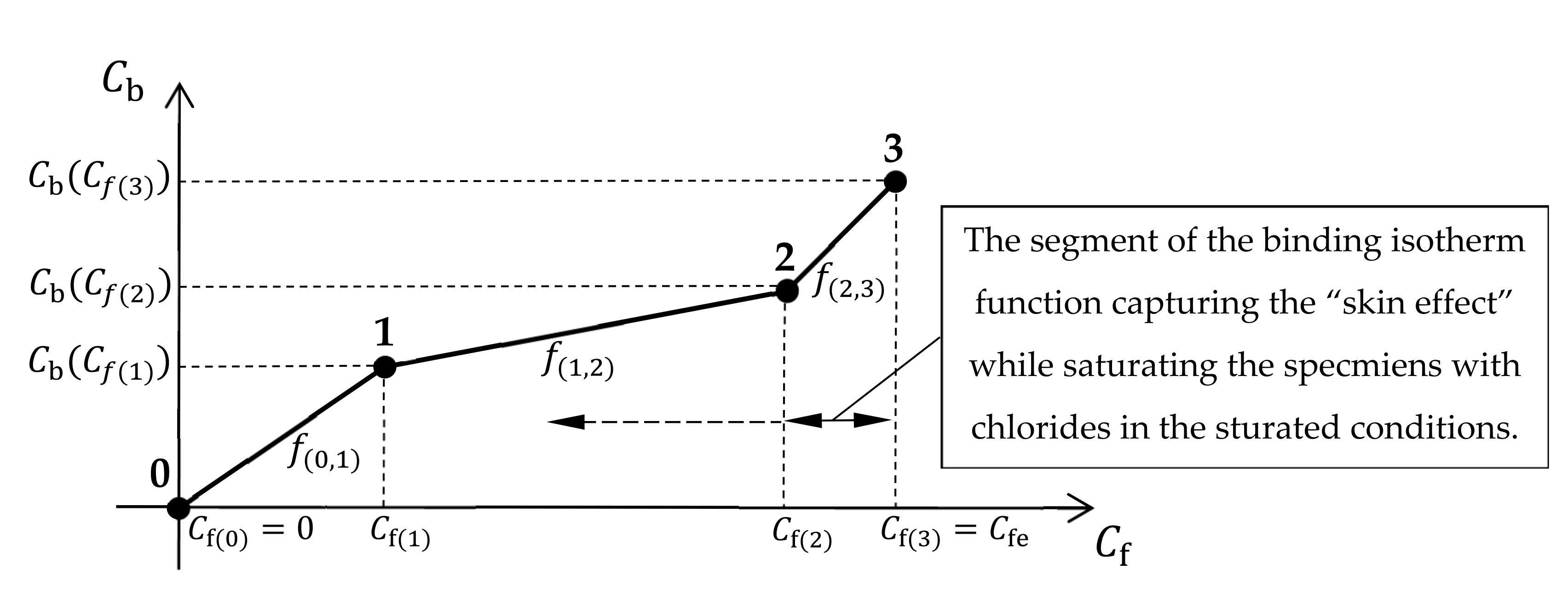Moreover, since the binding effect strongly depends on the cement composition [32], the data for the samples with different composition depending on the used type of binder were the same selected. Due to the second assumption in the article, it is proposed to use the mathematical model described above in which the first-degree non-uniform spline function will be used to approximate the relationship (5) in the form:

$$C_{\mathrm{b}}=\left\{\begin{array}{c}{f}_{\left(0,1\right)}\left(C_{\mathrm{f}}\right)=a_{\left(1\right)}{C}_{\mathrm{f}}+b_{\left(1\right)} \mathrm{for} C_{\mathrm{f}}\in \left[C_{\mathrm{f}\left(0\right)}\right.,\left.C_{\mathrm{f}\left(1\right)}\right]\\ f_{\left(1,2\right)}\left(C_{\mathrm{f}}\right)=a_{\left(2\right)}{C}_{\mathrm{f}}+b_{\left(2\right)} \mathrm{for} C_{\mathrm{f}}\in \left[C_{\mathrm{f}\left(1\right)}\right.,\left.C_{\mathrm{f}\left(2\right)}\right]\\ ⋮\\ f_{\left(i-1,i\right)}\left(C_{\mathrm{f}}\right)=a_{\left(i\right)}{C}_{\mathrm{f}}+b_{\left(i\right)} \mathrm{for} C_{\mathrm{f}}\in \left[C_{\mathrm{f}\left(i-1\right)}\right.,\left.C_{\mathrm{f}\left(i\right)}\right]\\ ⋮\\ f_{\left(n-1,n\right)}\left(C_{\mathrm{f}}\right)=a_{\left(n\right)}{C}_{\mathrm{f}}+b_{\left(n\right)} \mathrm{for} C_{\mathrm{f}}\in \left[C_{\mathrm{f}\left(n-1\right)}\right.,\left.C_{\mathrm{f}\left(n\right)}\right]\end{array}\right.$$

(21)

where:

$$a_{\left(i\right)}=\frac{C_{\mathrm{b}}\left(C_{\mathrm{f}\left(i\right)}\right)-C_{\mathrm{b}}\left(C_{\mathrm{f}\left(i-1\right)}\right)}{C_{\mathrm{f}\left(i\right)}-C_{\mathrm{f}\left(i-1\right)}},b_{\left(i\right)}=\frac{C_{\mathrm{f}\left(i\right)}·C_{\mathrm{b}}\left(C_{\mathrm{f}\left(i-1\right)}\right)-C_{\mathrm{f}\left(i-1\right)}·C_{\mathrm{b}}\left(C_{\mathrm{f}\left(i\right)}\right)}{C_{\mathrm{f}\left(i\right)}-C_{\mathrm{f}\left(i-1\right)}},$$

(22)

$i=1,2,\dots ,n$; $C_{\mathrm{f}\left(0\right)}=0<C_{\mathrm{f}\left(1\right)}<C_{\mathrm{f}\left(2\right)}<\dots <C_{\mathrm{f}\left(i\right)}<\dots <C_{\mathrm{f}\left(n\right)}=C_{\mathrm{fe}}$—free chloride concentrations which are the approximation knots for the function $C_{\mathrm{b}}$; $a_{\left(i\right)}$, $b_{\left(i\right)}$—the slope and constant term of the function $f_{\left(i-1,i\right)}$, respectively. Of course, $a_{\left(i\right)}$ and $b_{\left(i\right)}$ must be selected in such a way as to maintain the continuity of the isotherm, i.e.,

$$f_{\left(i-1,i\right)}\left(C_{\mathrm{f}\left(i\right)}\right)=f_{\left(i,i+1\right)}\left(C_{\mathrm{f}\left(i\right)}\right) \mathrm{for} i=1,2,\dots ,n-1;$$

(23)

and that the function $C_{\mathrm{b}}$ is non-decreasing and is zero for the zero concentration of free chlorides, i.e.,

$$a_{\left(i\right)}\ge 0 \mathrm{for} i=1,2,\dots ,n;\mathrm{and}{b}_{\left(1\right)}=0.$$

(24)

The authors decided to express $C_{\mathrm{b}}$ in the form of dependence (21) due to its relative ease, typical for splines, in approximating functions with a complex course. In particular, during the conducted experiments of 6-month diffusive saturation of concrete samples with chlorides, the authors expected for some of the concretes significant changes in their apparent diffusion coefficient $D_{\mathrm{app}}$ for the concentrations close to $C_{\mathrm{fe}}$ because, in such samples, they occur only at the outer surface where the “skin effect” may influence the process in parallel. Capturing this type of changes using isotherms according to Equation (20) is not efficiently possible.

In the further part of article, concerning the analysis of the experiment results, the form of the $C_{\mathrm{b}}$ function was used according to Equation (21) for $n=3$. Hence, its identification can be reduced to the determination of positioning the second and third approximation knots, $C_{\mathrm{f}\left(1\right)}$ and $C_{\mathrm{f}\left(2\right)},$ and the values of the $C_{\mathrm{b}}$ function at 3 knots: $C_{\mathrm{b}}\left(C_{\mathrm{f}\left(1\right)}\right)=f_{\left(0,1\right)}\left(C_{\mathrm{f}\left(1\right)}\right)=f_{\left(1,2\right)}\left(C_{\mathrm{f}\left(1\right)}\right),$ $C_{\mathrm{b}}\left(C_{\mathrm{f}\left(2\right)}\right)=f_{\left(1,2\right)}\left(C_{\mathrm{f}\left(2\right)}\right)=f_{\left(2,3\right)}\left(C_{\mathrm{f}\left(2\right)}\right),$ and $C_{\mathrm{b}}\left(C_{\mathrm{f}\left(3\right)}\right)=f_{\left(2,3\right)}\left(C_{\mathrm{f}\left(3\right)}\right)$. Based on these, it is obviously possible to calculate the slopes $a_{\left(i\right)}$ and constant terms $b_{\left(i\right)}$ from Equation (22). The first and fourth approximation knots were assumed according to Equation (21) as known, i.e., at the abscissas $C_{\mathrm{f}\left(0\right)}=0$ and $C_{\mathrm{f}\left(3\right)}=C_{\mathrm{fe}}$. In accordance with the experimental conditions, it was calculated for a 3% NaCl solution that $C_{\mathrm{fe}}=$ 523.3 mol/m³. The variability of the isotherm according to Equation (21) for $n=3$ with the data necessary for its identification is illustrated generally in Figure 3. The last and possibly the middle segments of the isotherm, for the highest concentrations close to $C_{\mathrm{fe}}$ and in accordance with the assumptions described earlier, are able to effectively capture the “skin effect” and estimate the thickness of the “skin” of the concrete when plotting on their basis the variability of the apparent diffusion coefficient $D_{\mathrm{app}}$ along the sample depth.

The identification of material parameters is proposed to be carried out by minimizing the following objective function:

$$F\left(y\right)={{\displaystyle \sum }}_{i=1}^s{\left({\overline{C}}_{\mathrm{t}\mathrm{model}\left(i\right)}\left(y\right)-{\overline{C}}_{\mathrm{t}\exp \left(i\right)}\right)}^2$$

(25)

where:

$$y={\left[y_i\right]}_{i=1,\dots ,6},$$

(26)

$$\left[D_{\mathrm{eff}\left(\mathrm{n}=3\right)},C_{\mathrm{f}\left(1\right)},C_{\mathrm{f}\left(2\right)},C_{\mathrm{b}}\left(C_{\mathrm{f}\left(1\right)}\right),C_{\mathrm{b}}\left(C_{\mathrm{f}\left(2\right)}\right),C_{\mathrm{b}}\left(C_{\mathrm{f}\left(3\right)}\right)\right]=\arg {\min }_{ y\in T}\left(F\right),$$

(27)

$${\overline{C}}_{\mathrm{t}\mathrm{model}\left(i\right)}=\frac{1}{∆l}{{\displaystyle \int }}_{x_i-\frac{∆l}{2}}^{x_i+\frac{∆l}{2}}{C}_{\mathrm{t}}\left(x\right) dx,$$

(28)

${\overline{C}}_{\mathrm{t}\exp \left(i\right)}$—mean total chloride concentration (mol/m³) determined experimentally on the $i$-th sampling section (based on Table 4), ${\overline{C}}_{\mathrm{t}\mathrm{model}\left(i\right)}$—mean total chloride concentration (mol/m³) determined for the $i$-th sampling section on the basis of the adopted diffusion model in the initial-boundary problem corresponding to the experimental conditions, $y$—vector of variables, $D_{\mathrm{eff}\left(\mathrm{n}=3\right)}$—effective chloride diffusion coefficient (m²/s) when assuming $n=3$ in Equation (21), $∆l$—length (m) of sampling section, $x_i$—coordinate at the middle of the $i$-th sampling section (m), $s$—number of sampling sections, $T$—domain of the objective function $F$. In order to apply the presented mathematical model to estimate the unknown materials parameters, the knowledge of the open porosity of concrete, ε, is also required, and it is assumed that ε is known based on the experimental measurement (Table 3).

$T$ is the domain of searching the solution of the problem, and the selection of its rationally justified boundary is a key issue due to the fact that the minimum of $F$ describes physically acceptable results. For this reason, it is proposed first to determine the minimum of the auxiliary objective function $G$ with the use of ${\overline{C}}_{\mathrm{t}\mathrm{model}\left(i\right)}$, which can be calculated when a linear approximation of the binding isotherm is assumed according to Equation (11) or according to Equation (21) for $n=1$. Then we can write that:

$$G\left(p\right)={{\displaystyle \sum }}_{i=1}^s{\left({\overline{C}}_{\mathrm{t}\mathrm{model}\left(i\right)}\left(p\right)-{\overline{C}}_{\mathrm{t}\exp \left(i\right)}\right)}^2,$$

(29)

where:

$$p=\left[p_1,p_2\right]\mathrm{and}\left[D_{\mathrm{eff}\left(\mathrm{n}=1\right)},a\right]=\arg {\min }_{ p\in Q}\left(G\right),$$

(30)

$p$—vector of variables,$D_{\mathrm{eff}\left(\mathrm{n}=1\right)}$—effective chloride diffusion coefficient (m²/s) when assuming $n=1$ in Equation (21), $a$—the slope (-) of the linear binding isotherm as in Equation (11) (it is also equal to $a_{\left(1\right)}$ in Equation (21) when assuming $n=1$), $Q$—domain of the auxiliary objective function $G$. The boundaries of the $Q$ domain can be established on the basis of the available research from the literature review [29,30]. Thus, the authors rationally assumed that $p_1\in \left[{10}^{-13},{10}^{-10}\right]·$m²/s and $p_2\in \left[0,2\right]$. The estimation of the minimum position of the objective function $G$ was carried out in this work using the method of direct search of the $Q$ domain, discretizing the interval for $p_1$ with step ${10}^{-15}$·m²/s and interval for $p_2$ with step 0.001. Knowing the parameters $D_{\mathrm{eff}\left(\mathrm{n}=1\right)}$ and $a$, one can rationally determine the initial intervals for the variables $y_i$ of the searching domain $T$ over which the function $F$ is described. In this regard, the authors were guided themselves by the heuristic premise that the values of the diffusion coefficients $D_{\mathrm{eff}}$ and approximations of the chloride binding isotherm according to Equation (21) for $n=1$ and $n=3$ cannot significantly differ from each other. On this basis, it was firstly assumed that:

$$y_1\in \left(0\right.,\left.y_{1\max }\right]\mathrm{and} y_{1\max }=2 D_{\mathrm{eff}\left(\mathrm{n}=1\right)},$$

(31)

$$\begin{gathered} y_2\in \left(y_{2\min }\right.,\left.y_{2\max }\right],y_3\in \left(y_{3 \min },y_{3 \max }\right), \\ \mathrm{and}0<y_{2\min }<y_{2 \max }=y_{3 \min }<y_{3 \max }=C_{\mathrm{fe}}, \end{gathered}$$

(32)

$$\begin{gathered} y_4\in \left(y_{4\min }\right.,\left.y_{4\max }\right],y_5\in \left(y_{5\min }\right.,\left.y_{5\max }\right],y_6\in \left(y_{6 \min },y_{6 \max }\right), \\ \mathrm{and}0<y_{4\min }<y_{4 \max }=y_{5\min }<y_{5 \max }=y_{6\min }<y_{6 \max }=2 a C_{\mathrm{fe}} . \end{gathered}$$

(33)

The estimation of the minimum position of the objective function $F$ was also carried out in the study by means of the method of direct domain search. In order to reduce the time-consuming calculations, they were divided into successive stages. In the first stage, the discretization of the intervals for the variables $y_i$ was performed using steps: for $y_1$ with ${∆}_1=2D_{\mathrm{eff}\left(\mathrm{n}=1\right)}/10$, for $y_2$ with ${∆}_2=C_{\mathrm{fe}}/10$, for $y_3$ with ${∆}_3=C_{\mathrm{fe}}/10$, for $y_4$ with ${∆}_4=2a{C}_{\mathrm{fe}}/10$, for $y_5$ with ${∆}_5=2a{C}_{\mathrm{fe}}/10$, and for $y_6$ with ${∆}_6=2a{C}_{\mathrm{fe}}/10$ taking simultaneously into account the conditions given in Equations (31)–(33). Starting from the second stage and after estimating the position of the minimum point of the function $F$ in a given stage, for which we will assume the notation $M={\left[y_{i\left(\mathrm{M}\right)}\right]}_{i=1,\dots ,6}$, the domain T was searched locally around this point in the intervals:

$$y_i\in \left[y_{i\min },y_{i\max }\right]$$

(34)

where:

$$y_{i\min }=y_{i\left(\mathrm{M}\right)}-{∆}_i/2,y_{i\max }=y_{i\left(\mathrm{M}\right)}+{∆}_i/2,\mathrm{and}i=1,2,\dots ,6.$$

(35)

Starting from the second stage, the discretization of the intervals after the variables $y_i$ was performed using steps: for $y_1$ with $2D_{\mathrm{eff}\left(\mathrm{n}=1\right)}/100$, for $y_2$ with $C_{\mathrm{fe}}/100$, for $y_3$ with $C_{\mathrm{fe}}/100$, for $y_4$ with $2a{C}_{\mathrm{fe}}/100$, for $y_5$ with $2a{C}_{\mathrm{fe}}/100$, and for $y_6$ with $2a{C}_{\mathrm{fe}}/100$. In searching the domain of $T$ in the second and next stages, only those points from the ranges determined by Equations (34) and (35) were taken into account, the coordinates of which simultaneously met the conditions:

$$y_1>0,0<y_2<y_3<C_{\mathrm{fe}},\mathrm{and}0<y_4<y_5<y_6.$$

(36)

The local search of the $T$ domain was repeated until the same position of the $M$ point was found in two successive stages. The authors assume, following Equation (27), that point $M\in T$ determined in this way allows the effective diffusion coefficient $D_{\mathrm{eff}\left(\mathrm{n}=3\right)}$ and the coordinates of the knots of the broken line (21), approximating the chloride bonding isotherm for $n=3$, i.e., $C_{\mathrm{f}\left(1\right)}$, $C_{\mathrm{f}\left(2\right)}$, $C_{\mathrm{b}}\left(C_{\mathrm{f}\left(1\right)}\right)$, $C_{\mathrm{b}}\left(C_{\mathrm{f}\left(2\right)}\right)$, and $C_{\mathrm{b}}\left(C_{\mathrm{f}\left(3\right)}\right)$, to be estimated.

In order to assess the correctness of the applied diffusion models, each time for the estimated set of material parameters, the global error of matching the experimental data to the theoretical data was calculated according to the formula:

$$e_{\mathrm{g}}=\sqrt{\frac{{{\displaystyle \sum }}_{i=1}^s{\left({\overline{C}}_{\mathrm{t}\mathrm{model}\left(i\right)}-{\overline{C}}_{\mathrm{t}\exp \left(i\right)}\right)}^2}{{{\displaystyle \sum }}_{i=1}^s{\left({\overline{C}}_{\mathrm{t}\exp \left(i\right)}\right)}^2}}·100\%.$$

(37)

The calculations allowing the estimation of the position of the minimum of the objective function $F$ and $G$, first of all, require multiple determination of the distribution of concentrations of free chlorides, $C_{\mathrm{f}}$, in the samples for the sets of material parameters, the current values of which result from the applied method of searching their physically rational ranges. In the study, the required $C_{\mathrm{f}}$ profiles in the samples were determined by means of FDM, using Equations (14)–(18) where $m=51$, $l=0.05$·m, and $∆x={10}^{-3}$·m. On this basis, the integrals (28) were calculated using the trapezoidal method in the case of the same discretization over the variable $x$ as in FDM. The results of the calculations obtained according to the procedure described above were obtained using the authors’ computer programs written in the Matlab environment and are presented in the next section.

4. Results of the Calculations

Table 5. The effective chloride diffusion coefficients ($D_{\mathrm{eff}}$), slopes of linear binding isotherm ($a$), and corresponding apparent chloride diffusion coefficients ($D_{\mathrm{app}}$) for concretes C1–C5. The results are obtained on the basis of minimalization of objective function $G$ defined by Equation (29). The values of its estimated minimum ($G_{\min })$ and corresponding global errors ($e_{\mathrm{g}}$) of fitting the experimental to theoretical data are also given in the Table.

Concrete	${\mathit{D}}_{\mathbf{eff}}$ (m2/s)	$\mathit{a}$ (-)	${\mathit{D}}_{\mathbf{app}}$ (m2/s)	${\mathit{G}}_{\mathbf{min}}$ (mol2/m6)	${\mathit{e}}_{\mathbf{g}}$ (%)
C1	3.501 × 10−13	0	3.501 × 10−13	172.4	28.49
C2	6.724 × 10−12	0.086	3.790 × 10−12	479.4	14.67
C3	1.362 × 10−11	1.238	7.806 × 10−13	8495	13.40
C4	7.511 × 10−12	0.098	3.773 × 10−12	486.8	14.67
C5	6.012 × 10−12	1.288	4.774 × 10−13	10,869	16.61

summarizes the values of material parameters for C1–C5 concretes obtained thanks to the minimization of the auxiliary objective function $G$ (Equation (29)), i.e., the effective chloride diffusion coefficients ($D_{\mathrm{eff}}$) (as in Equation (6)), slopes of the linear binding isotherm ($a$) (as in Equation (11)), and corresponding apparent chloride diffusion coefficients ($D_{\mathrm{app}}$) (Equation (13)). The minimum values of the objective function ($G_{\min }$) along with the corresponding global errors ($e_{\mathrm{g}}$) of adjusting the experimental data to the results from the diffusion model (Equation (37)) are also given in Table 5. In this approach, a linear approximation of the chloride binding isotherm is used (Equation (11)).

In the case of concrete C1, the authors determined $a=0$, which means that using the proposed method, no significant and detectable chloride binding by the cement matrix was found during the 6-month diffusion period. For this reason, no further calculations were carried out for this concrete using the minimization of the objective function $F$ defined by Equation (25). Concrete C1 is also characterized by the lowest $D_{\mathrm{eff}}$ coefficient in relation to concretes C2–C5. This fact means that thanks to Portland cement CEM I 42.5 R of high early strength, a layer was formed at the surface of the C1 concrete samples relatively effectively inhibiting the diffusion of chlorides, which is not related to the effect of their binding in the cement matrix. This is also consistent with the data in Table 1, where it can be read that the Portland cement used in the concrete C1 is characterized by a lower content of aluminum oxide, the compounds of which are consumed in the chloride binding process (see Introduction).

In the case of other concretes, where ash Portland cement CEM II/B-V 32.5 R (concrete C2), blast furnace cement CEM III/A 42.5 N-LH/HSR/NA (concrete C3), low-alkali Portland cement of normal early strength CEM I 42.5 N-SR3/NA (concrete C4), and pozzolanic cement CEM IV/B(V) 32.5 R-LH/NA (concrete C5) were used, from one to two orders of magnitude greater effective diffusion coefficients of free chlorides were found. It indicates the formation of a cement matrix in the near-surface zones of their samples for which the diffusion of free chlorides is much easier compared to concrete C1. In each of these cases, non-zero values of the slope $a$ of the linear binding isotherm were also found, which at the same time are not proportional to the aluminum oxide contents in the individual cements (Table 1). However, these contents are from about 1.5 to 3 higher in the case of cements used in concretes C2, C3, and C5, if compared to the Portland cement used in C1. It is also worth noting that due to the high slopes $a$ for concretes C3 and C5, their apparent chloride diffusion coefficients are already comparable with the effective diffusion coefficient of concrete C1. On the other hand, in this case, the chloride diffusion process is already associated with intensive chloride storage in the near-surface concrete layers.

Table 6. The effective chloride diffusion coefficients ($D_{\mathrm{eff}}$) and the vertices coordinates of binding isotherm broken line ($C_{\mathrm{f}\left(1\right)}$, $C_{\mathrm{f}\left(2\right)}$, $C_{\mathrm{b}}\left(C_{\mathrm{f}\left(1\right)}\right)$, $C_{\mathrm{b}}\left(C_{\mathrm{f}\left(2\right)}\right)$, $C_{\mathrm{b}}\left(C_{\mathrm{f}\left(3\right)}\right)=C_{\mathrm{b}}\left(C_{\mathrm{fe}}\right)$) for concretes C2–C5. The results are obtained on the basis of minimalization of objective function $F$ defined by Equation (25). The values of its estimated minimum ($F_{\min })$ and corresponding global errors of fitting the experimental to theoretical data ($e_{\mathrm{g}}$) are also given in the Table.

Concrete	${\mathit{D}}_{\mathbf{eff}}$ (m2/s)	${\mathit{C}}_{\mathbf{f}(1)}$ (mol/m3)	${\mathit{C}}_{\mathbf{f}(2)}$ (mol/m3)	${\mathit{C}}_{\mathit{b}}({\mathit{C}}_{\mathbf{f}(1)})$ (mol/m3)	${\mathit{C}}_{\mathbf{b}}({\mathit{C}}_{\mathbf{f}(2)})$ (mol/m3)	${\mathit{C}}_{\mathbf{b}}({\mathit{C}}_{\mathbf{fe}})$ (mol/m3)	${\mathit{F}}_{\mathbf{min}}$ (mol2/m6)	${\mathit{e}}_{\mathbf{g}}$ (%)
C2	8.203 × 10−12	418.7	481.5	18.00	40.50	95.41	4.850	1.47
C3	1.090 × 10−11	94.12	350.6	362.8	375.8	699.7	2343	7.04
C4	9.313 × 10−12	423.9	450.1	22.57	34.87	86.16	4.893	1.47
C5	9.018 × 10−12	355.9	465.8	215.7	485.3	1092	91.38	1.52

summarizes the values of material parameters for concretes C2–C5 obtained thanks to the minimization of the objective function $F$ (Equation (25)), i.e., the effective diffusion coefficients ($D_{\mathrm{eff}}$) (as in Equation (6)) and the vertices coordinates of the binding isotherm broken line: $C_{\mathrm{f}\left(1\right)}$, $C_{\mathrm{f}\left(2\right)}$, $C_{\mathrm{b}}\left(C_{\mathrm{f}\left(1\right)}\right)$, $C_{\mathrm{b}}\left(C_{\mathrm{f}\left(2\right)}\right)$, and $C_{\mathrm{b}}\left(C_{\mathrm{f}\left(3\right)}\right)=C_{\mathrm{b}}\left(C_{\mathrm{fe}}\right)$ (according to Equation (21) for $n=3$). The minimum values of the objective function ($F_{\min }$) along with the corresponding global errors ($e_{\mathrm{g}}$) of adjusting the experimental data to the results from the diffusion model (Equation (37)) are also given in Table 6. In this approach, the first-degree spline function approximation of the chloride bonding isotherm is used, which is defined by Equation (21) for $n=3$. Importantly, it can be noticed that for each concrete, there was a significant decrease in the value of $e_{\mathrm{g}}$ when passing from the linear approximation (Table 5) to the spline approximation (Table 6) of the chloride binding isotherm. In the case of C3 concrete, the error reduction is about 2 times to the value of about 7%, and for concretes C2, C4, and C5, it is about ten times to the value of about 1.5%.

Based on the data from Table 6, one calculated for concretes C2–C5 slopes ($a_{\left(i\right)}$) and constant terms $(b_{\left(i\right)}$) for the spline functions approximating binding isotherms using Equation (22) and apparent chloride diffusion coefficients ($D_{\mathrm{app}}$) using Equation (9) in 3 subintervals of chloride concentrations. The results obtained this way are presented in

Table 7. The effective chloride diffusion coefficients ($D_{\mathrm{eff}}$), slopes ($a_{\left(i\right)}$) and constant terms ($b_{\left(i\right)}$) for the subintervals of spline function approximating binding isotherm, and apparent chloride diffusion coefficients ($D_{\mathrm{app}}$) in the subsequent chloride concentration ranges for concretes C2–C5. The results are obtained on the basis of data from Table 6.

Concrete	${\mathit{D}}_{\mathbf{eff}}$ (m2/s)	Index of Free Chloride Concentration Range i	Free Chloride Concentration Range $\left[{\mathit{C}}_{\mathbf{f}(\mathit{i}-1)},{\mathit{C}}_{\mathbf{f}(\mathit{i})}\right]$ (mol/m3)	${\mathit{a}}_{(\mathit{i})}$ (-)	${\mathit{b}}_{(\mathit{i})}$ (mol/m3)	${\mathit{D}}_{\mathbf{app}}$ (m2/s)
C2	8.203 × 10−12	1	[0, 418.7]	0.043	0	5.914 × 10−12
		2	[418.7, 481.5]	0.358	−132.0	1.942 × 10−12
		3	[481.5, 523.3]	1.312	−590.9	6.407 × 10−13
C3	1.090 × 10−11	1	[0, 94.12]	3.855	0	2.088 × 10−13
		2	[94.12, 350.6]	0.051	358.1	6.522 × 10−12
		3	[350.6, 523.3]	1.876	−281.9	4.205 × 10−13
C4	9.313 × 10−12	1	[0, 423.9]	0.053	0	6.054 × 10−12
		2	[423.9, 450.1]	0.470	−176.8	1.618 × 10−12
		3	[450.1, 523.3]	0.700	−280.2	1.153 × 10−12
C5	9.018 × 10−12	1	[0, 355.9]	0.606	0	1.397 × 10−12
		2	[355.9, 465.8]	2.453	−657.3	3.907 × 10−13
		3	[465.8, 523.3]	10.54	−4423	9.409 × 10−14

.

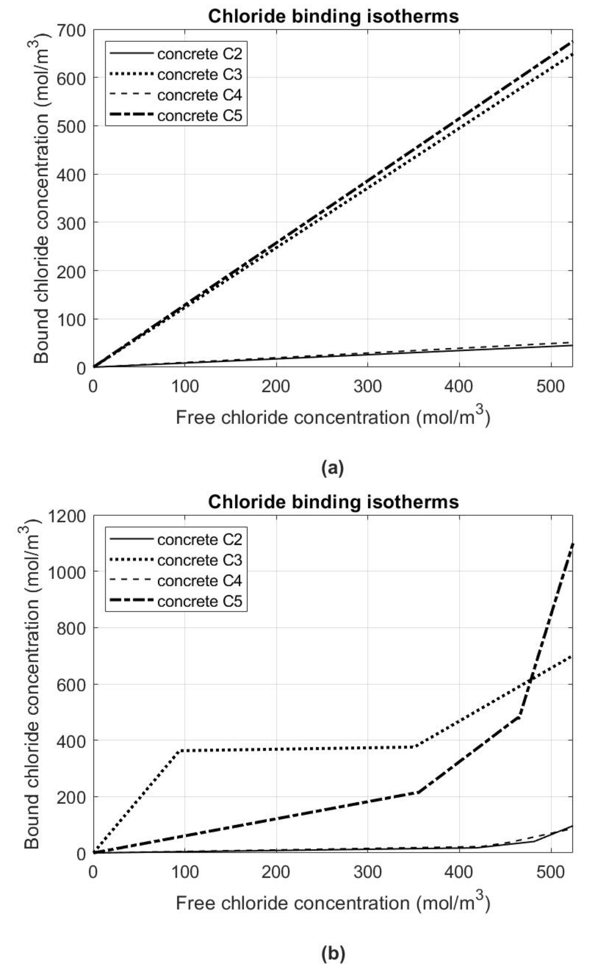
Figure 4 shows the determined courses of chloride binding isotherms in the case of data from Table 5 for the linear approximation (Figure 4a) and data from Table 7 for the spline approximation (Figure 4b). For both descriptions of the problem, it can be clearly stated that concretes C3 and C5, in which the blast furnace and pozzolanic cements were used, have an order greater capacity to bind chlorides than concretes C2 and C4 with the ash and low-alkali normal early strength Portland cements, respectively.

It can also be concluded that for concretes C3 and C5, the concentration of bound chlorides in the concrete skeleton is comparable to the concentration of free chlorides in the pore liquid. Moreover, the description of isotherms by the spline function (Figure 4b) gives much more information on the “skin effect” in accordance with the assumptions made in Section 3. In all C2–C5 concretes for the last section of isotherms, i.e., for free chloride concentrations comparable to the maximum concentration, we can observe increased chloride binding compared to the first two sections of the isotherms. Due to the fact that it concerns the experimental data after 6 months of the diffusion process under the constant boundary conditions of the first kind, its most intense part is at the same time located at the outer surface of the samples. It also indicates that there is much more hardened cement paste in this subsurface layer compared to the bulk parts of samples that it has a noticeable effect in binding chlorides. It is related to the apparent diffusion coefficient decrease in the subsurface layer compared to the effective one by about an order for concretes C2–C4 and by as much as two orders for C5 concrete (Table 7).

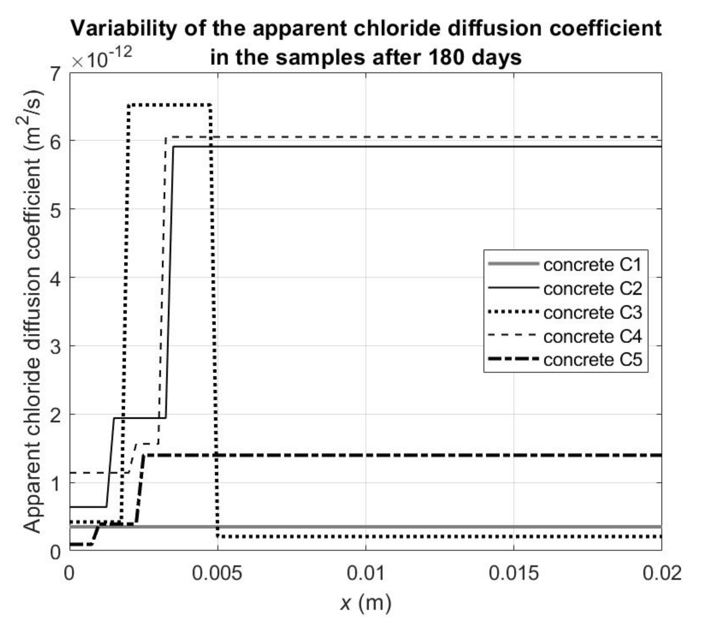
Figure 5 illustrates the changes in the apparent chloride diffusion coefficients depending on the depth of the samples after 180 days from the beginning of the chloride diffusion process, which enables a more accurate estimation of the extent of the “skin effect”. At this moment, we can distinguish three zones with different advancement of the chloride binding process:

(1)

The first zone is located to a depth of approx. 1–2 mm from the outer surface of the samples. Apparent chloride diffusivity is significantly reduced compared to effective diffusivity. This is the result of a significantly increased proportion of the cement matrix in relation to the aggregate compared to the bulk part of concrete, and thus increased chloride binding.

(2)

The second zone is located at a depth of about from 1–2 mm to 3–5 mm from the outer surface of the samples. In this zone, the apparent chloride diffusivity values of concretes C2, C4, and C5 are intermediate ones between the first and third zones, which may be the result of an increased content of cement paste compared to the third zone identical to the bulk part of concrete. However, the content of the cement paste is already smaller in the second zone compared to the first one. In the case of concrete C3, in its second zone, the value of apparent diffusivity is only twice lower than the effective one (see Table 7), which may indicate that this is a zone with a structure comparable to the inner third zone and the process of chloride binding in this layer is much closer to completion after 180 days of the experiment.

(3)

The third zone is located at a depth of more than 3–5 mm from the outer surface. The values of apparent chloride diffusivity in this zone characterize the bulk part of concrete not disturbed by the occurrence of the “skin effect” and when the chloride binding process is just beginning.

As a result of the calculations made, it can also be concluded that the “skin effect” resulting from the changed concrete structure near the external surfaces (not in contact with the walls of the forms as in the experiment) occurs with the greatest intensity up to a depth of approx. 1–2 mm, however the cement matrix must also be capable of absorbing chloride ions, thereby significantly reducing the apparent diffusion coefficient. It should be emphasized at this point that the “skin effect” understood in this way under the conditions of immersing the concrete in a solution with chlorides can only last until the outer layer is fully saturated with them. The “skin effect” associated with the reduction in the apparent diffusivity of chlorides is also noticeable at a depth of about 1–2 mm to 3 mm in the case of concretes C2, C4, and C5, but to a lesser extent.

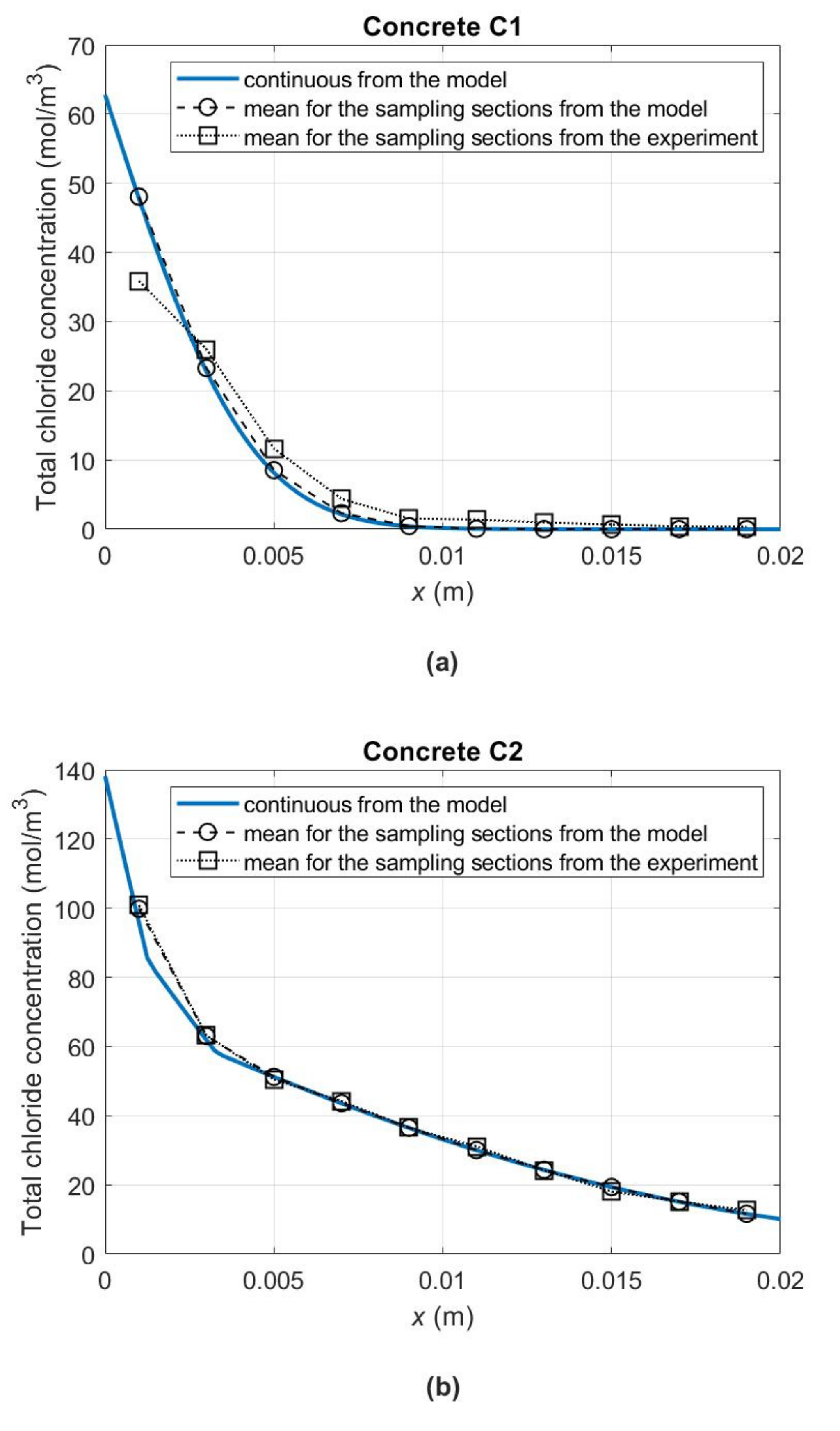
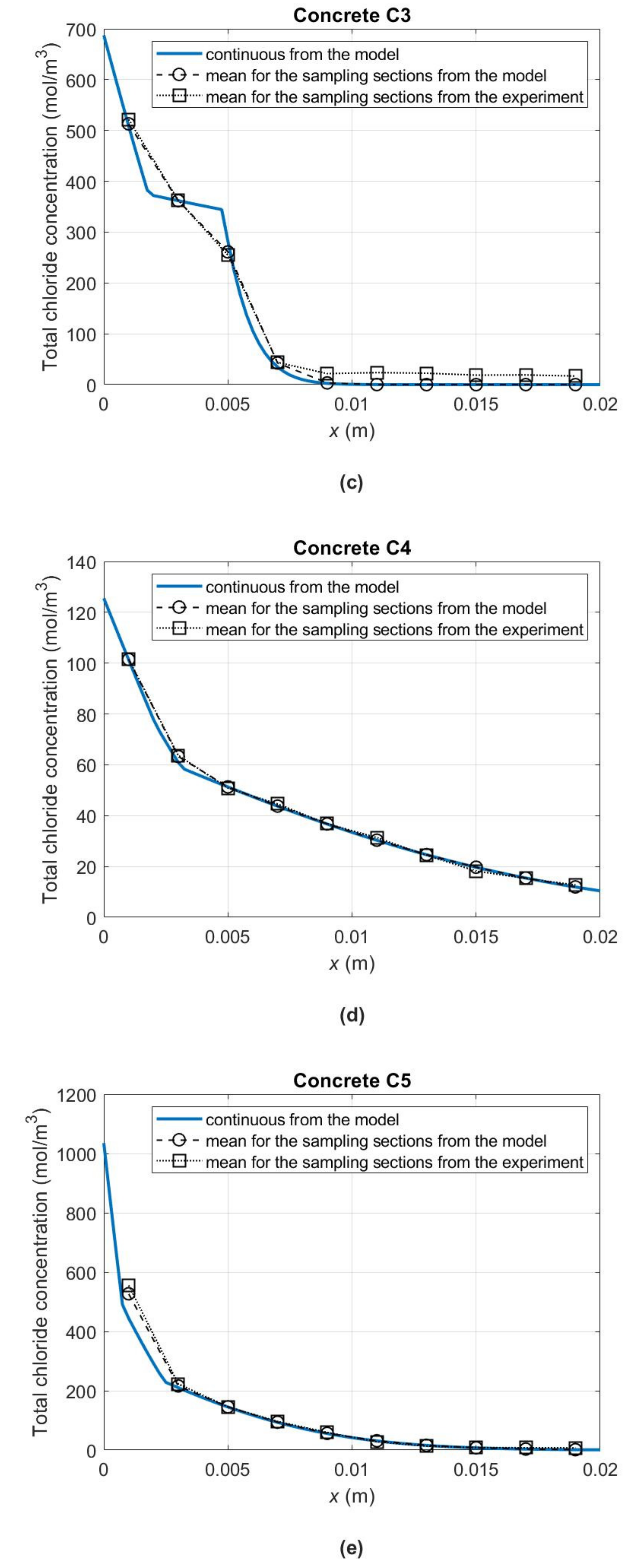
Figure 6 shows the concentration profiles of total chloride ions ($C_{\mathrm{t}}$) in the concrete samples up to a depth of 2 cm at 180 days from the start of the diffusion process. To obtain them for concrete C1, material parameters from Table 5 were used, and for concretes C2–C5 from Table 7. Importantly, also in the diagrams of Figure 6b–e, the occurrence of the “skin effect” in the case of C2–C5 concretes can be noticed. As a result of changes in the slopes of chloride binding isotherms in the individual concentration subintervals (Figure 4b) and the related changes in the apparent diffusivity of chlorides in individual sample zones (see Figure 5 with the zones distinguished after 180 days of the experiment), we also observe discontinuity points in the slopes of the curves describing the distribution of total chloride concentrations. In Figure 6, for illustrative purposes, the 180-day average concentrations of total chlorides in the samples’ successive layers with a thickness of 2 mm, determined experimentally (${\overline{C}}_{\mathrm{t}\exp }$) and calculated according to the model (${\overline{C}}_{\mathrm{t}\mathrm{model}}$), were also plotted. As a result of the comparison, a satisfactory agreement between the measurement and model data can be noticed.

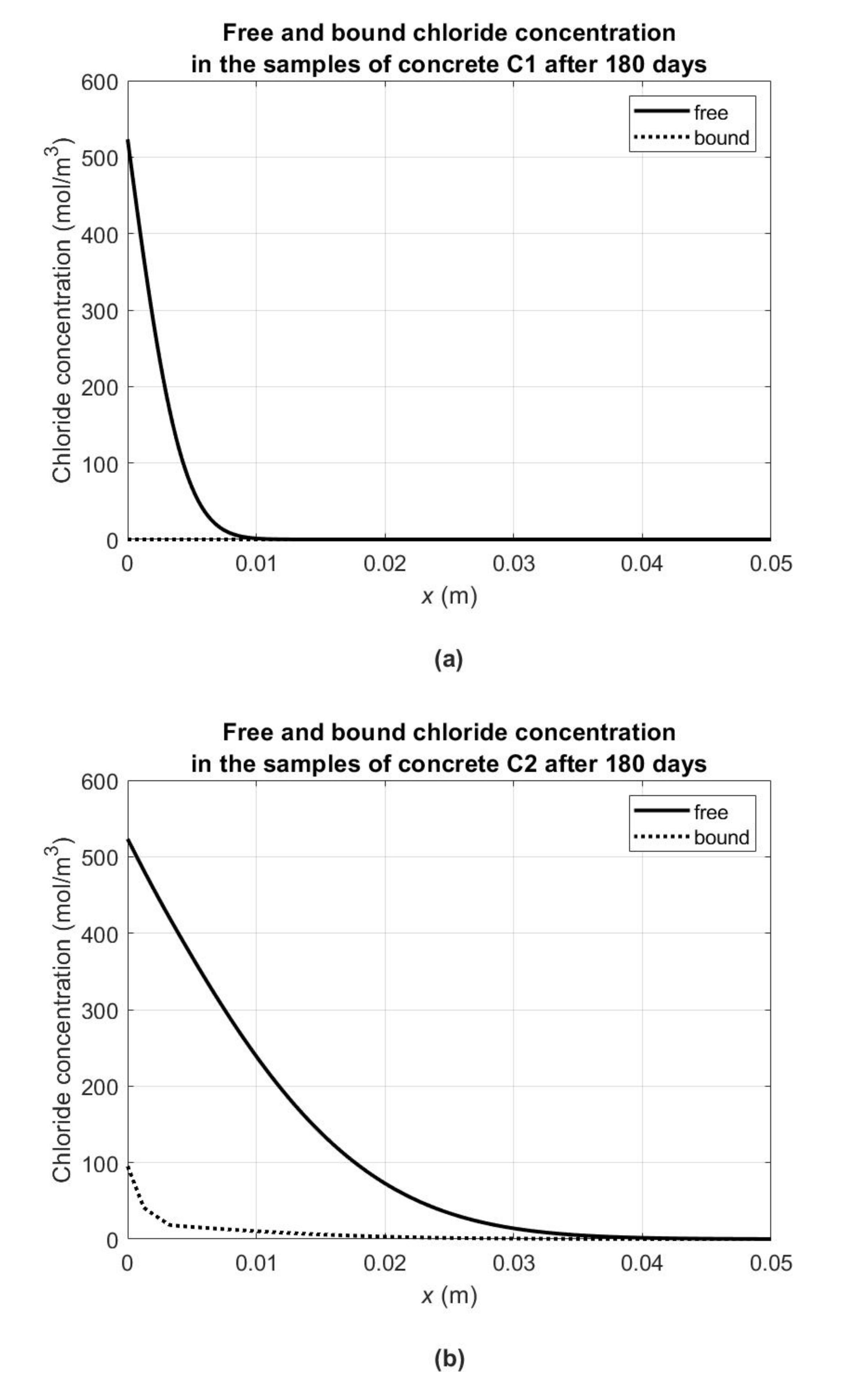
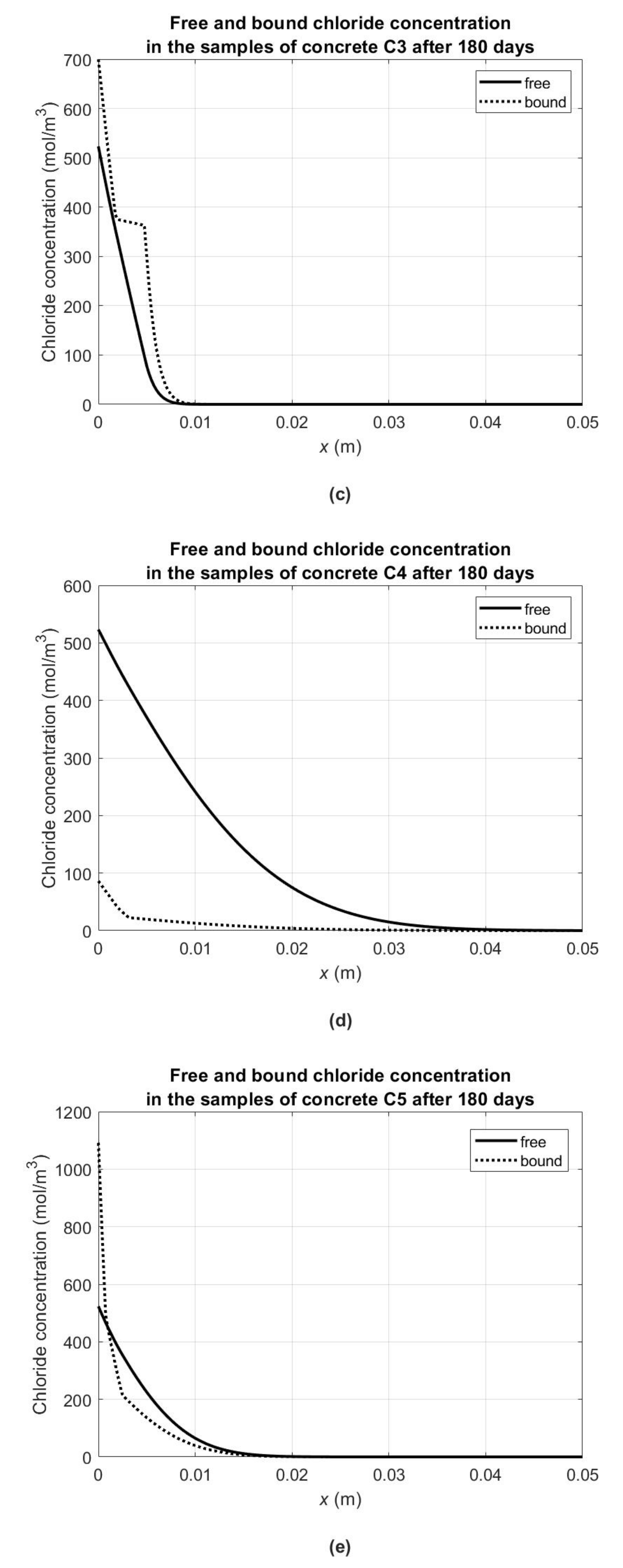
In order to illustrate the chloride binding capacity of the tested concretes, comparative graphs of bound ($C_{\mathrm{b}}$) and free ($C_{\mathrm{f}}$) chloride concentrations at 180 days from the start of the diffusion process are presented in Figure 7. Similarly to the previous figure, in order to obtain them, the material parameters from Table 5 for concrete C1 and from Table 7 for concretes C2–C5 were used. As mentioned, in the case of concrete C1 (with high early strength Portland cement), no chloride binding for the given experimental conditions was found (Figure 7a). For the remaining concretes, the chloride binding process was most intense in concretes C5 (with pozzolanic cement—Figure 7e) and C3 (with blast furnace cement—Figure 7c), where the chloride concentration exceeded the concentration of free chlorides in the subsurface layers. On the other hand, in the case of concretes C2 (with ash Portland cement—Figure 7b) and C4 (with low-alkali normal early strength Portland cement—Figure 7d), the concentration of bound chlorides in the subsurface layers is approximately five times lower than the free ones. At the same time, it should be noted that in accordance with the assumptions of the model (see Section 3), the concentration of free chlorides describes their concentration in the pore liquid, and the concentration of bound chlorides describes their average concentration in the solid concrete phase.

5. Conclusions

The most important results achieved in the work can be formulated in the following points:

(1)

Using a spline function to a description of chloride binding isotherm for 180-day diffusion experiments enables an assessment of the “skin effect” in terms of depth of its occurrence and change in apparent chloride diffusivity, which results from a different concrete composition and structure and thus different chloride binding properties in subsurface layers compared to a bulk part of material.

(2)

From five types of concretes tested in the study, concrete C1 containing high early strength Portland cement (CEM I 42.5 R) showed the best protective properties in terms of chloride corrosion due to the lowest effective diffusion coefficient of order of 10⁻¹³ m²/s (Table 5). There was no simultaneous binding of chlorides during the 180 days of diffusion.

(3)

The remaining C2–C5 concretes were characterized by one to two orders of higher effective diffusion coefficient than concrete C1, but at the same time they demonstrated chloride binding which led to a reduction in the apparent diffusion coefficients in the near-surface layers also to the value of order of 10⁻¹³–10⁻¹⁴ m²/s for concretes C2, C3, and C5, and for C4 to a value of order of 10⁻¹² m²/s (Table 7).

(4)

The highest chloride binding occurred in concrete C3 with blast furnace cement (CEM III/A 42.5 N-LH/HSR/NA) and concrete C5 with pozzolanic cement (CEM IV/B(V) 32.5 R-LH/NA). The concentrations of bound chlorides in the solid phase could maximally reach values comparable to the concentration of free chlorides in the pore liquid. Less chloride binding occurred in concrete C4 with low-alkali normal early strength Portland cement (CEM I 42.5 N-SR3/NA) and concrete C2 with ash Portland cement (CEM II/BV 32.5 R) where the concentration of bound chlorides in the solid phase could only be about five times lower than the concentration of free chlorides in the pore liquid.

(5)

Taking into account the chloride binding properties of concretes C2–C5, it can be stated that they also showed protective properties against chloride corrosion in the near-surface layers. However, in the case of concretes C2–C5 and in particular concretes C3 and C5, it should be remembered that after the initiation of chloride corrosion of the steel reinforcement, consumption of free chlorides in corrosive reactions and reduction of their concentration in the porous liquid may be related to re-releasing the bound chlorides and further “driving” the corrosion process [34].

(6)

The authors expect that thanks to the proposed mathematical model and calculation procedures, it is possible to assess the “skin effect” for different types of concrete, chloride compounds ingressing into it, and the methods of its curing and surface finishing what is important in view of the fact that such an effect basically always occurs due to executive and environmental factors in practical conditions. At the present stage of the research, the precise quantitative results presented in the article can be used to assess the chloride corrosion resistance of ordinary concrete only treated with solution of sodium chloride, with similar recipes using the same type of cement, aggregate, and methods of curing and finishing. For concretes with other recipes, qualitatively (not quantitatively) similar results can be expected, if the same types of cements, aggregates, and curing and finishing methods are used, and if sodium chloride solution is a source of chloride ions. It should be emphasized that due to the complexity of the problem, an unequivocal confirmation and evaluation of the protective properties in case of concrete with a given recipe, curing and surface finishing method, and source of chloride ions are only possible when the entire procedure proposed in the article is carried out anew.

(7)

The presented research requires continuation in the context of conclusion no. 6. This is the reason the authors want to first investigate, in accordance with the proposed assessment method, how the concrete surface finishing may change its protective properties against the chloride corrosion in reinforced concrete structures. From a practical point of view, the conclusions obtained this way may be used to form interesting technical recommendations for designers and contractors of concrete structures particularly exposed to chloride ingress.