An Artificial Neural Network-Based Equation for Predicting the Remaining Strength of Mid-to-High Strength Pipelines with a Single Corrosion Defect

Abstract

Numerical methods such as finite element analysis (FEA) can accurately predict remaining strength, with strong correlation with actual burst tests. However, parametric studies with FEA are time and computationally intensive. Alternatively, an artificial neural network-based equation can be used. In this work, an equation for predicting the remaining strength of mid-to-high strength pipelines (API 5L X52, X65, and X80) with a single corrosion defect subjected to combined loadings of internal pressure and longitudinal compressive stress was derived from an ANN model trained based on FEA results. For FEA, the pipe was assumed to be isotropic and homogenous, and the effects of temperature on the pipe failure pressure were not considered. The error of remaining strength predictions, based on the equation, ranged from −6.33% to 2.39% when compared to an unseen FEA dataset, with a correlation value (R²) of 0.9975. A parametric study was subsequently performed using the equation to determine the effects of material property, defect depth, defect length, and longitudinal compressive stress on the remaining strength of pipelines with a single corrosion defect. Defect depth reduced the failure pressure by more than 65% on average, longitudinal compressive stress by more than 20% on average, and defect length by more than 21% on average.

1. Introduction

Pipelines play a critical role in the continuous supply of hydrocarbons from one point to another. They are often subject to harsh and corrosive environments, with corrosion potentially causing pipeline failure and resulting in environmental damage and economic losses. Corrosion reduces pipe thickness, thus weakening pipeline strength, and corrosion defects in pipelines affect cylindrical symmetry, which affects structural efficacy of resisting stress [1]. Stresses from internal pressure and external load often concentrate at the corrosion region, further reducing the remaining strength of a corroded pipeline [2].

Maintaining the integrity of pipelines requires routine inspection and remaining strength assessments. Assessment standards such as ASME B31G, Modified B31G, RSTRENG Effective Area, PCORRC, and DNV RP-F101 are widely used to determine the remaining strength of corroded pipelines. However, they are mostly applicable for corroded pipelines with single defects only subjected to internal pressure. Of all the established corrosion assessment standards, DNV RP-F101 is the most comprehensive, as it can assess the remaining strength of a corroded pipeline with single defect corrosion subjected to internal pressure and longitudinal compressive stress. However, the remaining strength assessment using DNV RP-F101 is conservative due to the assumptions and simplifications made for their safety factors [3]. Pipelines are usually pressurised to transport hydrocarbons, and they experience hoop stress due to internal pressure uniformly acting outward in a circumferential direction. External loadings such as longitudinal stresses are often caused by geological movement and thermal stress [4]. Longitudinal compressive stress often causes buckling and wrinkling failure, thus reducing the remaining strength of corroded pipelines when they are subjected to combined loadings [5,6,7]. A corroded pipeline will fail below the remaining strength predicted by DNV when the combined stresses due to internal pressure and external loads exceed ultimate tensile strength of the pipeline.

Numerous experimental and numerical studies have been carried out to understand the failure of pipelines subjected to the combined loadings of internal pressure and longitudinal stress. Bjørnøy et al. carried out full-scale burst tests on twelve API 5L X52 grade steel pipelines with artificially created corrosion defects as part of the development of DNV RP-F101 assessment standards for corroded pipelines [8]. Their work revealed significant effects of bending moment and axial compressive stress on the remaining strength of a pressurised corroded pipeline, especially for a pipeline with a deep corrosion defect. Bjørnøy et al.’s work was supported by findings from Chauhan et al.’s work on high strength pipelines and Halima and Sreekanta’s studies on corroded X46 steel pipelines [9,10].

However, burst tests are expensive and time consuming. Numerical methods such as the finite element method (FEM) are widely used to verify and validate the failure behaviour and remaining strength of corroded pipelines [11,12,13,14,15]. These methods are especially useful for parametric studies with varying corrosion geometries that would otherwise will be too costly to be experimentally carried out. They have proven to be better than the established standards to assess remaining strength of corroded pipeline [12].

However, parametric studies with numerical methods are time and computationally intensive. Alternatively, an artificial neural network (ANN) may be used to predict the remaining strength of corroded pipes with single corrosion defects and interacting corrosion defects based on a data-driven machine learning framework, with the datasets derived from FEA results and full-scale burst tests. Some of these ANN models are described in

Table 1. ANN based on FEA dataset to predict the failure pressure of corroded pipelines.

Scheme	Corrosion Type	Loads	Material	ANN Algorithm
Silva et al. (2007) [16]	Interacting defects (longitudinally and circumferentially aligned)	Internal pressure	X52	Feedforward neural network
Xu et al. (2017) [17]	Single and interacting defects (longitudinally and circumferentially aligned)	Internal pressure	X80	Feedforward neural network
Lu and Liang (2021) [18]	Single defects	Internal pressure and axial compressive load	X65, X70, X80	Not specified

.

However, these studies have not provided closed-form equations, such as the ANN-based closed-form equation to predict the load-carrying capacity of locally corroded steel plate girder ends by Tohidi and Sharifi (2016) [19]. The authors of this paper propose an ANN-based equation to predict the failure pressure of a mid-to-high strength pipeline with a single corrosion defect subject to combined loadings of internal pressure and longitudinal compressive stress.

2. Materials and Methods

FEM was used to determine the remaining strength of middle-to-high strength pipelines, namely API 5L X52, API 5L X65, and API 5L X80 grade pipelines, subjected to combined loadings of internal pressure and longitudinal compressive stress; the results of these evaluations were then used to train an ANN model. The datasets for X52 and X80 were obtained from previous studies [20,21], while the dataset for X65 was generated in this study. The FEM results of the X65 grade pipeline’s remaining strength was validated with results from burst tests. The FEA datasets of the X52, X65, and X80 grade pipelines were then used to train an ANN model. The weights and biases of the ANN model were used to as the basis for the artificial neural network-based equation.

3. Methodology

This section is divided by subheadings. It provides a concise and precise description of the experimental results, their interpretation, and the experimental conclusions.

3.1. Finite Element Method for X65 Pipeline

ANSYS (16.1) Mechanical APDL was used for the FEM. The considered material was an API 5L X65 grade steel pipeline, and the pipe model had an external diameter (D_e) of 300 mm, a wall thickness (t) of 10 mm, and a pipe length (L) of 2000 mm. A quarter of the symmetrical pipe was modelled with a corrosion defect to reduce the needed computational resources. Figure 1 shows the dimension of the quarter pipe model.

The corrosion defect was rectangular with varying defect depth, length, and width. The pipe was subjected to external longitudinal compressive stress. The range of parameters selected for this study is shown in

Table 2. Geometric parameters for corrosion defect and load applied to the corroded X65 pipeline.

Parameters	Range
Defect Depth, d/t	0.2, 0.4, 0.5, 0.6, 0.8
Defect Length, l/D	0.2, 0.4, 0.8, 1.2, 1.8
Defect Width, w/t	2, 6, 10, 14, 18
$$\begin{gathered} \mathrm{Longitudinal}\mathrm{Compressive}\mathrm{Stress}, \\ {\sigma }_c/{\sigma }_y \end{gathered}$$	0.2, 0.4, 0.5, 0.6, 0.8, 1.0

.

A pipe end cap was modelled for the application of longitudinal compressive stress to ensure more accurate FEA results [13]. Figure 2 shows the internal pressure applied on the internal surfaces, while longitudinal compressive stress was applied on the surface of the end cap. The loads were incrementally applied using timesteps through ramped loading in ANSYS. Longitudinal compressive stress was incrementally applied in the first timestep. Internal pressure was then incrementally applied in the second timestep while maintaining the load in the first timestep.

The pipe body was brick-meshed with a SOLID185 element, and the pipe end cap was free-meshed with a SOLID186 element. The corrosion defect depth was modelled with three layers of element, and the thickness of the pipe was modelled with six layers of element for more accurate FEA [22]. To prevent unwanted motion when longitudinal compressive stress was applied, the model was constrained in three nodes near the end cap, as denoted by the triangle symbol in Figure 3 [20,23,24]. Preliminary analysis showed negligible differences between the number of constrained nodes and their position (in the region at the end of the pipe model), with solution convergence. The density of element for the pipe model was distributed based on the region of interest in this study. The density at corrosion defect was the highest, and the element density gradually decreased away from the corrosion defect, as shown in Figure 3.

The true stress–strain curve of an API 5L X65 pipeline, as shown in Figure 4, was used to define its material property in ANSYS. Static, non-linear, structural analysis (Newton–Raphson) was used in the FEM to account for the non-linearity of the material.

The pipe end cap was considered to be rigid body to prevent deformation when longitudinal compressive stress was applied. A high stiffness material property was used for the pipe end cap.

Table 3. Mechanical properties of the pipe model.

	Pipe Body—API 5L X65 (SOLID185)	Pipe End Cap—Rigid Body (SOLID186)
Modulus of Elasticity, E	210 GPa	210 TPa
Poisson’s ratio, v	0.3	0.3
$\mathrm{Yield}\mathrm{Strength},{\sigma }_y$	464 MPa	-
$\mathrm{Ultimate}\mathrm{tensile}\mathrm{strength},{\sigma }_u$	563 MPa	-
$\mathrm{True}\mathrm{ultimate}\mathrm{tensile}\mathrm{strength},{\sigma }_u*$	629 MPa	-

lists the mechanical properties of the pipe body and end cap.

The failure criterion adopted in this study was based on true ultimate tensile strength (UTS) of API 5L X65, as the criterion provides more accurate results [17,20]. Pipe failure occurs when the von Mises stress reaches the reference stress (UTS) across the entire wall thickness, resulting in plastic collapse of the pipe.

3.2. Validation of Finite Element Method

The FEM results were validated with results from full-scale burst tests by Kim et al. and Bjørnøy et al. [8,26]. Kim et al. performed burst tests on an API 5L X65 pipeline with a single corrosion defect subjected to internal pressure. Their pipe specimens had an outer diameter of 762 mm, a wall thickness of 17.5 mm, and a pipe length of 2.3 m. Kim et al.’s burst test results were used to validate the material property of the API 5L X65 pipeline used in this study. Bjørnøy et al. carried out full-scale burst tests on an API 5L X52 pipeline with a single corrosion defect subjected to internal pressure and longitudinal compressive stress. Their pipe specimens had an outer diameter of 324 mm, a wall thickness of 10.3 mm, and a pipe length of 1.0 m. Bjørnøy et al.’s burst test results were used to validate the boundary conditions for the internal pressure and longitudinal compressive stress considered in this study.

Table 4. Validation of FEM results against burst test for pipes only subjected to internal pressure and combined loadings of internal pressure and longitudinal compressive stress.

Specimen	Failure Pressure from Burst Tests (MPa)	Failure Pressure Predicted in FEM (MPa)	Absolute Percentage Difference (%)
LD	19.8	20.1	1.50
LF	15.0	15.5	3.67
Test 5	28.6	29.2	2.10
Test 6	28.7	29.6	3.14

shows the validation results. The difference between the failure pressure predicted by the FEM and burst test was relatively small, with a maximum difference of 3.67%. Therefore, the FEM employed in this study was accurate.

3.3. Artificial Neural Network

An artificial neural network (ANN) is a machine learning technique suitable for supervised learning. It can be used to solve regression problems because of its ability to map complex relationship in a nonlinear dataset. In this study, a feedforward neural network (FFNN) was used. The network comprised an input layer, hidden layer(s), and an output layer. The network was trained with the FEA results of the X52, X65 and X80 pipelines with a single corrosion defect subjected to internal pressure and longitudinal compressive stress. In the ANN, the true UTS of the pipes, corrosion defect parameters, and longitudinal compressive stress were used as inputs, and their corresponding failure pressure was the target output. The inputs and outputs were normalised to prevent inputs with large values from dominating other inputs. The X52, X65, and X80 FEA results were randomly divided into a training set (70%), a validation set (15%), and a test set (15%). The validation and test sets were used to prevent overfitting. The Levenberg–Marquardt (LM) backpropagation algorithm was used as the learning algorithm to train the ANN model. The LM backpropagation algorithm is more efficient than other learning algorithms due to its second-order convergence rate. It converges faster in fewer epochs [27]. The architecture of the neural network was reconfigured through trial and error in order to prevent overtraining and improve prediction accuracy. Hyperparameters such as the number of hidden neurons and the number of hidden layers were tuned so that the mean squared error, MSE < 1 × 10⁻⁵. The ANN development framework is shown in Figure 5.

The training process of the FFNN is further described in Figure 6. The weight and biases of the link between neurons were randomly initialised instead of the default zero value. The normalised inputs were moved through weighted links between the input neurons and hidden neurons. They were then calculated based on the activation function of the neurons, as well as their weights and biases. The performance of the neural network was measured using a cost function. The error between the predicted output and expected output was calculated based on the cost function. The weights and biases of the neurons were subsequently updated to minimise errors.

The performance of the ANN was evaluated through the coefficient of determination (R²) in Equation (1), mean squared error (MSE) in Equation (2), and mean absolute error (MAE) in Equation (3).

$$R^2={\left(\frac{{{\displaystyle \sum }}_{i=1}^N\left(y_i-{\overline{y}}_i\right)\left({\widehat{y}}_i-{\overline{\widehat{y}}}_i\right)}{\sqrt{{{\displaystyle \sum }}_{i=1}^N{\left(y_i-{\overline{y}}_i\right)}^2{{\displaystyle \sum }}_{i=1}^N{\left({\widehat{y}}_i-{\overline{\widehat{y}}}_i\right)}^2}}\right)}^2$$

(1)

$$\mathrm{MSE}=\frac{1}{N}{\displaystyle \sum }_{i=1}^N{\left({\widehat{y}}_i-y_i\right)}^2$$

(2)

$$\mathrm{MAE}=\frac{1}{N}{\displaystyle \sum }_{i=1}^N\left|y_i-{\widehat{y}}_i\right|$$

(3)

where ${\widehat{y}}_i$ and $y_i$ are the actual and predicted output values for the ith output, respectively; ${\overline{\widehat{y}}}_i$ and ${\overline{y}}_i$ are the average of actual and predicted output, respectively; and N is the number of samples. R² or the squared correlation coefficient is the evaluation of goodness-of-fit for the predicted value against actual value, where an R² value of 1.00 corresponds to a perfect fit. The MSE is the sum of squared difference between the predictions and actual values. The MAE is the mean absolute error between predictions and actual values, which measures the accuracy of the predictions.

4. Results

4.1. Finite Element Analysis of API 5L X65 Pipeline with Single Corrosion Defect

To determine the effect of defect geometry and the load applied on the remaining strength of a corroded API 5L X65 pipeline with single corrosion defect, the defect parameters and external load were varied one factor at a time. The parameters were the defect depth d/t, defect length l/D, defect width w/t, and longitudinal compressive stress ${\sigma }_c/{\sigma }_y$. The FEA results were normalised and expressed as the ratio of the estimated failure pressure to the theoretical failure pressure of an intact pipe, $P_f/P_i$. Using Equation (4), the failure pressure of an intact pipe was calculated as 44.93 MPa. Equation (4) is the hoop stress equation based on true ultimate tensile strength (UTS) as the failure criterion:

$${\sigma }_{UTS\ast }=\frac{P_i{r}_i}{t}$$

(4)

where ${\sigma }_{UTS\ast }$ is the true UTS of API 5L X65, t is the thickness of the pipe, and $r_i$ is the radius of inner pipe.

Table 5. FEA of corroded X65 pipeline with single corrosion defect subjected to internal pressure and longitudinal compressive stress.

Defect Parameters			External Load	Normalised Failure Pressure	Defect Parameters			External Load	Normalised Failure Pressure
d/t	l/D	w/t	${\mathit{\sigma }}_{\mathit{c}}/{\mathit{\sigma }}_{\mathit{y}}$		d/t	l/D	w/t	${\mathit{\sigma }}_{\mathit{c}}/{\mathit{\sigma }}_{\mathit{y}}$
0.2	0.8	10	-	0.82	0.5	0.8	6	0.5	0.57
0.4	0.8	10	-	0.68	0.5	0.8	14	0.5	0.54
0.5	0.8	10	-	0.59	0.5	0.8	18	0.5	0.53
0.6	0.8	10	-	0.49	0.5	0.8	10	0.2	0.58
0.8	0.8	10	-	0.28	0.5	0.8	10	0.4	0.57
0.5	0.2	10	-	0.77	0.5	0.8	10	0.6	0.53
0.5	0.4	10	-	0.68	0.5	0.8	10	0.7	0.46
0.5	1.2	10	-	0.55	0.5	0.8	10	0.8	0.37
0.5	1.8	10	-	0.53	0.5	0.8	10	0.9	0.2
0.5	0.8	2	-	0.57	0.5	0.8	10	1.0	0.17
0.5	0.8	6	-	0.60	0.2	0.8	10	0.7	0.54
0.5	0.8	14	-	0.58	0.4	0.8	10	0.7	0.52
0.5	0.8	18	-	0.57	0.6	0.8	10	0.7	0.40
0.2	0.8	10	0.5	0.75	0.8	0.8	10	0.7	0.22
0.4	0.8	10	0.5	0.64	0.5	0.2	10	0.7	0.56
0.5	0.8	10	0.5	0.56	0.5	0.4	10	0.7	0.50
0.6	0.8	10	0.5	0.46	0.5	1.2	10	0.7	0.46
0.8	0.8	10	0.5	0.26	0.5	1.8	10	0.7	0.45
0.5	0.2	10	0.5	0.69	0.5	0.8	2	0.7	0.47
0.5	0.4	10	0.5	0.62	0.5	0.8	6	0.7	0.47
0.5	1.2	10	0.5	0.53	0.5	0.8	14	0.7	0.45
0.5	1.8	10	0.5	0.52	0.5	0.8	18	0.7	0.45
0.5	0.8	2	0.5	0.56

details the results of the finite element analysis.

4.2. Development of an Artificial Neural Network-Based Equation

The FEA results of the corroded X65 pipe provided insights for suitable parameters and their range in the development of the ANN model. The parameter that had the most impact on failure pressure was found to be defect depth, followed by longitudinal compressive stress, defect length, and defect width. The average reduction rates in failure pressure due to defect depth, longitudinal compressive stress, and defect length were −0.54, −0.41, and −0.06, respectively. The effect of defect width was negligible, as its average rate of decrement in failure pressure was −0.002. Therefore, the defect width was fixed at 10 w/t in the FEA of X65 for the ANN training dataset. The FEA results for the ANN training dataset are tabulated in

Table 6. FEA results of corroded X65 pipeline for ANN training dataset.

d/t	l/D	${\mathit{\sigma }}_{\mathit{c}}\mathbf{/}{\mathit{\sigma }}_{\mathit{y}}$
		0.2	0.4	0.5	0.6	0.7
0.2	0.2	0.88	0.85	0.79	0.74	0.61
	0.4	0.85	0.82	0.77	0.70	0.59
	0.6	0.84	0.79	0.75	0.68	0.56
	0.8	0.83	0.78	0.74	0.66	0.54
	1.2	0.81	0.77	0.73	0.65	0.53
0.4	0.2	0.80	0.76	0.71	0.67	0.59
	0.4	0.75	0.71	0.68	0.62	0.54
	0.6	0.70	0.68	0.65	0.61	0.53
	0.8	0.68	0.66	0.64	0.60	0.52
	1.2	0.65	0.63	0.62	0.59	0.52
0.5	0.2	0.77	0.73	0.69	0.64	0.56
	0.4	0.67	0.65	0.62	0.58	0.50
	0.6	0.61	0.60	0.58	0.54	0.47
	0.8	0.58	0.57	0.56	0.53	0.46
	1.2	0.55	0.54	0.53	0.52	0.46
0.6	0.2	0.72	0.69	0.66	0.61	0.53
	0.4	0.59	0.57	0.55	0.52	0.45
	0.6	0.53	0.51	0.49	0.47	0.41
	0.8	0.49	0.47	0.46	0.45	0.40
	1.2	0.45	0.45	0.44	0.43	0.39
0.8	0.2	0.58	0.56	0.55	0.52	0.44
	0.4	0.39	0.37	0.36	0.34	0.28
	0.6	0.32	0.30	0.29	0.28	0.24
	0.8	0.28	0.27	0.26	0.25	0.22
	1.2	0.25	0.24	0.24	0.23	0.21

.

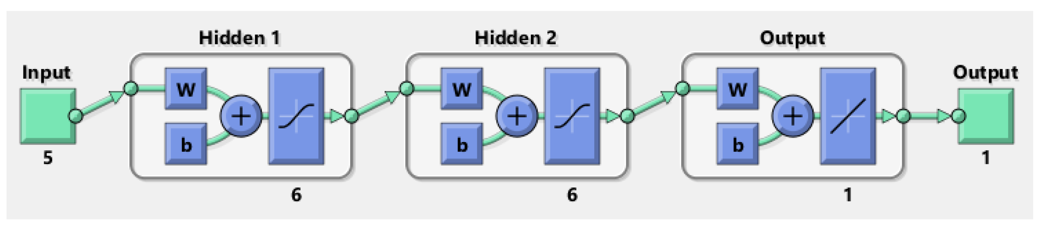
For the formulation of the empirical equation, 176 sets of X52 FEA results from the work of Arumugam et al. [19] and 81 sets of X80 FEA results from the work of Kumar et al. [20] were used to train the ANN [20,21], in addition to the FEA results of corroded X65 pipelines. The ANN model was developed using MathWorks MATLAB. The architecture of the ANN is illustrated in Figure 7.

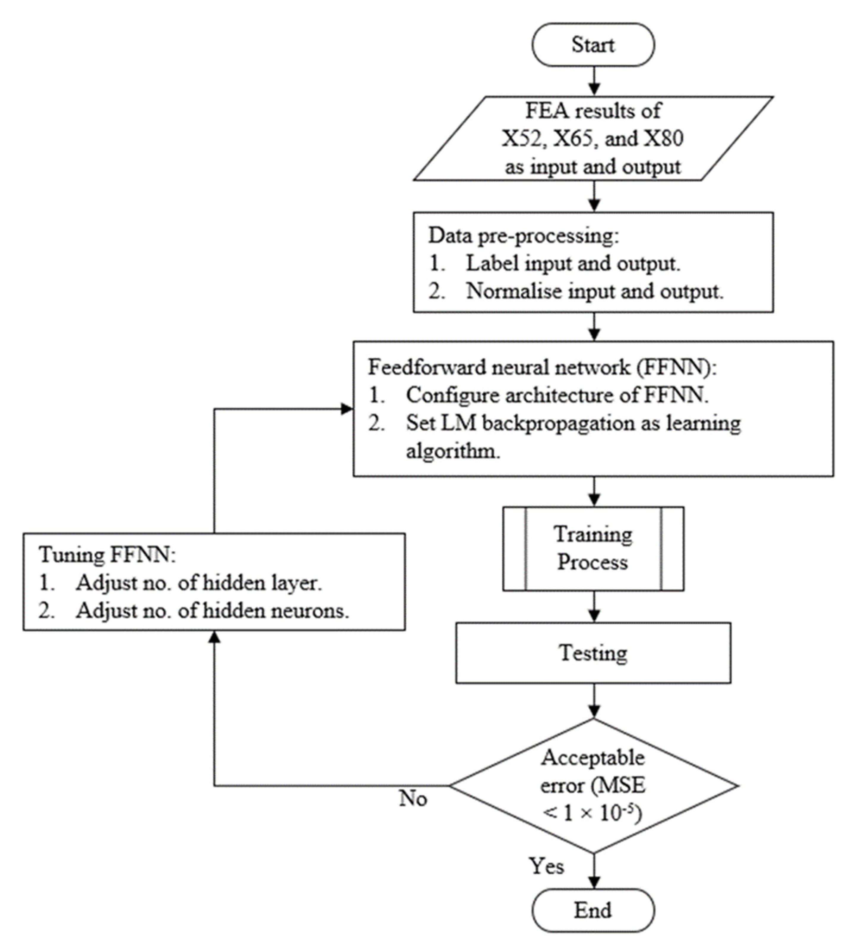
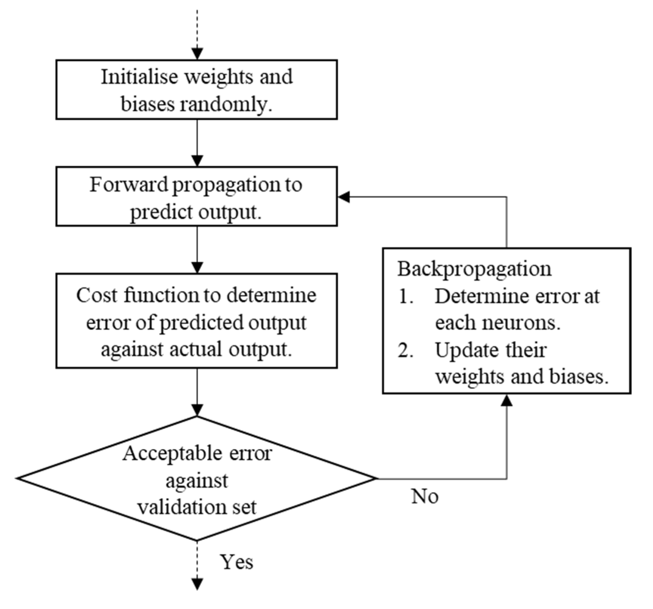
The ANN was based on a feedforward neural network (FFNN), with Levenberg–Marquardt backpropagation as its training algorithm. The inputs were the true UTS of the pipeline, normalised corrosion defect depth ($d/t$), normalised corrosion defect length ($l/D$), normalised corrosion defect width ($w/t$), and normalised axial compressive stress, ${\sigma }_c/{\sigma }_y$. The output was normalised failure pressure, $P_f/P_i$. The ANN had two hidden layers, with six hidden neurons in each layer. The number of hidden neurons was determined with trial and error to find the best performing configuration. The activation functions for the hidden layers were a hyperbolic tangent sigmoid transfer function and a linear transfer function for the output layer.

The input and output neurons were normalised, and the values of true UTS, $d/t$, $l/D$, $w/t$, ${\sigma }_c/{\sigma }_y$, and $P_f/P_i$ were set to be between the range from −1 to 1. Equation (5) was used to normalise the values to prevent inputs with large values from dominating other inputs.

$${\left(y\right)}_n=\frac{\left(y_{max}-y_{min}\right)\left(x-x_{min}\right) }{\left(x_{max}-x_{min}\right)}+y_{min}$$

(5)

where, $y$ is the normalisation value ranging from −1 to 1 and $x$ is denormalization value ranging according to its dataset.

After training the ANN, the weights and biases were adjusted for output predictions with the lowest errors. The connections between the input, output, hidden neurons, and their weights and biases were mathematically expressed, as shown in Equations (6)–(8).

$$\left[\begin{array}{c}{h}_{1,1}\\ h_{1,2}\\ h_{1,3}\\ h_{1,4}\\ h_{1,5}\\ h_{1,6}\end{array}\right]=\left[\begin{array}{ccccc}0.0290& -0.3112& 0.2976& -0.0501& 0.0044\\ -1.0552& 0.4619& 1.5820& 2.0369& 0.4190\\ -0.2548& 0.4752& -0.0036& 0.0093& -2.7614\\ 2.1350& 0.2060& 0.1957& -0.3347& 1.3200\\ -0.1720& 0.2548& 0.7511& -0.1147& -0.0504\\ 0.9064& 1.3703& 0.7865& -0.5071& -0.8183\end{array}\right]\left[\begin{array}{c}{\left(UTS\right)}_n\\ {\left(d/t\right)}_n\\ {\left(l/D\right)}_n\\ {\left(w/t\right)}_n\\ {\left({\sigma }_c/{\sigma }_y\right)}_n\end{array}\right]+\left[\begin{array}{c}0.4439\\ 2.8125\\ 2.1760\\ 0.6014\\ 0.0232\\ 1.8972\end{array}\right]$$

(6)

$$\left[\begin{array}{c}{h}_{2,1}\\ h_{2,2}\\ h_{2,3}\\ h_{2,4}\\ h_{2,5}\\ h_{2,6}\end{array}\right]=\left[\begin{array}{cccccc}0.8994& -0.5208& -0.1017& 1.6657& 0.5182& 0.8874\\ -1.1137& -0.4861& -1.3240& 0.2724& 0.7561& 1.0007\\ -1.4525& 0.7080& -0.4520& 0.6728& 1.4434& -0.7388\\ -0.9694& -1.0553& 1.5402& -1.8413& 1.0336& -1.9841\\ 0.2574& -0.2465& -0.6022& -0.4447& 0.6712& 0.8255\\ -2.5687& -0.0788& 0.2776& -0.4032& -2.4040& 0.4544\end{array}\right]\left[\begin{array}{c}a\left(h_{1,1}\right)\\ a\left(h_{1,2}\right)\\ a\left(h_{1,3}\right)\\ a\left(h_{1,4}\right)\\ a\left(h_{1,5}\right)\\ a\left(h_{1,6}\right)\end{array}\right]+\left[\begin{array}{c}-1.9775\\ 1.9334\\ 0.4981\\ 0.3314\\ -0.2197\\ -2.2699\end{array}\right]$$

(7)

$$\left[O_n\right]=f\left\{\left[\begin{array}{cccccc}0.7767& -1.4787& -0.8224& -0.5620& 1.2112& 1.3954\end{array}\right]\left[\begin{array}{c}a\left(h_{2,1}\right)\\ a\left(h_{2,2}\right)\\ a\left(h_{2,3}\right)\\ a\left(h_{2,4}\right)\\ a\left(h_{2,5}\right)\\ a\left(h_{2,6}\right)\end{array}\right]+\left[2.2849\right]\right\}$$

(8)

where, $a\left(x\right)$ is hyperbolic tangent sigmoid transfer function,

$$a\left(x\right)=\frac{2}{\left(1+e^{-2x}\right)-1} \mathrm{or}\tanh \left(x\right)$$

and $f\left(x\right)$ is linear transfer function,

$$f\left(x\right)=x$$

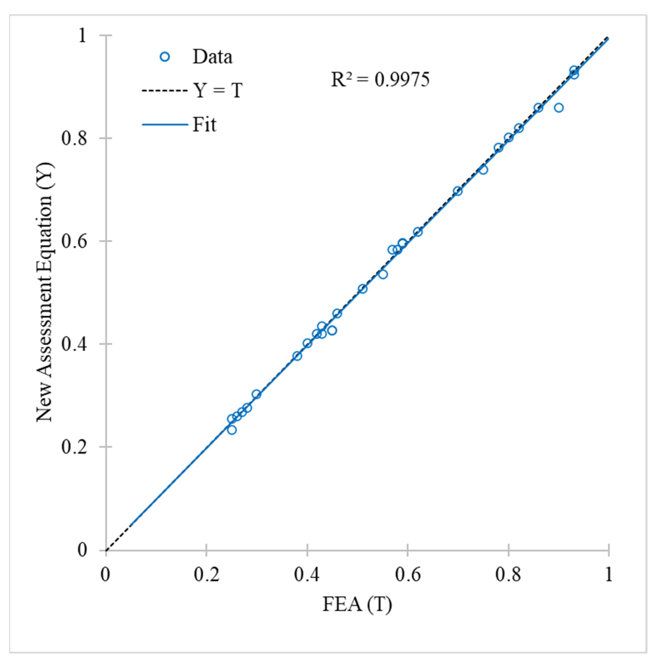
To ensure the reliability of the assessment equations, an unseen dataset was used to validate the method and determine its performance.

Table 7. Normalised failure pressure prediction using FEA and prediction based on the assessment equations of an unseen dataset.

Parameters				Normalised Failure Pressure		Difference
UTS	d/t	l/D	${\mathit{\sigma }}_{\mathit{c}}/{\mathit{\sigma }}_{\mathit{y}}$	FEA	New Equations	%
612.0	0.10	0.7	0.30	0.82	0.8194	−0.07
612.0	0.70	0.7	0.35	0.38	0.3766	−0.88
612.0	0.80	0.7	0.50	0.27	0.2680	−0.76
612.0	0.80	0.2	0.50	0.51	0.5078	−0.44
612.0	0.55	0.5	0.35	0.55	0.5352	−2.69
612.0	0.20	0.5	0.32	0.78	0.7814	0.18
612.0	0.70	0.5	0.25	0.43	0.4211	−2.07
612.0	0.35	0.7	0.60	0.57	0.5836	2.39
612.0	0.80	0.3	0.35	0.43	0.4355	1.29
612.0	0.10	0.3	0.60	0.75	0.7391	−1.46
629.0	0.70	0.5	0.25	0.46	0.4598	−0.05
629.0	0.10	0.3	0.30	0.90	0.8597	−4.48
629.0	0.45	1.1	0.45	0.59	0.5952	0.88
629.0	0.80	0.7	0.50	0.28	0.2767	−1.18
629.0	0.70	0.7	0.35	0.40	0.4015	0.39
629.0	0.80	0.3	0.60	0.42	0.4208	0.19
629.0	0.80	0.7	0.25	0.30	0.3037	1.24
629.0	0.80	1.1	0.50	0.25	0.2342	−6.33
629.0	0.30	0.3	0.30	0.80	0.8024	0.29
629.0	0.80	1.1	0.25	0.26	0.2595	−0.21
718.2	0.10	0.7	0.30	0.93	0.9320	0.22
718.2	0.30	0.3	0.30	0.86	0.8603	0.04
718.2	0.55	0.3	0.60	0.62	0.6188	−0.19
718.2	0.35	1.1	0.35	0.70	0.6970	−0.43
718.2	0.80	0.3	0.35	0.45	0.4264	−5.25
718.2	0.55	0.5	0.35	0.58	0.5831	0.53
718.2	0.80	0.7	0.60	0.25	0.2545	1.79
718.2	0.10	0.9	0.30	0.93	0.9246	−0.58
718.2	0.45	1.1	0.45	0.59	0.5965	1.10
718.2	0.70	0.5	0.25	0.45	0.4271	−5.09

presents the parameters and the FEA results of the 30 sets of unseen data. The table shows that the equations were accurate in their estimations of normalised failure pressure, with the percentage difference between FEA and the new equations ranging from −6.33% to 2.39% and a standard deviation of 2.12.

The R² value of the assessment equations when tested against an unseen dataset was 0.9975, which indicates good correlation, as shown in Figure 8. The assessment equation had an MSE of 0.000126 and an MAE of 0.00699.

4.3. Parametric Study Using the Artificial Neural Network-Based Equation

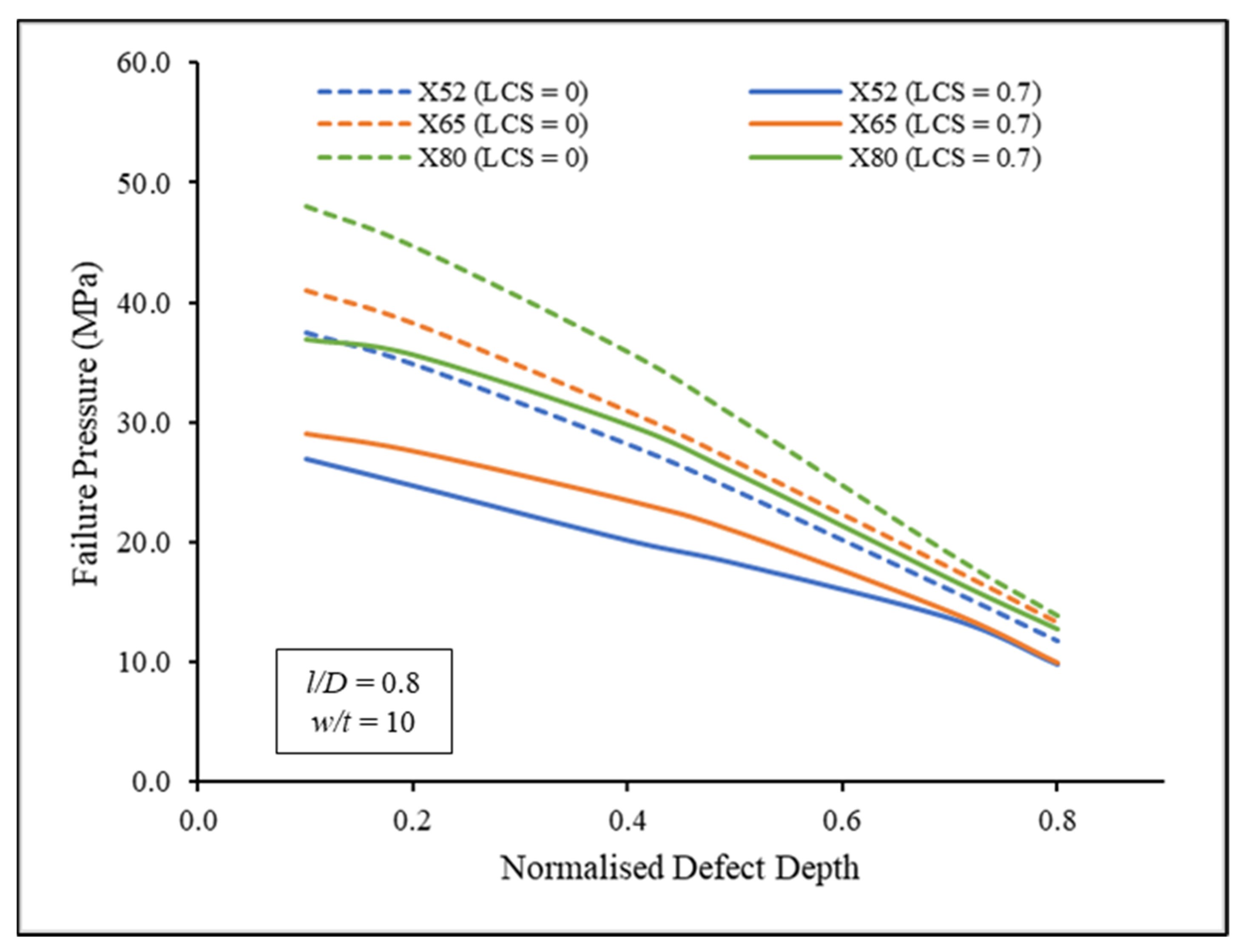
A parametric study was conducted to investigate the effects of material property, defect depth, defect length, and longitudinal compressive stress on the remaining strength of corroded pipelines with single corrosion defects. The middle-to-high strength pipelines considered in this study were X52, X65, and X80. Figure 9 shows the effect of defect depth on failure pressure for corroded pipelines with 0.0 and 0.7 ${\sigma }_c/{\sigma }_y$ longitudinal compressive stress when the defect length was fixed at 0.8 $l/D$ and defect width was fixed at 10 $w/t$. Figure 9 shows that the X80 trendline presented the highest failure pressure on average, followed by X65 and X52. The trendlines demonstrate the same behaviour, whereby the failure pressure of the corroded pipeline linearly decreases with an increase in defect depth, and the introduction of longitudinal compressive stress significantly reduced the failure pressure. For trendlines with no longitudinal compressive stress, the average failure pressure reduction rates per 0.1 $d/t$ of the X52, X65, and X80 pipelines were −8.51%, −8.87%, and −9.70%, respectively. For trendlines with 0.7 ${\sigma }_c/{\sigma }_y$, the average failure pressure reduction rates per 0.1 $d/t$ of the X52, X65, and X80 pipelines were −5.51%, −4.85%, and −6.92%, respectively. It can be observed that the average reduction rate for failure pressure was reduced when ${\sigma }_c/{\sigma }_y$ increased from 0.0 to 0.7. However, the failure pressure of the corroded pipe subjected 0.7 ${\sigma }_c/{\sigma }_y$ was still significantly lower than 0.0 ${\sigma }_c/{\sigma }_y$ (−23.99% on average). The trendlines of the same material type exhibited similar behaviour, whereby the failure pressure of 0.2 $d/t$ defects between 0.0 and 0.7 ${\sigma }_c/{\sigma }_y$ was reduced by almost half when the defect depth was 0.8 $d/t$. Similar trends were observed for defect lengths of 0.2, 0.4, 1.0, and 1.2 $l/D$.

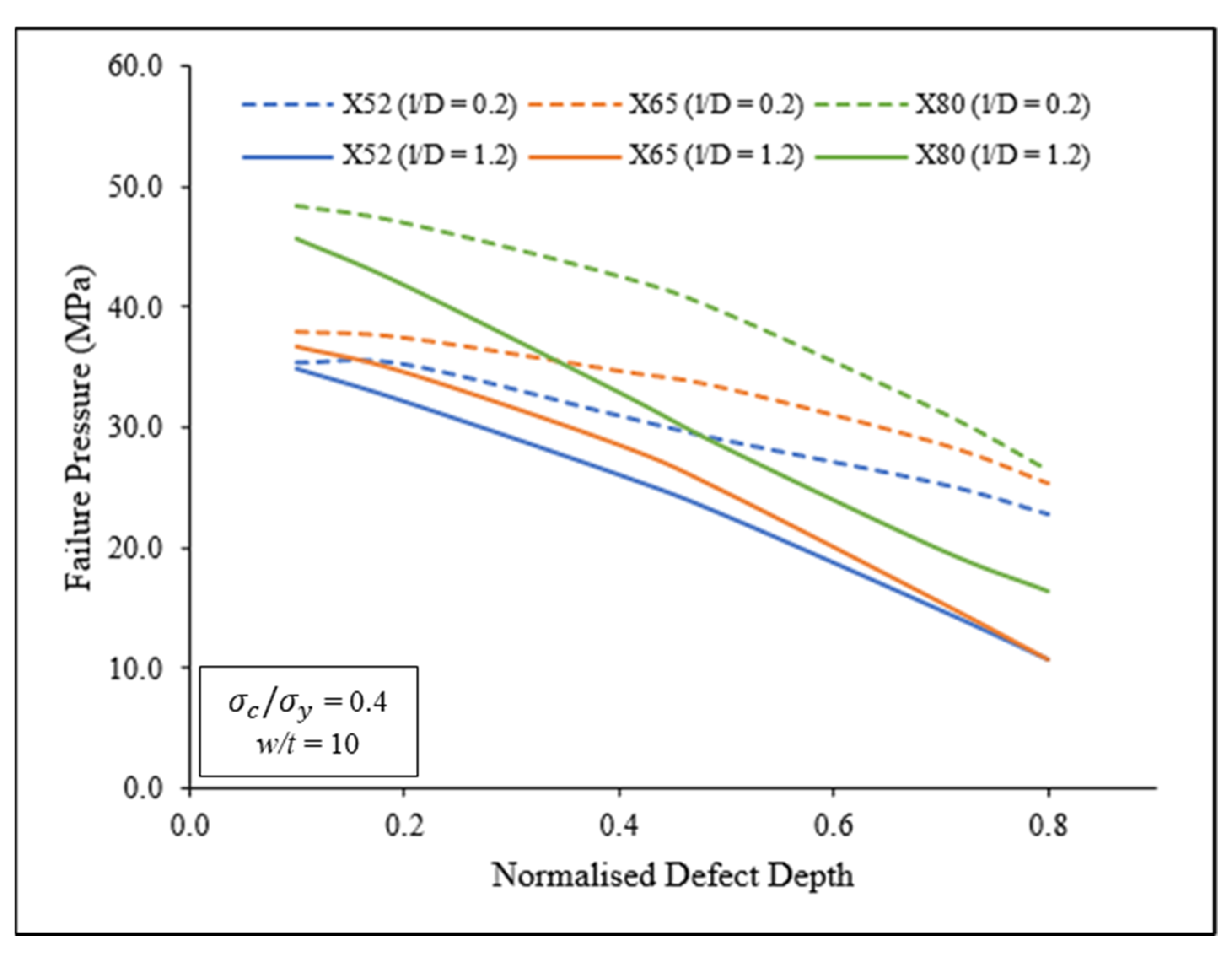
Figure 10 shows the effect of defect depth on the failure pressure of corroded pipelines with 0.2 and 1.2 $l/D$ defect lengths when the longitudinal compressive stress was 0.4 ${\sigma }_c/{\sigma }_y$. The trendlines of Figure 11 show that the failure pressure of the corroded pipelined linearly decreases with increasing defect depth, albeit not as steep as the trendlines in Figure 9. For trendlines with 0.2 $l/D$, the average failure pressure reduction rates per 0.1 $d/t$ of the X52, X65, and X80 pipelines were −4.29%, −3.94%, and −6.11%, respectively. For trendlines with 1.2 $l/D$, the average failure pressure reduction rates per 0.1 $d/t$ of the X52, X65, and X80 pipelines were −7.93%, 8.38%, and −8.33%, respectively. A comparison of shallow and deep corrosion defects showed that the average failure pressure reduction rate increased when $l/D$ increased from 0.2 to 1.2. This shows that increasing defect length of deeper corrosion defects could lower the failure pressure of a corroded pipeline (by −21.94% on average). Similar trends were also observed for longitudinal compressive stresses of 0.0, 0.2, 0.5, and 0.7 ${\sigma }_c/{\sigma }_y$.

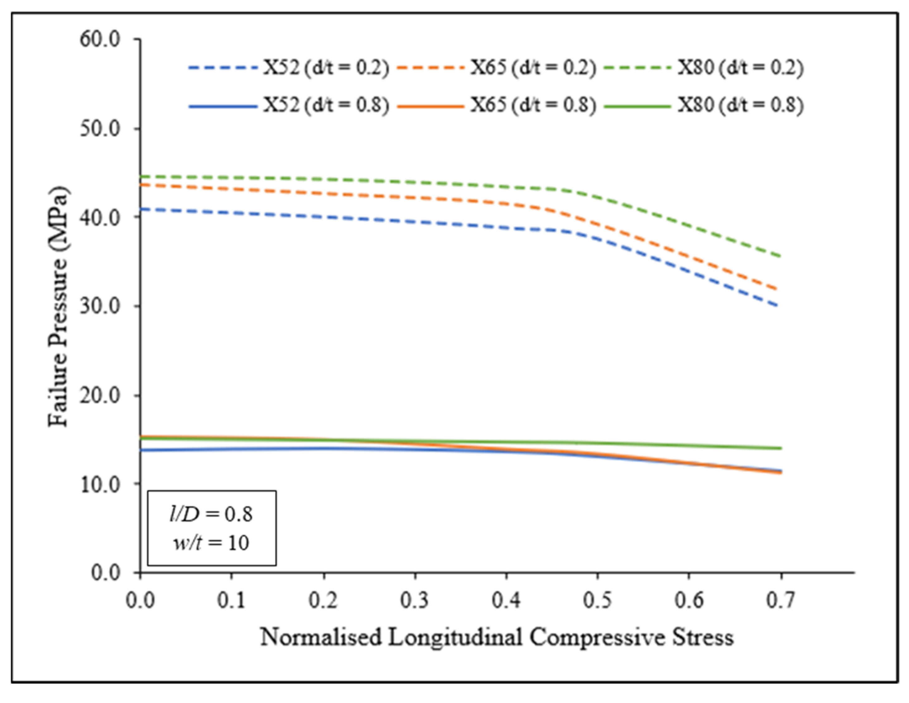
Figure 11 shows the effect of longitudinal compressive stress on failure pressure for a corroded pipeline with 0.2 and 0.8 $d/t$ normalised defect depths when the defect length was fixed at 0.8 $l/D$ and defect width was fixed at 10 $w/t$. The trendlines in Figure 11 demonstrate the same trend across all three types of material for both shallow and deep corrosion defects. The failure pressure of pipelines with deep corrosion defects was significantly lower (on average −65.90%) than the failure pressure of pipelines with shallow corrosion defects. This could be attributed to the higher stress concentration at the defect region for deeper corrosion defects. The failure pressure remained the same for longitudinal compressive stress of less than 0.4 ${\sigma }_c/{\sigma }_y$ for shallow corrosion defects, and then the failure pressure decreases linearly beyond 0.4 ${\sigma }_c/{\sigma }_y$. The failure pressure was not significantly reduced when the longitudinal compressive stress was increased in a pipeline with deep corrosion defects. Similar trends were observed for defect lengths of 0.2, 0.4, 1.0, and 1.2 $l/D$.

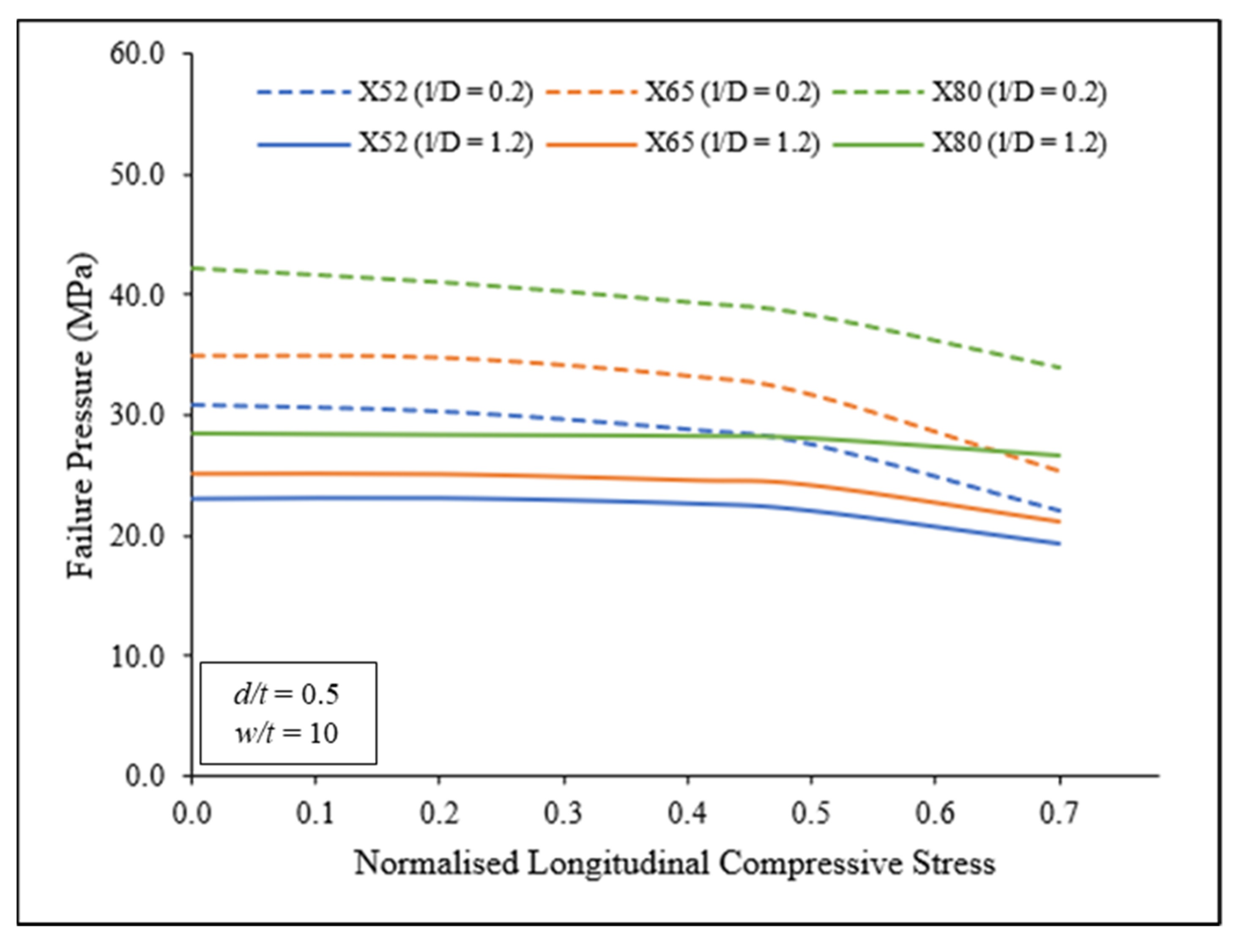
Figure 12 shows the effect of longitudinal compressive stress on failure pressure for a corroded pipeline with 0.2 and 1.2 $l/D$ normalised defect depths when the defect length was 0.5 $d/t$. The trendlines in Figure 12 demonstrate a similar pattern across all three types of material for both short and long corrosion defects. The failure pressure of long corrosion defects was lower (on average −25.00%) than the failure pressure of short corrosion defects, though it was not as significant as that shown in the trendlines of Figure 11. Similar trends were also observed for defect depths of 0.2, 0.4, 0.6, and 0.8 $d/t$.

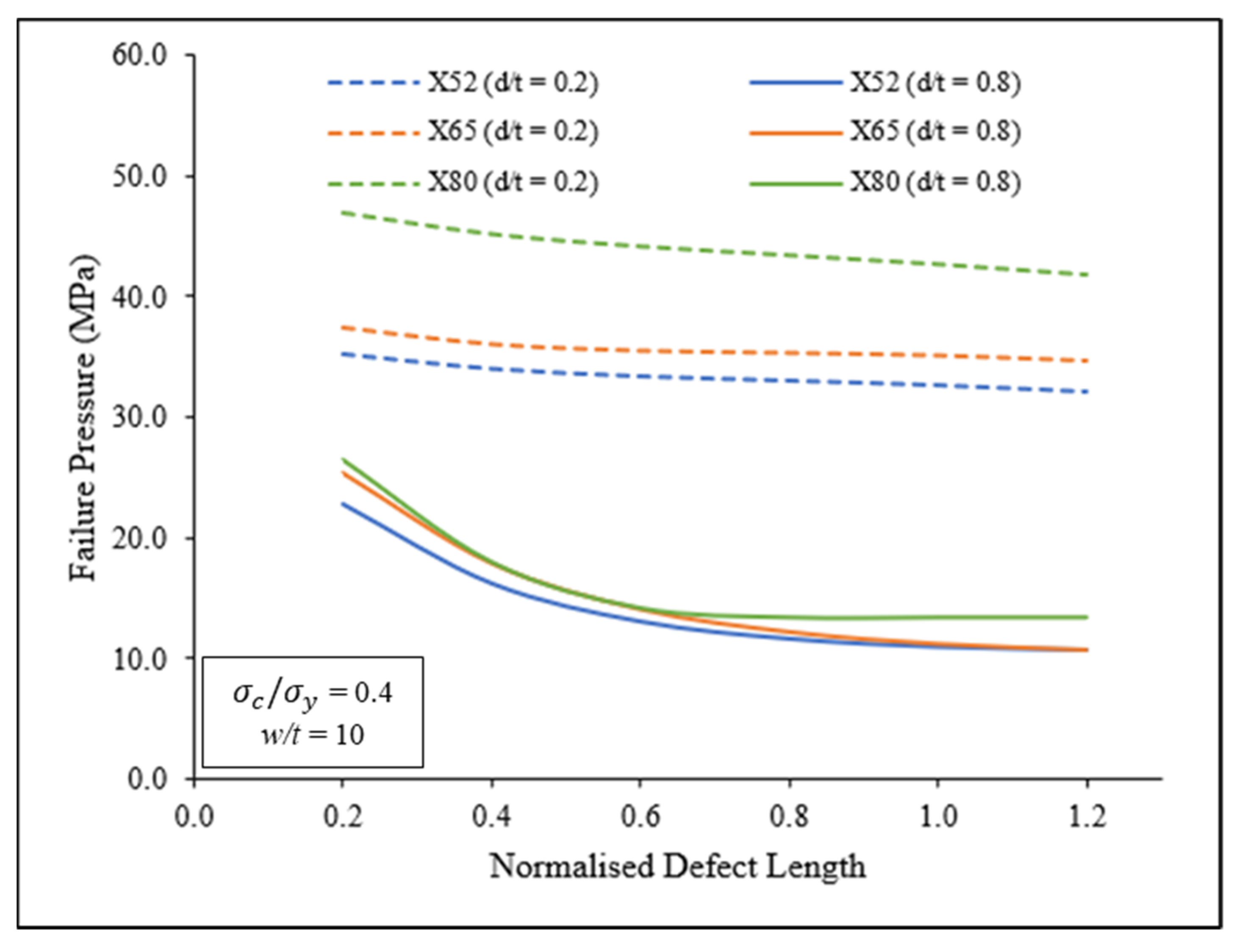
The effect of defect length on failure pressure for all three types of material is plotted in Figure 13, where the trendlines for 0.2 and 0.8 $d/t$ defect depths are compared at a fixed defect width of 10 $w/t$. Similar to the results shown in Figure 11, the failure pressure of a pipeline with deep defects was significantly lower (−66.91% on average) than failure the pressure of pipeline with shallow defects. Based on the trendlines of Figure 13, the failure pressure generally linearly decreased before plateauing at 0.8 $l/D$. For trendlines of 0.2 $d/t$, the average failure pressure reduction rates per 0.1 $l/D$ of the X52, X65, and X80 pipelines were −0.66%, −0.81%, and −1.03%, respectively. For trendlines with 0.8 $d/t$, the average failure pressure reduction rates per 0.1 $l/D$ of the X52, X65, and X80 pipelines were −2.17%, −1.84%, and −1.66%, respectively. The average failure pressure reduction rate increased from 0.2 to 0.8 $d/t$, which indicates that defect depth impacted failure pressure. The failure pressure of a pipeline with shallow corrosion defects slightly decreased when the defect length increased, but failure pressure of a pipeline with deep defects increased with the increasing defect length (up until the plateau point of 0.8 $l/D$). Similar trends were also observed for longitudinal compressive stresses of 0.0, 0.2, 0.5, and 0.7 ${\sigma }_c/{\sigma }_y$.

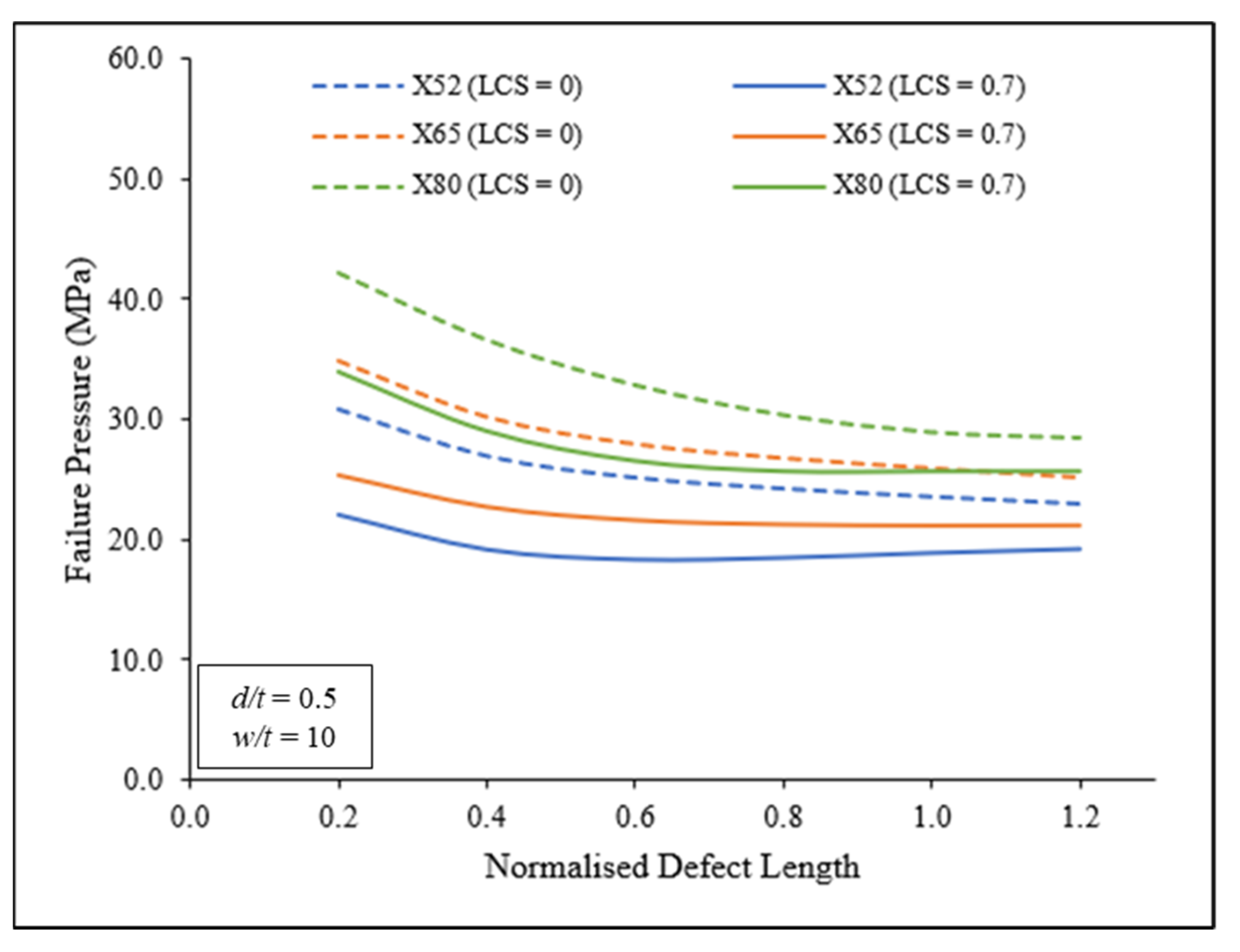
Figure 14 shows the effect of defect length on failure pressure for a corroded pipeline with 0.0 and 0.7 ${\sigma }_c/{\sigma }_y$ normalised longitudinal compressive stresses when the defect depth was fixed at 0.5 $d/t$. The trendlines in Figure 14 are similar to the trendlines in Figure 13, showing that failure pressure linearly decreased and then started to plateau at 0.8 $l/D$. The failure pressure difference between 0.0 and 0.7 ${\sigma }_c/{\sigma }_y$ was −20.79% on average. Longitudinal compressive stress did not influence the failure pressure as much as defect depth. Similar trends were also observed for defect depths of 0.2, 0.4, 0.6, and 0.8 $d/t$.

5. Conclusions

An artificial neural network-based equation for a corroded pipeline subjected to combined loadings was formulated in this study. An ANN model was trained with the FEA results of mid-to-high strength grade pipelines (API 5L X52, API 5L X65, and API 5L X80) with a single corrosion defect subjected to internal pressure and longitudinal compressive stress. The weights and biases of the network were used to formulate the assessment equation and evaluated with an unseen dataset. The percentage error of predictions based on the assessment equation ranged from −6.33% to 2.39%, with a standard deviation of 2.12, an R² value of 0.9975, an MSE of 0.000126, and an MAE of 0.00699. The assessment equation was subsequently used to perform a comprehensive parametric study to investigate the effect of material property, defect depth, defect length, and longitudinal compressive stress on the remaining strength of pipelines with single corrosion defects. In conclusion:

• The higher the strength of the pipeline, the higher its failure pressure when subjected to combined loadings. Here, X80 generally had the highest failure pressure, followed by X65 and X52.
• Defect depth had the most impact on reductions in failure pressure (average reductions of −65.90% and −66.91%), while longitudinal compressive stress (average reductions of −23.99% and −20.79%) and defect length (average reductions of −21.94% and −25.00%) had similar impacts on failure pressure.
• Across all three materials, the trend for failure pressure against defect depth, defect length, and longitudinal compressive stress exhibited similar patterns.

References

1. Han, C.J.; Zhang, H.; Zhang, J. Failure pressure analysis of the pipe with inner corrosion defects by FEM. Int. J. Electrochem. Sci. 2016, 11, 5046–5062. [Google Scholar] [CrossRef]
2. Cerit, M. Corrosion pit-induced stress concentration in spherical pressure vessel. Thin-Walled Struct. 2019, 136, 106–112. [Google Scholar] [CrossRef]
3. Bai, Y.; Bai, Q. 31—Subsea pipelines. In Subsea Engineering Handbook, 2nd ed.; Gulf Professional Publishing: Oxford, UK, 2019; pp. 919–940. [Google Scholar]
4. Grigory, S.C.; Smith, M.Q. Residual Strength of 48-Inch Diameter Corroded Pipe Determined by Full Scale Combined Loading Experiments. In Proceedings of the International Pipeline Conference, IPC, Calgary, AB, Canada, 9–13 June 1996; American Society of Mechanical Engineers Digital Collection: New York, NY, USA, 1996; pp. 377–386. [Google Scholar]
5. Xu, L.; Cheng, Y. Reliability and failure pressure prediction of various grades of pipeline steel in the presence of corrosion defects and pre-strain. Int. J. Press. Vessel. Pip. 2012, 89, 75–84. [Google Scholar] [CrossRef]
6. Seyfipour, I.; Bahaari, M.R. Analytical study of subsea pipeline behaviour subjected to axial load in free-span location. J. Mar. Eng. Technol. 2021, 20, 151–158. [Google Scholar] [CrossRef]
7. Bjørnøy, O.H.; Sigurdsson, G.; Cramer, E. Residual strength of corroded pipelines, DNV test results. In Proceedings of the Tenth International Offshore and Polar Engineering Conference, Seattle, WA, USA, 28 May–2 June 2000; International Society of Offshore and Polar Engineers: Mountain View, CA, USA, 2000. [Google Scholar]
8. Chauhan, V.; Swankie, T.; Espiner, R.; Wood, I. Developments in methods for assessing the remaining strength of corroded pipelines. In CORROSION 2009, Atlanta, Georgia, March 2009; NACE International: Houston, TX, USA, 2009. [Google Scholar]
9. Barbosa, A.; Teixeira, A.; Soares, C.G.; Li, M.; Kang, J.; Sun, L.; Wang, M.; Garbatov, Y. Strength analysis of corroded pipelines subjected to internal pressure and bending moment. In Proceedings of the Progress in the Analysis and Design of Marine Structures, Lisbon, Portugal, 8–10 May 2017; CRC Press: Boca Raton, FL, USA, 2017; pp. 803–812. [Google Scholar]
10. Belachew, C.T.; Ismail, M.C.; Karuppanan, S. Burst Strength Analysis of Corroded Pipelines by Finite Element Method. J. Appl. Sci. 2011, 11, 1845–1850. [Google Scholar] [CrossRef]
11. Smith, M.Q.; Grigory, S.C. New procedures for the residual strength assessment of corroded pipe subjected to combined loads. In Proceedings of the International Pipeline Conference, Calgary, AB, Canada, 9–14 June 1996; pp. 387–400. [Google Scholar]
12. Roy, S.; Grigory, S.; Smith, M.; Kanninen, M.F.; Anderson, M. Numerical Simulations of Full-Scale Corroded Pipe Tests with Combined Loading. J. Press. Vessel. Technol. 1997, 119, 457–466. [Google Scholar] [CrossRef]
13. Mohd, M.H.; Lee, B.J.; Cui, Y.; Paik, J.K. Residual strength of corroded subsea pipelines subject to combined internal pressure and bending moment. Ships Offshore Struct. 2015, 10, 554–564. [Google Scholar] [CrossRef]
14. Bruère, V.M.; Bouchonneau, N.; Motta, R.; Afonso, S.M.B.; Willmersdorf, R.B.; Lyra, P.R.M.; Torres, J.V.S.; De Andrade, E.Q.; Cunha, D.J.S. Failure pressure prediction of corroded pipes under combined internal pressure and axial compressive force. J. Braz. Soc. Mech. Sci. Eng. 2019, 41, 172. [Google Scholar] [CrossRef]
15. Han, L.; Han, L.; Liu, C. Neural network applied to prediction of the failure stress for a pressurized cylinder containing defects. Int. J. Press. Vessel. Pip. 1999, 76, 215–219. [Google Scholar] [CrossRef]
16. Khalajestani, M.K.; Bahaari, M.R.; Salehi, A.; Shahbazi, S. Predicting the limit pressure capacity of pipe elbows containing single defects. Appl. Ocean Res. 2015, 53, 15–22. [Google Scholar] [CrossRef]
17. Silva, R.; Guerreiro, J.; Loula, A. A Study of Pipe Interacting Corrosion Defects using the FEM and Neural Networks. Adv. Eng. Softw. 2007, 38, 868–875. [Google Scholar] [CrossRef]
18. Khalajestani, M.K.; Bahaari, M.R. Investigation of pressurized elbows containing interacting corrosion defects. Int. J. Press. Vessel. Pip. 2014, 123–124, 77–85. [Google Scholar] [CrossRef]
19. Arumugam, T.; Karuppanan, S.; Ovinis, M. Finite element analyses of corroded pipeline with single defect subjected to internal pressure and axial compressive stress. Mar. Struct. 2020, 72, 102746. [Google Scholar] [CrossRef]
20. Amaya-Gómez, R.; Sanchez-Silva, M.; Bastidas-Arteaga, E.; Schoefs, F.; Muñoz, F. Reliability assessments of corroded pipelines based on internal pressure—A review. Eng. Fail. Anal. 2019, 98, 190–214. [Google Scholar] [CrossRef]
21. British Standard Institution. Guide on Methods for Assessing the Acceptability of Flaws in Metallic Structures; British Standard Institution: London, UK, 1999. [Google Scholar]
22. Kim, Y.-J.; Oh, C.-S. Limit loads for pipe bends under combined pressure and in-plane bending based on finite element limit analysis. Int. J. Press. Vessel. Pip. 2006, 83, 148–153. [Google Scholar] [CrossRef]
23. Al-Owaisi, S.; Becker, A.; Sun, W. Analysis of shape and location effects of closely spaced metal loss defects in pressurised pipes. Eng. Fail. Anal. 2016, 68, 172–186. [Google Scholar] [CrossRef]
24. Baek, J.-H.; Kim, Y.-P.; Kim, W.-S.; Koo, J.-M.; Seok, C.-S. Load bearing capacity of API X65 pipe with dent defect under internal pressure and in-plane bending. Mater. Sci. Eng. A 2012, 540, 70–82. [Google Scholar] [CrossRef]
25. Choi, J.; Goo, B.; Kim, J.; Kim, Y.; Kim, W. Development of limit load solutions for corroded gas pipelines. Int. J. Press. Vessel. Pip. 2003, 80, 121–128. [Google Scholar] [CrossRef]
26. Xu, W.-Z.; Li, C.B.; Choung, J.; Lee, J.-M. Corroded pipeline failure analysis using artificial neural network scheme. Adv. Eng. Softw. 2017, 112, 255–266. [Google Scholar] [CrossRef]
27. Kim, Y.-P.; Kim, W.-S.; Lee, Y.-K.; Oh, K.-H. The Evaluation of Failure Pressure for Corrosion Defects within Girth or Seam Weld in Transmission Pipelines. In Proceedings of the 2004 International Pipeline Conference, Calgary, AB, Canada, 4–8 October 2004. [Google Scholar] [CrossRef]
Figure 1. Dimension of the model.
Applsci 12 01722 g001
Figure 2. Internal pressure and longitudinal compressive stress applied in the model.
Applsci 12 01722 g002
Figure 3. Pipe model meshed with elements.
Applsci 12 01722 g003
Figure 4. True stress–strain curve of API 5L X65 pipeline [25].
Applsci 12 01722 g004
Figure 5. ANN framework for this study.
Applsci 12 01722 g005
Figure 6. FFNN training process.
Applsci 12 01722 g006
Figure 7. The architecture of ANN in MATLAB.
Applsci 12 01722 g007
Figure 8. Regression plot of predicted normalised failure pressure by the assessment equations and FEA results for an unseen dataset.
Applsci 12 01722 g008
Figure 9. Failure pressure against normalised defect depth, with 0.0 and 0.7 normalised longitudinal compressive stresses for X52, X65, and X80.
Applsci 12 01722 g009
Figure 10. Failure pressure against normalised defect depth with 0.2 and 1.2 normalised defect lengths for X52, X65, and X80.
Applsci 12 01722 g010
Figure 11. Failure pressure against normalised longitudinal compressive stress with 0.2 and 0.8 normalised defect depths for X52, X65, and X80.
Applsci 12 01722 g011
Figure 12. Failure pressure against normalised longitudinal compressive stress with 0.2 and 1.2 normalised defect lengths for X52, X65, and X80.
Applsci 12 01722 g012
Figure 13. Failure pressure against normalised defect length with 0.2 and 0.8 normalised defect depths for X52, X65, and X80.
Applsci 12 01722 g013
Figure 14. Failure pressure against normalised defect length with 0.0 and 0.7 normalised longitudinal compressive stresses for X52, X65, and X80.
Applsci 12 01722 g014