Spatial Audio Scene Characterization (SASC): Automatic Localization of Front-, Back-, Up-, and Down-Positioned Music Ensembles in Binaural Recordings

Abstract

The automatic localization of audio sources distributed symmetrically with respect to coronal or transverse planes using binaural signals still poses a challenging task, due to the front–back and up–down confusion effects. This paper demonstrates that the convolutional neural network (CNN) can be used to automatically localize music ensembles panned to the front, back, up, or down positions. The network was developed using the repository of the binaural excerpts obtained by the convolution of multi-track music recordings with the selected sets of head-related transfer functions (HRTFs). They were generated in such a way that a music ensemble (of circular shape in terms of its boundaries) was positioned in one of the following four locations with respect to the listener: front, back, up, and down. According to the obtained results, CNN identified the location of the ensembles with the average accuracy levels of 90.7% and 71.4% when tested under the HRTF-dependent and HRTF-independent conditions, respectively. For HRTF-dependent tests, the accuracy decreased monotonically with the increase in the ensemble size. A modified image occlusion sensitivity technique revealed selected frequency bands as being particularly important in terms of the localization process. These frequency bands are largely in accordance with the psychoacoustical literature.

1. Introduction

While binaural audio technology has been known for decades [1], advancements in consumer electronics facilitated its widespread adoption predominantly during the post-millennial era. Nowadays, it is not only used in virtual reality applications and video games, but also supported by music and video streaming services [2]. Consequently, one can anticipate that large repositories of binaural audio recordings will be created soon, which will give rise to new challenges with the search and retrieval of “spatial audio information” from such recordings.

Building on Rumsey’s spatial audio scene-based paradigm [3], complex spatial audio scenes can be described at the three following hierarchical levels: (1) low level of individual audio sources, (2) mid-level of ensembles of sources, and (3) high level of acoustical environments. However, the state-of-the-art computational models for binaural localization developed so far were intended to localize individual audio sources [4,5,6,7,8,9] rather than to characterize complex spatial audio scenes at various descriptive levels (see [10] for the review of the binaural localization models). They were designed using predominantly speech signals and were intended to localize speakers [7]. Attempts to apply computational models for binaural localization to “music” audio signals are very rare [11,12]. Likewise, there are only a few developments [13] aiming to characterize complex spatial audio scenes at the mid- or high level, using the hierarchical paradigm described above [3]. Moreover, most of the binaural localization models developed so far are constrained to 2D localization in the horizontal plane [4,5,6,7,8,9]. Some preliminary models allowing for full-sphere binaural sound source localization have been proposed, only recently [14,15].

The goal of this study was to develop a method for the automatic localization of music ensembles using binaural signals, assuming that the ensembles are positioned in one of the following four locations with respect to the listener: front, back, up, and down (a music ensemble is understood as a group of musical sound sources, such as instruments or singers). It must be emphasized that the above task is not trivial, given the front–back and/or up–down confusion that might occur with human listeners in non-head-tracked binaural audio reproduction [16,17]. The idea of using the recordings exhibiting unusual placements of music ensembles may initially appear questionable, considering that in traditional music recordings, ensembles are typically positioned in front of a listener. However, since the state-of-the-art binaural systems enable sound engineers to “pan” foreground audio content behind, above, or below a listener, modern binaural recordings often involve unusual spatial scene arrangements.

In this work, the method employed to localize the ensembles was based on the convolutional neural network (CNN). In general, the proposed method could be employed in future systems intended for “spatial scene analysis” in binaural signals. In particular, it may facilitate the next generation of Internet search algorithms allowing their users to retrieve binaural music recordings exhibiting given spatial characteristics. It could also be used as a part of audio up-mixing algorithms (e.g., converting binaural signals to 22.2 audio format), providing such algorithms with information about the location of music ensembles. Furthermore, the proposed method could be employed as a part of an objective spatial audio quality assessment algorithm because of the reported interaction between spatial location of foreground audio objects and the perceived audio quality [18]. Additionally, it may help disambiguate front audio sources from back ones in algorithms localizing individual audio sources in binaural signals [19].

This study builds on our prior work. We already demonstrated that the traditional classification algorithm, employing a least absolute shrinkage and selection operator, could be used to identify three spatial audio scenes differing in horizontal distribution of foreground and background audio content around a listener in binaurally rendered recordings of music [20]. In the subsequent study [21], we compared the performance of humans against that of the machine learning algorithms in the task of the classification of spatial scenes in binaural recordings of music. The three scenes were subject to classification: (1) music ensemble located in the front, (2) music ensemble located at the back, and (3) music ensemble distributed around a listener. According to the results, the machine learning algorithms substantially outperformed human listeners. More recently, we compared the traditional classification methods with the deep learning one in the task of the classification of front- and back-positioned music ensembles [22]. The major drawback of the above-mentioned studies is that they were restricted to two-dimensional (2D) scenes, with the audio sources distributed solely within the horizontal plane (elevation angle was equal to 0°). The aforementioned limitation was overcome in the present work. To the best of the authors’ knowledge, this is the first study employing three-dimensional (3D) music ensembles (as opposed to 2D ones). Furthermore, it considers ensemble “size” as an experimental factor. Moreover, it attempts to identify the most important frequency bands, in terms of the spatial localization of the ensembles.

There is an increasing body of research focusing on “computational auditory scene analysis” (CASA) [23] and “acoustics scene classification” (ASC) [24]. The purpose of CASA is to isolate individual audio objects within a complex scene, whereas the aim of ASC is to identify acoustical environments. Therefore, despite their nomenclature similarity, the research goals within the above-mentioned areas are different from the one posed in this study, which is focused on the localization of music ensembles. The work reported in this paper constitutes part of the ongoing research project aiming to develop machine learning methods for the holistic characterization of spatial audio scenes of reproduced sound, referred to as spatial audio scene characterization (SASC) [25].

The paper is organized as follows. Section 2 gives an overview of the state-of-the-art models for binaural localization. A methodology outline is presented in Section 3. The audio repository employed in this work is described in Section 4. The topology of the CNN used in this study along with its development procedure is outlined in Section 5. The obtained results are presented in Section 6. Finally, the discussion of the achieved results and the conclusions are provided in Section 7 and Section 8, respectively.

2. State-of-the-Art Models for Binaural Localization

A machine learning approach is typically employed in modern computational models for binaural localization. The topology of these models typically includes an audio feature extractor followed by a classifier. Such features as the interaural level difference (ILD), interaural time difference (ITD), and interaural coherence (IC) [26] are typically calculated by the feature extractor. Then, the extracted features are fed to the input of classification algorithms, e.g., Gaussian mixture models [4]. More recently, deep learning techniques have been employed in the models [5,6,7,8]. It was recently demonstrated that the binaural localization models can benefit from using a source separation algorithm [12].

Binaural signals are normally subject to some forms of signal preprocessing prior to being used at the input of the deep neural networks. For example, instead of using the raw waveforms directly (such as in [9]), the standard features, such as ILD, ITD, and IC, could feed the network input [4]. Alternatively, the signals could be converted to spectrograms, which constitutes a common approach in the case of CNNs [27]. Due to the difficulty in the accurate estimation of ITD, particularly under noisy or reverberant conditions, raw values of the interaural cross-correlation function can be exploited at the input of the deep learning algorithms [6,8].

While the performance of the recently developed binaural models has been greatly improved, they still exhibit considerable errors attributed to a front–back confusion effect. To circumvent this issue, micro-head movements were modeled in some of the algorithms [4]. This solution is referred to as an “active” sound localization modeling [28]. Such an approach substantially reduces the front–back localization errors. However, it limits the applicability scope of the method, as it can only be employed in algorithms that allow for an adaptive synthesis of binaural signals [4], or it can be applied to systems equipped with robotic heads, such as those in [29]. For this reason, the method proposed in this paper was developed under the head-stationary condition (“passive” localization).

While the state-of-the-art models are capable of localizing speakers in concurrent speech binaural signals, they require a priori information on the “number” of audio sources present in a complex scene and their “characteristics” [4,5,6,7]. Such information is normally unavailable in the repositories of binaural music recordings on the Internet. Consequently, the method proposed in this paper is assumption free (“blind”) in terms of the number of music sources and their characteristics.

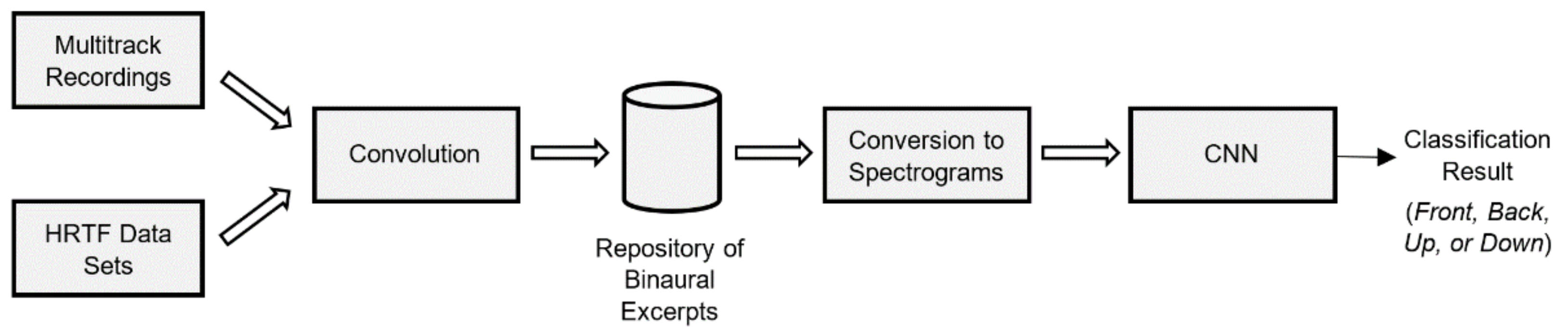
3. Methodology Overview

The methodology adopted in this study is outlined in Figure 1. In the first part of the study, the repository of the binaural excerpts was synthesized. To this end, the selection of the multitrack (monophonic) music recordings was convolved with the HRTF data sets. The binaural excerpts were synthesized in such a way that each recording exemplified one of the following four music ensemble locations: front, back, up, or down. Both the multitrack music recordings and the HRTF data sets were acquired from the publicly available repositories. In the second phase of the study, the binaural excerpts were converted to spectrograms and fed to the input of the convolutional neural network (CNN). The role of the CNN was to classify the recordings according to the location of the music ensembles (front, back, up, or down).

The procedure taken to synthesize the binaural excerpts is explained in detail in the subsequent section. The selection of the multitrack music recordings is described in Section 4.2, whereas the process of the selection of the HRTF data sets is included in Section 4.3. The convolution procedure is explained in Section 4.4. The procedure taken to divide the repository of the binaural excerpts into the train, validation, and test sets is provided in Section 4.5, followed by the description of the process of spectrograms generation (Section 4.6). The process of the CNN development and optimization is described in Section 5.

4. Synthesis of the Repository of Binaural Audio Recordings

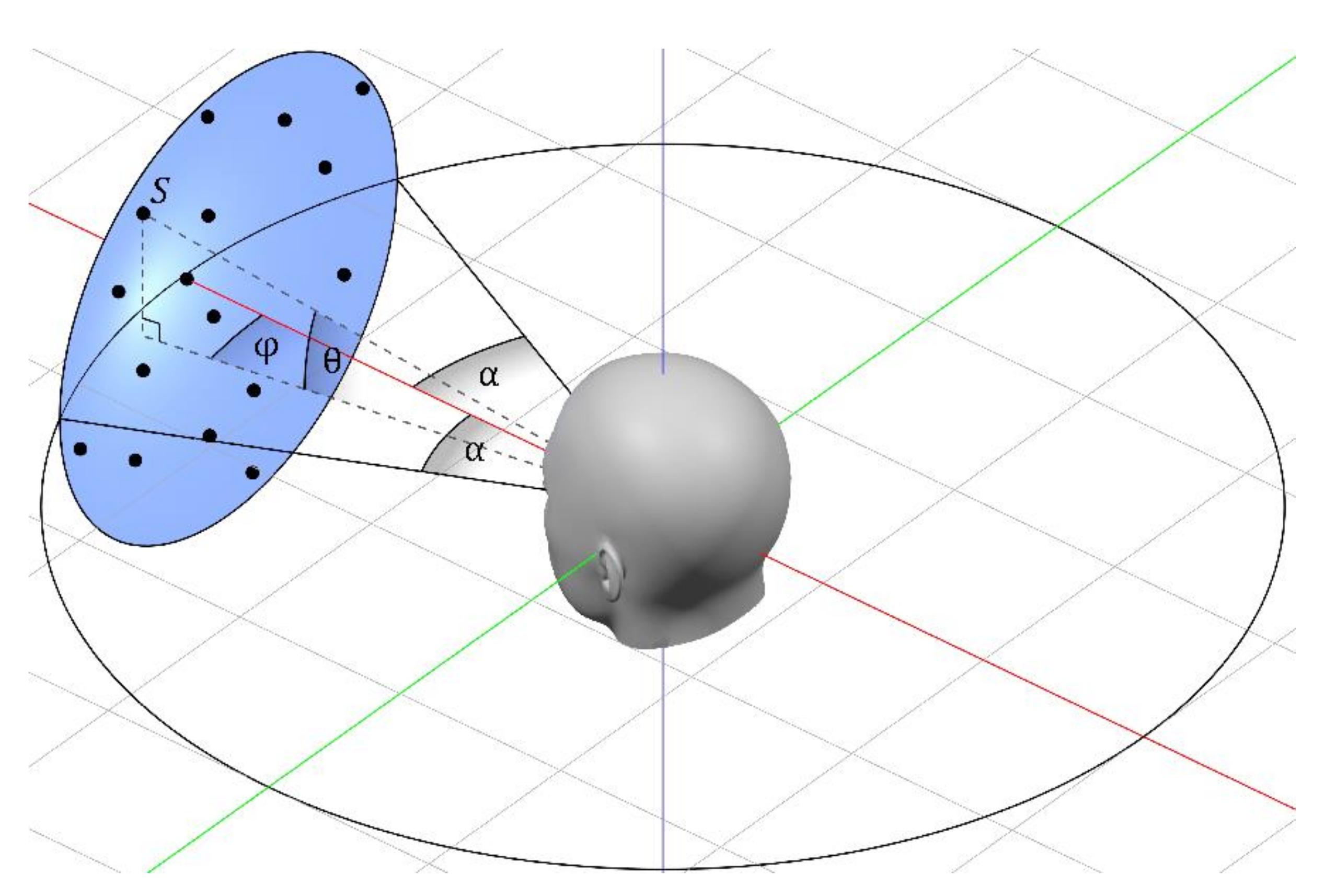
4.1. Composition of Spatial Audio Scenes

Prior to explaining the procedure taken for the synthesis of the binaural excerpts, the way that spatial scenes were composed must be described first. Figure 2 illustrates the convention used in this paper. Point S represents a selected individual audio source, be it a musical instrument or a vocalist, whose position is defined by the two coordinates: azimuth φ and elevation θ. As it can be seen, azimuth φ is measured counterclockwise with respect to a listener’s front-facing direction, whereas elevation is measured relative to a horizontal plane, with positive values for the upper hemisphere.

In this study, a music ensemble is defined as a group of sources, representing individual music instruments or singers, scattered on a spherical cap (a surface of a sphere cut by a plane). To a first approximation, it was assumed that a music ensemble had a circular boundary (in real-life recordings, the shape of ensembles could be elliptical or even irregular). An example of a front-located ensemble is depicted in Figure 2, with dots representing individual audio sources and a blue area illustrating an ensemble. The center of a cap is positioned at the intersection with the line indicating a front-facing direction. Note that the “size” of an ensemble is determined by angle α. Since the shape of an ensemble is circular, its width and height are equal. In this study, six values of an ensemble width were considered, namely ±15°, ±30°, ±45°, ±60°, ±75°, and ±90°. The last case represents an ensemble spanning a hemisphere.

In this work, four types of scenes were taken into consideration, with the ensembles located at the front, back, above, and below a listener, respectively. The procedure of “composing” the spatial scenes was as follows. First, a front-located ensemble was created by randomly generating the intended positions of individual audio sources within the ensemble boundary (with a uniform distribution). An ensemble located above a listener was generated by rotating the front-located ensemble by +90° in elevation. The ensemble located at the back of the listener was created as a mirror-like “image” of a front-located ensemble. In other words, there was a reflective symmetry between the front- and back-positioned ensembles. Likewise, an ensemble located below the listener was generated, using symmetric reflection of the above-located ensemble.

4.2. Multitrack Music Recordings

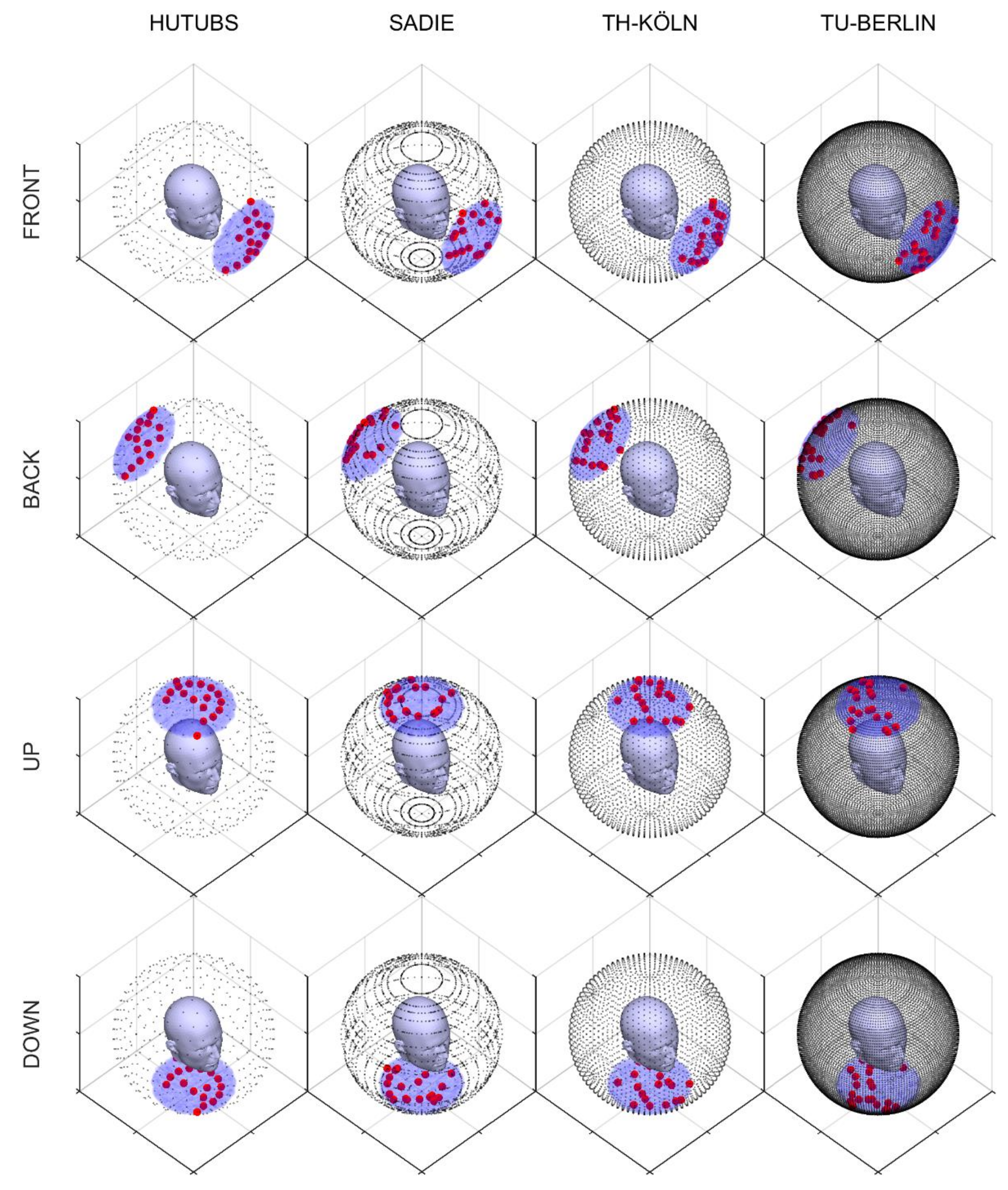
In total, 152 multitrack music recordings were used in the study. They represented a broad range of genres, including classical music, pop, orchestral, opera, rock, heavy metal, blues, jazz, country, dance, and electronica. The recordings were acquired from the publicly available repositories [30,31,32,33,34]. For most of the selected multitrack recordings, each track contained a monaural signal from a single musician or an individual musical instrument. If a given instrument was recorded on two or more tracks, the signals from these tracks were mixed with equal gains to a single monophonic track. Hence, it was assumed by the authors that every track used in this study represents an individual music audio source, be it a singer or a musical instrument. After such preprocessing, the number of the tracks within each recording ranged from 5 to 62, with a median value of 10.

4.3. HRTF Sets

The procedure for generating binaural excerpts (explained in detail in the next section) was based on the convolution of the individual music track signals with the head-related transfer functions (HRTFs). Twelve sets of HRTFs were selected for this study from the publicly available repositories (see

Table 1. HRTF sets used to synthesize binaural excerpts.

HRTF Set	Acronym	Head	Type	Radius	Source
1	HUTUBS	Subject pp2	Human	1.47 m	Huawei Technologies, TU Berlin, Munich Research Centre, Sennheiser Electronic [35]
2		Subject pp3
3		Subject pp4
4		Subject H3	Human
5	SADIE	Subject H4		1.2 m	University of York [36]
6		Subject H5
7		Neumann KU 100	Artificial	0.75 m	TH Köln, TU Berlin, TU Ilmenau [37]
8	TH KÖLN			1 m
9				1.5 m
10		FABIAN HATO 0°	Artificial	1.7 m	TU Berlin, Carl von Ossietzky University, RWTH Aachen University [38]
11	TU BERLIN	FABIAN HATO 10°
12		FABIAN HATO 350°

). The key requirement during the selection process was that the HRTFs must have contained the measurement points across a “full sphere,” in order to be able to synthesize 3D scenes with the ensembles located in the front, back, below, and above a listener. The first three HRTF sets adopted in this study were originally measured by Huawei Technologies, TU Berlin, Munich Research Centre, and Sennheiser Electronic (HUTUBS) [35]. The remaining nine HRTF sets were obtained at the University of York (SADIE) [36], TH Köln [37], and TU Berlin [38], respectively.

All the selected HRTF sets were measured in the anechoic chambers. The HUTUBS HRTFs were measured using the normalized least mean squares (NLMS) method [35], whereas the remaining HRTFs adopted in this study (SADIE, TH KÖLN, and TU BERLIN) were acquired by means of the sine sweep techniques [36,37,38]. Since the measurements could not be performed reliably at low frequencies, the impulse responses were compensated using various signal post-processing algorithms. For HUTUBS and SADIE HRTFs, the impulse responses were compensated below 200 Hz [35,36], whereas for TH KÖLN, they were compensated below 400 Hz [37].

Figure 3 illustrates the spatial resolution of the four example HRTF sets. Black dots surrounding a listener represent a grid of the measured HRTFs. The highest spatial resolution, being equal to 2° both in azimuth and elevation, was exhibited by HRTF sets taken at TU Berlin. The HRTF sets measured at University of York (SADIE) had the lowest elevational resolution. While their azimuthal resolution was still relatively high, ranging from 0.4° to 5°, their elevational resolution was low, as it varied from 2.5° up to 15°. Nevertheless, it was deemed adequate for our purposes.

In order to ensure the generalizability property of the developed model, the selected HRTFs were diverse in terms of the heads used to undertake the measurements. As it is presented in Table 1, the HRTF sets were obtained using human heads as well as artificial ones (KU 100 and FABIAN). The measurement radius varied between 0.75 and 1.7 m. HRTF sets 7–9 were obtained using only the head (without a torso), whereas the remaining nine HRTF sets were measured using both the head and the torso. The lack of a torso could have had a detrimental effect on the synthesis of ensembles located below and above the listener (this experimental factor is examined below in the results section).

For the last two HRTF sets presented in Table 1, the artificial head was originally rotated in azimuth relative to the torso by 10° and −10°, respectively. These rotations were compensated so that the heads in both cases were pointing forward. This was achieved by a counter-rotation of the two HRTF sets by −10° and 10° in azimuth, respectively. While such a procedure “equalized” the position of the head to a front-facing direction, it could have introduced some asymmetry to the ILD and ITD cues, due to the consequent torso rotations. However, since the magnitude of the torso rotations could be considered relatively small (±10°), these HRTF sets (after the head rotation compensation) were included in this study.

4.4. Convolution

As mentioned above, the binaural excerpts were synthesized by the convolution of the monophonic multitrack recordings with the HRTFs. This procedure was undertaken using the following equation:

$$y_c\left[n\right]={\displaystyle \sum }_{i=1}^N{\displaystyle \sum }_{k=0}^{K-1}{h}_{c,{\mathsf{\Theta }}_i,{\mathsf{\Phi }}_i}\left[n-k\right] x_i\left[k\right]$$

(1)

where $y_c\left[n\right]$ denotes an output binaural signal for an audio channel c (left or right) for a given music recording and sample n; $x_i\left[k\right]$ represents a k-th sample of an i-th monophonic track (individual music source); and $h_{c,{\mathsf{\Theta }}_i,{\mathsf{\Phi }}_i}\left[n\right]$ is a HRIR for an audio channel c, azimuth ${\mathsf{\Theta }}_i$ and elevation ${\mathsf{\Phi }}_i$ for an i-th monophonic track. As mentioned earlier, the total number N of the monophonic tracks varied across the music recordings, with a minimum value of 5 and a maximum of 62 (a median value was 10). The upper summation limit K was determined by the duration of the binaural excerpts (7 s) and amounted to 336 × 10³, given the sample rate of 48 kHz. It is assumed that the signals are in discrete-time domain.

Due to a relatively high spatial resolution of the HRTF sets selected for this study, no interpolation of HRTFs was performed. This means that for each individual track, an intended angle was “quantized” to that of the nearest HRTF within the measurement grid (constrained by the ensemble boundary). Figure 3 illustrates examples of individual music audio sources (red dots) within the front-, back-, up-, and down-located ensembles, respectively, after the quantization of the intended positions to the nearest available ones. Black dots represent the gird of the measured HRTFs. The figure shows the quantization effects for the four selected HRTF sets differing in their spatial resolution. In these examples, the width of the ensembles was fixed to ±30° as signified by blue areas.

All individual multitrack signals were RMS normalized prior to the convolution. The duration of each synthesized binaural excerpt was limited to 7 s. The excerpts were stored in two-channel uncompressed audio files with a 48 kHz sample rate and 32-bit resolution. In total, 43,776 binaural excerpts were synthesized (152 music recordings × 12 HRTF sets × 4 ensemble positions × 6 ensemble widths).

4.5. Data Splits

The whole repository of 43,776 excerpts was divided into development and test sets in the proportion of 74% to 26%. The former set was used for the development of the classification algorithm, whereas the latter one was solely exploited for its testing purposes (see Section 4.3 below). The development set was further subdivided into the train and validation sets. While the validation set was used to evaluate the performance of the network during its development, the purpose of the test set was to undertake its final assessment. The division of the data into the training, validation, and test sets constitutes one of the standard techniques used in machine learning, particularly in the case of large data sets. It is referred to as the three-way holdout method [39]. The number of excerpts and the number of music recordings allocated to the train, validation, and test sets are given in

Table 2. The division of the repository between the train, validation, and test sets.

	Development		Test
	Train	Validation
Number of Excerpts	25,632	6624	11,520
Data Proportion	59%	15%	26%
Number of Music Recordings	89	23	40

. Note that the music recordings assigned to these three sets were unique (no music recordings were shared across the sets).

4.6. Spectrograms Extraction

The binaural excerpts were converted to spectrograms and subsequently used at the input of CNN. Two spectrograms were calculated for each recording. They were derived for the left and right channel signals, respectively. The procedure applied to calculate the spectrograms was undertaken according to the results of our former studies [21]. Namely, linear-frequency spectrograms were calculated using 40 ms time frames with a 50% overlap. The signals in each time frame were multiplied by a Hamming window. The number of frequency bands in the spectrograms was set to 150. The frequency range of the spectrograms was limited to 100–16,000 Hz. The spectrogram values were clipped below 90 dB relative to their maxima (it was assumed that the components below 90 dB with respect to the spectrograms’ peak values contained noise or artifacts related to the music recording process or the HRTF measurement procedures). The spectrograms were standardized (mean equalized and normalized to unity variance) before they were applied to the network input. The VOICEBOX toolbox [40] was used in MATLAB to calculate the spectrograms.

5. Convolutional Neural Network

5.1. Network Topology

The well-proven AlexNet topology [41] was adopted for this work. The network consisted of the five convolutional layers followed by the three fully connected layers, as illustrated in Figure 4. The figure shows the number of the convolutional filters in each layer along with the size of their kernels. All the convolutional kernels were symmetric (3 × 3) with the exception of the one used in the first convolutional layer, where the asymmetric kernel was exploited (3 × 2). The dimensions of the tensors processed by the network are indicated by the numbers positioned at the interconnections between the adjacent layers. It can be seen that the spectrograms were progressively down-sampled, in terms of their resolution, as a result of the max-pooling procedure undertaken in the three convolutional units (1, 2, and 5). Recall that the original resolution of the spectrograms fed to the network input was equal to 150 × 349 pixels.

A rectified linear unit (ReLU) was used in all the layers, except the last one, where the softmax function was applied. To accelerate the learning process, cross-channel normalization was performed in all the convolutional layers. The number of neurons used in the fully connected layers was much smaller compared to that of the original AlexNet [41], being set to 256, 128, and 4, respectively. To reduce the risk of the model overfitting, two drop-out layers were employed with a 50% drop-out rate. The role of the last layer was to signify the predicted ensemble location. The size of the employed network, in terms of the total number of trainable parameters, was equal to approximately 4 million.

5.2. Network Optimization

For the optimization purposes, the network was trained using the training set, and its performance was evaluated using the validation set (see Table 2). A grid search technique was used to optimize the learning rate and the total number of epochs. Due to the variance in the observed results, the grid search technique was repeated seven times, and the mean classification accuracy values were used to assess the outcomes. The learning rate values considered during the grid search procedure were selected from the set $l_r\in \left({10}^{-4},5\times {10}^{-4},{10}^{-3},5\times {10}^{-3}\right)$, whereas the total number of epochs were chosen from the set $n_{epoch}\in \left(10,20,30,40\right)$. The learning rate $l_r$ was halved every 10 epochs. The network was trained using the Adam [42] optimization algorithm, with cross-entropy chosen as a loss function. A batch size was set to 256. According to the results of the grid search procedure, the model provided the best classification accuracy (81.79%) for the learning rate equal to 0.001 and the total number of epochs set to 30. Therefore, these values were adopted in the final model described in the remainder of this paper.

The network was implemented in MATLAB using Deep Learning Toolbox. The computations were accelerated using two GPU units (NVIDIA RTX 2080).

5.3. Network Testing

Once the best values for the learning rate and the total number of epochs were established, the model was trained again using the whole development set, and its performance was evaluated using the test set (see Table 2). The accuracy metric, defined as the ratio of the correctly classified experts to their total number, was used to assess the performance of the model. Moreover, the confusion matrices were inspected. Furthermore, the precision, recall, and F1-score were examined for some conditions (in our study, we used the standard definitions of these metrics [43]).

Two strategies for the network testing were considered: HRTF-dependent and HRTF-independent tests. Under the HRTF-dependent test, a single model was trained using the development set and subsequently tested with the test set. The development and test sets shared common spatial characteristics, as the same HRTFs were used to synthesize the excerpts in both sets. Consequently, this testing strategy may yield inflated results due to the risk of the model overfitting. Therefore, in order to better assess the generalization property of the method, the network was also tested under the HRTF-independent condition, with the details provided below in Section 6.2 and Section 6.3

There is some inevitable variance in the outcomes of the CNN training, which could be attributed to random initialization of weights and biases, the randomness of the drop-out procedure, and randomness inherent to the learning (optimization) technique. Therefore, CNN was repeatedly trained and tested, with the mean accuracy values and standard deviations reported in this paper. For the HRTF-dependent tests, the number of repetitions was 10. However, for the HRTF-independent test, the number of repetitions was lower, being equal to 8. The reduced number of repetitions in the latter case could be justified by the higher computational load. While in the HRTF-dependent test, only a single model had to be tested, the HRTF-independent tests required four different models to be assessed (see the Results section for details).

6. Results

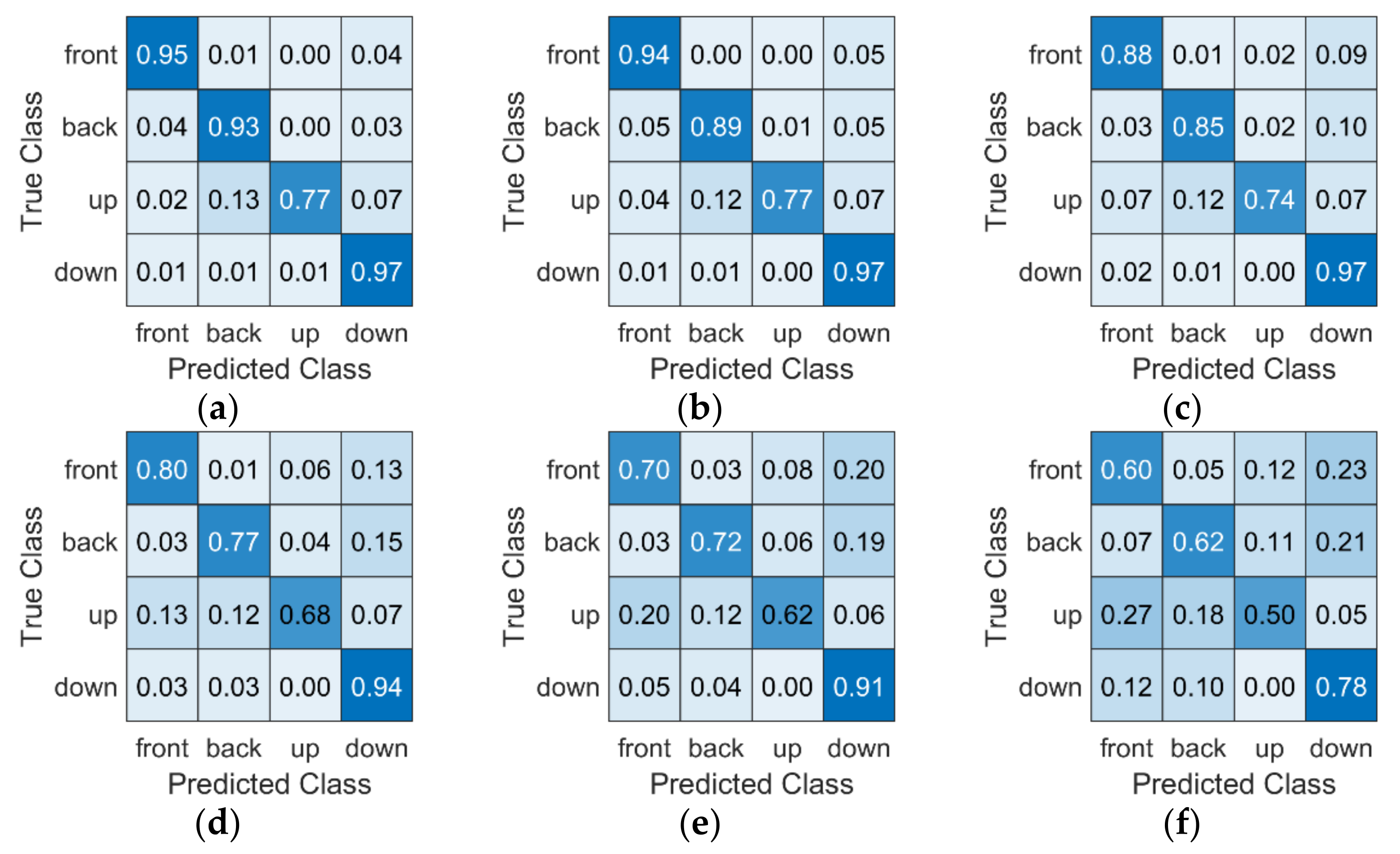
6.1. HRTF-Dependent Tests

According to the results obtained under the HRTF-dependent tests, the average accuracy of the classification of the front-, back-, up-, and down-located music ensembles was 80.26% (standard deviation (SD) 0.68). Further analysis revealed that the classification results depend on the two factors, namely (1) the width of the music ensembles and (2) the HRTF corpora used to synthesize the binaural excerpts, as illustrated in Figure 5. The four graphs presented in the figure correspond to the four HRTF corpora (HUTUBS, SADIE, TH-Köln, and TU-Berlin). Recall that each HRTF corpus contained a triplet of HRTF sets, as shown earlier in Table 1. It can be seen that the best accuracy scores were obtained for the narrowest ensembles (±15°). In this case, the mean classification accuracy scores were relatively high, ranging from 87.6% (for SADIE corpus) up to 91.9% (for TU-Berlin corpus), with an average score of 90.7% (SD 1.0).

According to the results depicted in Figure 5, the mean accuracy scores decrease monotonically with the increase in the ensemble width, reaching the lowest values for the ensembles occupying the whole hemispheres (±90°). While in this last-mentioned case, the observed accuracy scores are low, ranging from approximately 60% to 65%, they are still much higher than the no-information rate, which for this experiment was equal to 25% (a classification accuracy value obtained by chance). The deviation from the no-information rate was statistically significant at p < 0.001 according to the t-test. The likely reason for the observed effect of the monotonic decrease in the accuracy scores could be attributed to the less noticeable differences in spectral cues for the sources located near the edges of the “wide” ensembles (±60°, ±75°, and ±90°). For example, for the up and down ensembles, the differences between the spectrogram components for the sources located directly above and below a listener could be much more pronounced (e.g., due to a head and torso acoustical shadowing), compared to the sources located close to the equator.

Another interesting phenomenon that can be seen in Figure 5 is the disparity of the results for the two narrowest music ensembles (±15° and ±30°). For these two conditions, the mean accuracy scores obtained for SADIE corpus are approximately five points lower, compared that those obtained for the remaining three corpora (the differences are statistically significant at p < 0.001 according to the t-test). This effect is likely to be explained by the spatial sparsity of SADIE HRTFs near the zenith and nadir, as already illustrated in Figure 3 (recall that the HRTFs were not interpolated in this study). Out of four HRTF corpora used in this study, SADIE was the only one with sparse measurements in the vicinity of the zenith and nadir, potentially introducing some detrimental effects during the training of the model.

Figure 6 shows the example confusion matrices obtained for different ensemble widths under the HRTF-dependent test. It can be seen that regardless of the ensemble width, the down-located ensembles are identified the best (with the greatest number of correct classifications in the main diagonal cells). Moreover, it can be observed that CNN struggled to identify the ensembles located above the listener for all the considered ensemble widths.

Table 3. Classification results for the ensemble width of ±15°. Numbers in brackets represent standard deviations.

Ensemble Location	Precision [%]	Recall [%]	F1-Score [%]
front	93.5 (1.6)	95.4 (1.2)	94.4 (1.0)
back	85.6 (2.5)	93.1 (1.4)	89.2 (1.5)
up	98.9 (0.8)	77.5 (3.7)	86.8 (2.1)
down	87.5 (0.9)	96.9 (1.1)	92.0 (0.6)

shows the classification results for the ensemble width of ±15° (the best-case scenario) expressed in terms of the precision, recall, and F1-score. According to the table, the best overall results, using the F1-score as an indicator, were achieved for the front- and down-located ensembles. They were equal to 94.4% and 92%, respectively. While CNN exhibited exceptionally high precision for the ensembles located above the listener (98.9%), its recall was, in this case, relatively low (77.5%), giving a mediocre overall F1-score of 86.8%.

Table 4. Classification results for the music ensembles with the width of ±90°. Numbers in brackets represent standard deviations.

Ensemble Location	Precision [%]	Recall [%]	F1-Score [%]
front	57.3 (1.8)	60.1 (1.9)	58.6 (1.5)
back	64.5 (2.5)	61.6 (1.9)	63.0 (1.1)
up	69.1 (1.9)	50.2 (3.0)	58.1 (1.6)
down	61.3 (1.1)	77.6 (1.8)	68.5 (1.1)

shows the classification results for the ensemble width of ±90° (the worst-case scenario). It can be seen that the results are from 24 to 36 percentage points lower, compared to those obtained for the ensembles width of ±15°. Nevertheless, relatively satisfactory results were achieved for the down ensembles, with the F1-score of 68.5%.

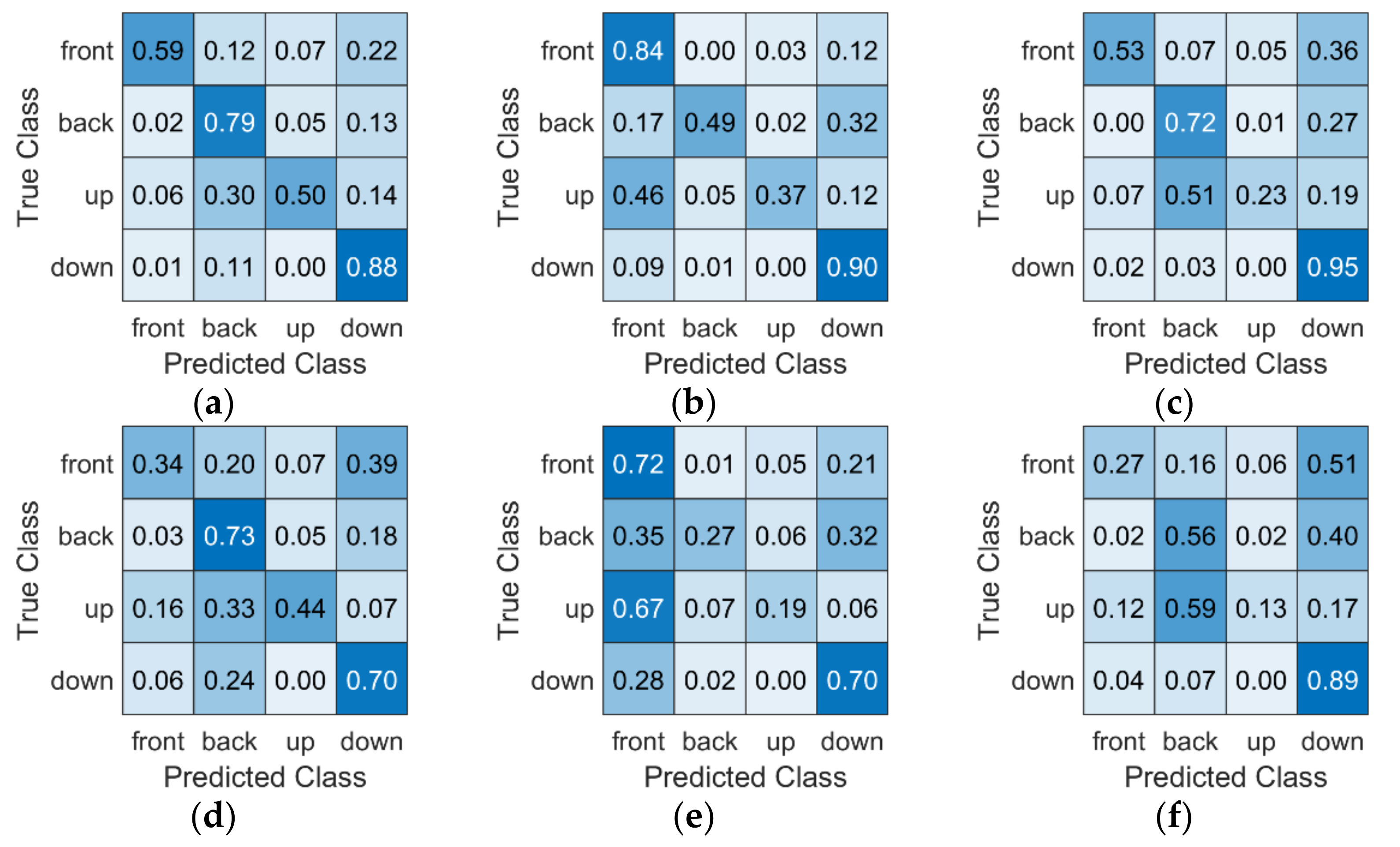
6.2. HRTF-Independent Tests

The previous section described the test results achieved when both the development and test sets contained the binaural excerpts synthesized using the same HRTFs. By contrast, this section presents the results for which the development and test sets comprised the excerpts synthesized with the “unique” HRTFs.

The procedure taken during the HRTF-independent tests was as follows. First, all the data were split into the development and test sets, using a similar method as that applied before for the HRTF-dependent test (see Table 2) but without dividing the development set into the training and validation sets. Recall that the music recordings allocated to the development and test sets were unique (in other words, the development and test sets were different in terms of the music content). Second, the data “within” the development and test sets were “filtered” using four different data folds, as shown in

Table 5. Data folds used for HRTF-independent tests.

Fold No.	HRTF Corpora Used for Development	HRTF Corpus Used for Testing
1	SADIE, TH-Köln, TU-Berlin	HUTUBS
2	HUTUBS, TH-Köln, TU-Berlin	SADIE
3	SADIE, HUTUBS, TU-Berlin	TH-Köln
4	SADIE, HUTUBS, TH-Köln	TU-Berlin

. For each fold, a single HRTF corpus was removed from the development set and used solely for testing purposes. For example, for fold No. 1, the excerpts synthesized using HUTUBS corpus were removed from the development set (leaving the excerpts convolved with the remaining three corpora), whereas the excerpts obtained with the HUTUBS corpus were solely retained in the test set. Consequently, for each fold, the development and test sets were mutually exclusive in terms of the HRTF corpora (in addition to being already music content-independent). A separate CNN model was developed and tested for each data fold. The above procedure was repeated eight times. The results presented below represent the mean values across the repetitions and associated standard deviations.

According to the results, for the narrowest ensembles (±15°), the average classification accuracy obtained under the HRTF-independent conditions was equal to 71.4% (SD 2.2). This result is 19.3 percentage points lower compared to that obtained earlier under the HRTF-dependent scenario. The observed difference was statistically significant at p < 0.001 according to t-test. This means that the outcomes of the HRTF-independent tests are more conservative compared to those achieved earlier under the HRTF-dependent tests. However, they better represent the generalization property of the developed method (capability to classify “unknown” samples).

Figure 7 shows the classification accuracy scores obtained under the HRTF-independent test conditions as a function of the ensemble width. In contrast to Figure 5, which presents the results for the single CNN model tested under the HRTF-dependent conditions, Figure 7 displays the results for four CNN models developed separately for each data fold listed in Table 5. The curves presented in the figure were annotated according to the corpus used for testing. For example, the results labeled as HUTUBS represent the accuracy scores obtained for the model which was developed using SADIE, TH-Köln, and TU-Berlin HRTF corpora and then tested on the excerpts synthesized using solely HUTUBS corpus (fold No. 1).

The main observation that can be made when inspecting the accuracy scores in Figure 7 is that they are approximately 10 to 20 percentage points lower compared to those presented earlier in Figure 5. Similar to the trend observed formerly under the HRTF-dependent test scenario, the accuracy scores also tend to decrease with the increase in the ensemble width. However, this effect is only noticeable for the relatively wide ensembles (±60°, ±75°, and ±90°). For the widest ensembles (±90°), the observed accuracy levels are relatively low, being equal to 55.5% for SADIE and approximately 47% for the remaining three HRTF corpora. Nevertheless, these classification levels considerably exceed the no-information rate (25%). The differences from the no-information rate are statistically significant at p < 0.001 according to the t-test. Note that for the ensemble widths of ±60° and ±75°, the results obtained for the TH-Köln corpus were lower compared to those obtained with the remaining three corpora (p < 0.001 according to the t-test). This indicates that the model trained with the binaural excerpts synthesized using HRTFs derived from “head and torso” do not always generalize well when applied for the excerpts convolved with the HRTFs measured solely with the head (without torso), which was the case for the TH-Köln corpus (in this instance, the Neumann KU 100 artificial head was used).

Figure 8 shows the selected examples of the confusion matrices obtained under the HRTF-independent tests. The top three matrices illustrate the results obtained for the ensemble width of ±60°, whereas the remaining three matrices characterize the results achieved for the ensemble width of ±90° (the worst-case scenario). While for the SADIE corpus (Figure 8a) the classification results could be considered relatively good, for the remaining conditions, CNN exhibited a substantial number of misclassifications, particularly for the widest ensemble width (±90°).

Table 6. Classification results for the ensemble width of ±60° for SADIE corpus. Numbers in brackets represent standard deviations.

Ensemble Location	Precision	Recall	F1-Score
front	86.6 (4.5)	59.4 (7.2)	70.3 (5.8)
back	60.3 (3.3)	79.3 (2.8)	68.4 (1.7)
up	80.0 (2.6)	50.0 (2.8)	61.5 (3.3)
down	64.1 (2.2)	87.7 (2.5)	74.0 (1.4)

shows the results obtained for SADIE corpus for the ensemble width of ±60° expressed in terms of the precision, recall, and F1-score. It can be seen that the classification results are relatively satisfactory, with an F1-score ranging from 61.5% (for up-located ensembles) to 74% (for down-located ensembles). By contrast, the results obtained for the TH-Köln corpus for the same ensemble width are worse (see

Table 7. Classification results for the ensemble width of ±60° for TH-Köln corpus. Numbers in brackets represent standard deviations.

Ensemble Location	Precision	Recall	F1-Score
front	85.8 (3.4)	52.6 (5.4)	65.0 (4.0)
back	54.2 (2.7)	72.1 (4.5)	61.8 (2.1)
up	81.7 (3.1)	22.9 (5.1)	35.5 (6.1)
down	54.1 (3.5)	95.3 (2.2)	68.8 (2.5)

), particularly for the up-located ensembles. For the aforementioned condition, recall was equal to only 22.9%, with an F1-score amounting to 35.5%.

6.3. Individual vs. Generalized HRTF Tests

This section presents the results of another form of the HRTF-independent tests. In contrast to the tests described in the previous section, a different strategy for creating data folds was pursued. The remaining aspects of the methodology were identical as before, and their description is omitted here. Instead of using four data folds as in the previous experiment, only two data folds were considered in the study. For the first data fold, the model was developed with the excerpts synthesized using the artificial (generalized) HRTFs, and then it was tested on the excerpts obtained with the human (individual) HRTFs. For the second data fold, the procedure was reversed. Namely, the model was developed exploiting the excerpts obtained with the human HRTFs and tested with the excerpts convolved with the artificial HRTFs (as before, for both folds, the development and test sets were unique in terms of the music content). Recall that HRTFs used in this study were selected in such a way that two corpora were obtained using human heads (HUTUBS and SADIE), whereas the remaining two ones were measured with the artificial heads (TH-Köln and TU-Berlin). Consequently, the proportion between the human and artificial HRTFs was balanced. For consistency with the previous section, the data folds used in this experiment are outlined in

Table 8. Data folds used for individual vs. generalized HRTF-independent tests.

Fold No.	HRTF Corpora Used for Development	HRTF Corpora Used for Testing
1	TH-Köln, TU-Berlin (Artificial Heads)	HUTUBS, SADIE (Human Heads)
2	HUTUBS, SADIE (Human Heads)	TH-Köln, TU-Berlin (Artificial Heads)

.

The obtained results are illustrated in Figure 9. The maximum average scores are similar to the ones described above, ranging between 70% and 80% (cf. Figure 7). Similar to the results seen in the previous section, the minimum scores are observed for the widest ensembles (±90°), being equal to approximately 50%. However, in contrast to the results discussed before, the maximum accuracy scores are not seen for the narrowest ensembles but for the ensembles having the widths of ±30° and ±45°, respectively, depending on the type of heads used for testing. Interestingly, while the two curves presented in Figure 9 show a relatively high correlation (overlap) for the ensemble widths between ±45° and ±90°, there are noticeable differences between the results for the two narrowest ensembles (±15° and ±30°). These differences are statistically significant at p < 0.001 according to the t-test. The above observation indicates that for the ensemble widths of ±15° and ±30°, the model developed with the excerpts synthesized using the human HRTFs generalizes better to the excerpts obtained with the artificial HRTFs than vice versa. This effect could be explained by the greater diversity of the human HRTFs used in this study compared to the artificial ones. Recall that the human HRTFs were derived from six human subjects, whereas the artificial HRTFs were measured using only two artificial heads (see Table 1). Greater diversity [44] within the HRTFs corpus can be conducive for the development of more generic binaural models [8].

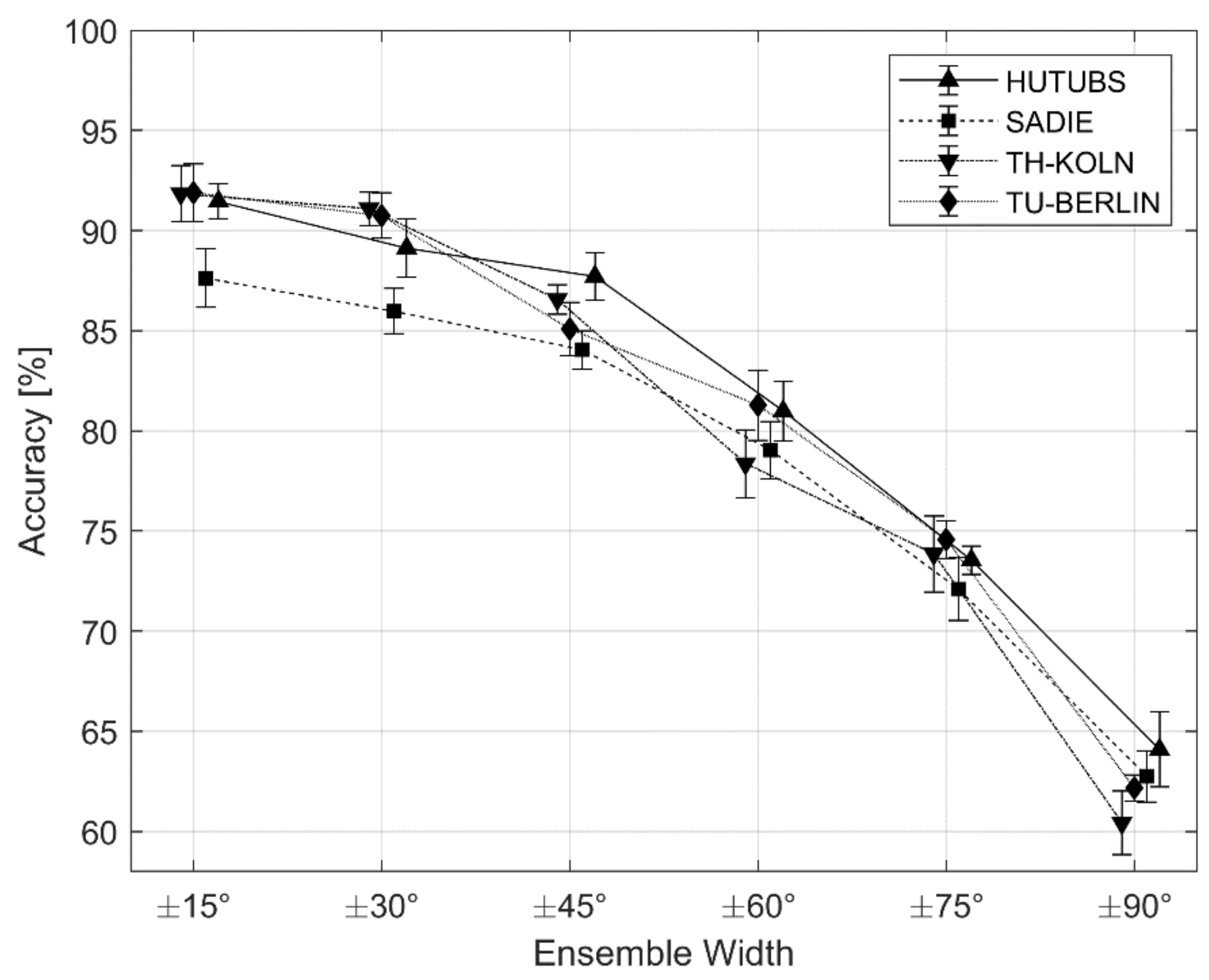
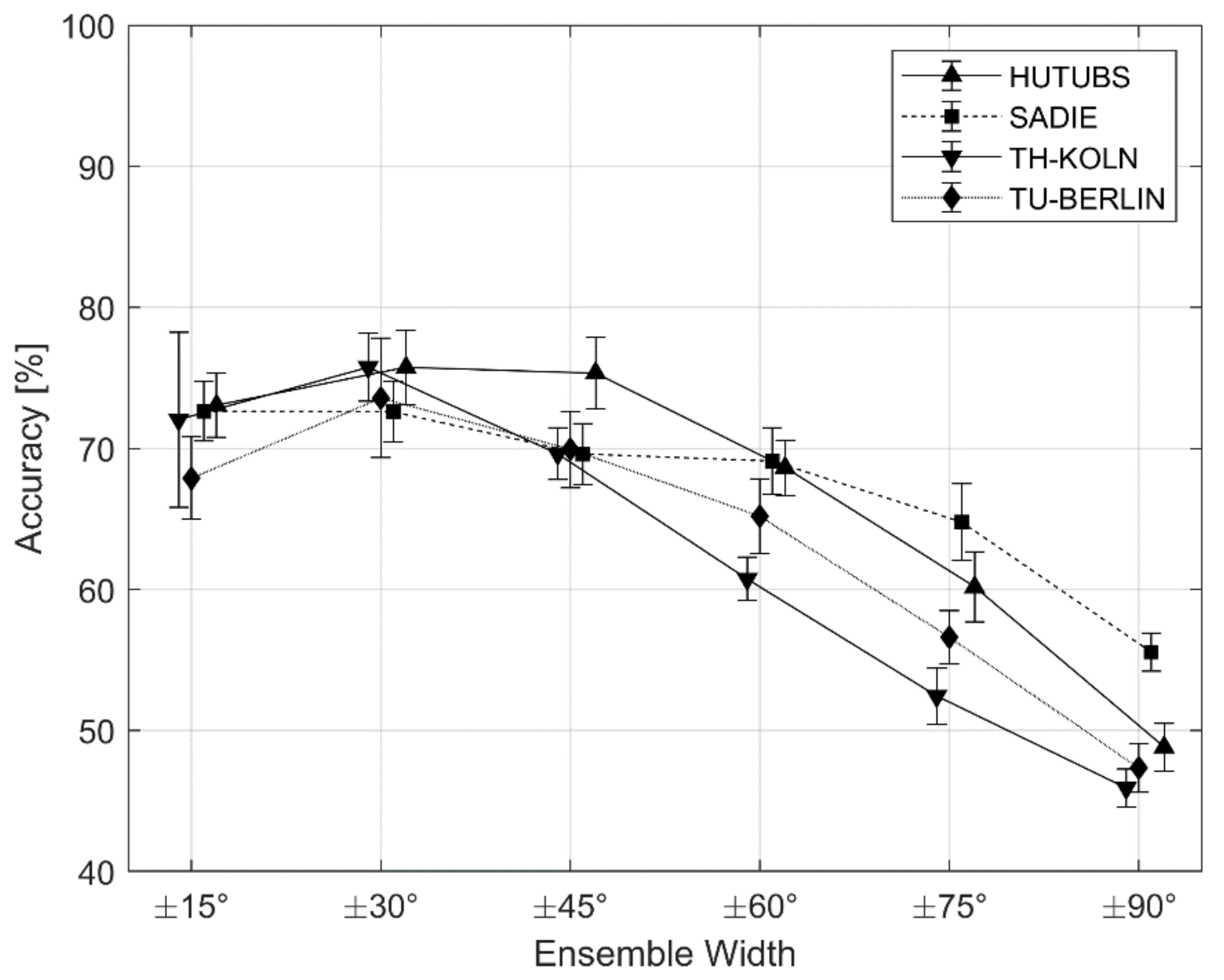
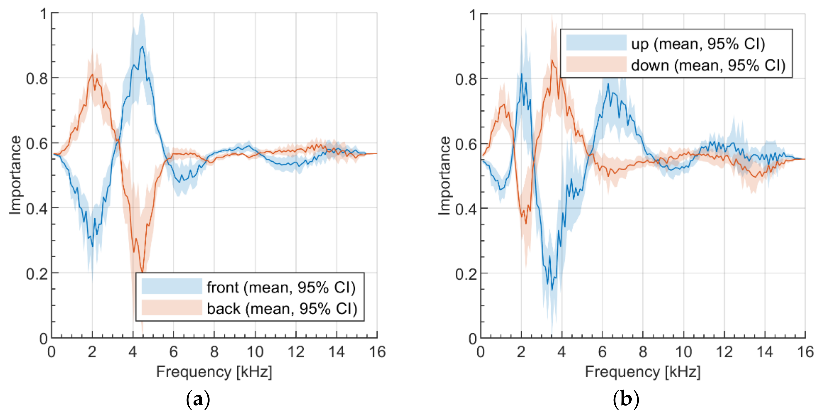
6.4. Follow-up Exploratory Study

In order to better understand how CNN performs the classification task, a popular gradient-weighted class activation mapping (Grad-CAM) technique [45] was trialed in the pilot tests (the results are not reported in the paper due to space limitations). This method highlights which parts of images constitute important regions in terms of the classification process. However, in our study, the Grad-CAM technique exhibited a relatively poor experimental repeatability, making it difficult to reach meaningful conclusions. Therefore, another visualization method was adopted for our purposes, namely, a modified version of the “occlusion sensitivity” technique [46]. In the occlusion sensitivity method, parts of the original input images are obscured, and the influence of such image degradation on the obtained results is quantified. This way, the sensitivity of the model to the occlusion of certain parts of the images can be ascertained. In the approach proposed in this study, instead of obscuring small parts of the images, it was decided to sequentially occlude selected frequency bands in the spectrograms (one frequency band at a time) and measure the sensitivity of the CNN model to such changes. The obtained results proved to be more repeatable compared to those obtained using the Grad-CAM technique. The modified occlusion sensitivity technique was applied to each excerpt within the binaural repository. Then, the results were averaged. In order to gauge how repeatable the method was, the above procedure was repeated 10 times, and the results were also averaged. The occlusion sensitivity technique was implemented in MATLAB.

The results obtained using the above modified occlusion sensitivity technique are presented in Figure 10. They are limited to the narrowest ensembles (width of ±15°). The graphs represent the average importance values and the associated 95% confidence intervals calculated across 10 experimental repetitions. The graphs were normalized to unity. An interesting phenomenon can be observed in these figures. Namely, for the ensembles located in the opposite directions (front–back or up–down), the importance curves are complementary to each other for most of the analyzed frequency spectrum (there is a certain degree of horizontal symmetry between the results). For example, for front ensembles, the maximum in the importance curve is seen at approximately 2 kHz, whereas its minimum falls at circa 4.5 kHz (see Figure 10a). A symmetrically “inverted” curve was obtained for the back ensembles, with its minimum and maximum being equal to approximately 2 kHz and 4.5 kHz, respectively. A similar complementary effect can also be observed for the up- and down-located ensembles (see Figure 10b). The symmetry effect can only be observed below approximately 7 kHz for front and back ensembles and below 5 kHz for up and down ensembles (it disappears above these frequencies).

According to the results obtained for the narrowest ensembles, presented in Figure 10a, the most important frequency region responsible for the localization of front ensembles ranges from approximately 3.5 kHz to 5 kHz, whereas the most important frequency region in terms of the localization of the back ensembles falls with the range between 1.5 kHz and 3 kHz. The results obtained for the up- and down-located ensembles of the same width (±15°) are different (Figure 10b). The most prominent frequency region related to the localization of the up ensembles fits within the range between 5.5 kHz and 8 kHz. The two important frequency bands can be identified in terms of the localization of the down ensembles. They fall within the frequency range of 0.5–1.5 kHz and 2.5–5 kHz, respectively.

Figure 11 shows similar graphs derived for the widest ensembles (width of ±90°). For the up and down ensembles (Figure 11a), the curves are similar as before (cf. Figure 10a). However, they exhibit more pronounced differences between the maxima and minima in the graphs. Likewise, the importance curve calculated for the down-located ensembles (Figure 11b) is similar to that derived for the narrowest ensemble. However, for the up-located ensembles, two prominent maxima emerged. They are located between the frequency bands of 1.5–2.5 kHz and 5.5–8 kHz, respectively.

7. Discussion

This work fits within an emerging field of spatial audio scene characterization (SASC). To the best of the authors’ knowledge, there are only three similar studies published so far. They are outlined in the first three rows in

Table 9. Overview of the studies regarding the automatic localization of music ensembles in binaural recordings.

Study	Impulse Response Type	Rendering Type	Ensemble Locations	Ensemble Width	Classification Method	Test Accuracy
						Room Dependent	Room Independent
Zieliński and Lee (2019) [20]	Reverberant (13 BRIRs)	2D	1. Front 2. Back 3. Front & Back	Fixed (±30°)	LASSO	76.9%	56.8%
Zieliński et al. (2020) [21]	Reverberant (13 BRIRs)	2D	1. Front 2. Back 3. Front & Back	Fixed (±30°)	Logit SVM XGBoost CNN	83.9% (SVM)	56.7% (Logit)
Zieliński et al. (2022) [22]	Anechoic (74 HRIRs)	2D	1. Front 2. Back	Fixed (±30°)	Logit SVM XGBoost CNN	99.4% (CNN)	94.5% (XGBoost)
This study	Anechoic (12 HRIRs)	3D	1. Front 2. Back 3. Up 4. Down	Varied (±15°, ±30°, ±45°, ±60°, ±75°, ±90°)	CNN	89.2% *	74.4% *

* For consistency with the previous studies, the accuracy values were calculated for ensemble width of ±30°.

. The accuracy levels obtained in this work for the room-dependent (HRTF-dependent) and room-independent (HRTF-independent) test conditions were equal to 89.2% and 74.4%, respectively, as shown in the last row of the table. For consistency of comparison, the above values were calculated for the ensemble width of ±30°. The outcomes obtained in this work may appear inferior relative to those attained in the third study and superior compared to those achieved in the first two studies shown in the table. However, due to the methodological differences, it is difficult to consistently compare the obtained results against those reported earlier in the literature. The main differences between the studies with the associated implications are discussed below.

The first two studies presented in Table 9 were based on the binaural excerpts synthesized using the reverberant room impulse responses (BRIRs), as opposed to the anechoic ones (HRIRs). Reverberant recordings are considered to be more challenging, in terms of the binaural audition modeling, than the anechoic ones [6]. Moreover, the studies differed with regards to the number of the impulse response sets exploited (be they HRIRs or BRIRs). Thirteen BRIR sets were incorporated in the first two studies presented in the table, whereas for the remaining two studies, the numbers of HRIR sets were equal to 74 and 12, respectively. Incorporating a greater number of HRIR sets tends to increase the localization accuracy both for the traditional and deep learning algorithms [22]. Therefore, it could be hypothesized that increasing the number of HRIRs (measured using different heads, microphones, and loudspeakers) could enhance the performance of the model developed in this work. The reason only 12 HRIRs were incorporated in the present study is due to the very limited number of publicly available three-dimensional HRIR sets.

The notable differences between the studies include the number of localization categories and the classification methods. The classification accuracy levels cannot be directly compared across the studies if a different number of classification categories (classes) is used. Note that that there were three localization categories (ensemble locations) incorporated in the first two studies, only two categories in the third study, and four categories in the present work (front, back, up, and down). It can be seen in Table 9 that the traditional classification methods were used in the first three studies. They comprised the least absolute shrinkage and selection operator (LASSO), logistic regression (Logit), support vector machines (SVM), and extreme gradient boosting (XGBoost). In addition, CNN was used in the second and the third studies. This work was solely based on CNN as the classification method due to its superior performance proven in the third study.

While the first three studies presented in Table 9 were concerned with the localization of the music ensembles solely in a horizontal plane (2D condition), this study is the first one incorporating the ensembles located on a sphere (3D condition). Moreover, for the first three studies, the width of the ensembles was restricted to ±30°, whereas in this study, the width (and height) of the ensembles varied between ±15° and ±90°. Consequently, it could be argued that incorporating three-dimensional ensembles varying in size introduced an additional difficulty in the development of the localization model in this study, potentially degrading its localization accuracy, compared to that reported in the previous three studies presented in Table 9.

The results of the modified image occlusion sensitivity technique showed that the frequency range between 3.5 kHz and 5 kHz is the most important in terms of the identification of the front ensembles. While caution should be exercised when comparing the “important” bands identified by the proposed algorithm with the results of the psychoacoustic studies in humans (machines could use their own specific way of decision making), the above frequency range is remarkably similar to one of the “boosted bands” associated with the localization of frontal sources as discovered by Blauert (3.6–5.8 kHz) [47]. According to this study, CNN used predominantly a frequency range between 1.5 kHz and 3 kHz to identify back ensembles. However, in this case, there is only a small overlap between the aforementioned band and another Blauert’s boosted band responsible for the localization of the back sources (0.72–1.7 kHz) [47]. As far as the localization of the up ensembles is concerned, in this work, a frequency range between 5.5 kHz and 8 kHz was identified as the most important. This outcome is similar to that obtained by Cheng and Wakefield [48], who concluded that frequencies near 6–8 kHz are thought to be important for elevation decoding. Moreover, they are consistent with the outcomes of the more recent study performed by Zonooz [49], who claimed that an elevation-dependent spectral notch is located between 6 kHz and 9 kHz (note that the peaks in the importance curves in Figure 10 may refer to information encoded both as spectral peaks or notches).

There are three limitations of the study that must be acknowledged. First, the impulse responses used to synthesize the binaural excerpts were anechoic. Therefore, it is unknown how the method would generalize to real-world binaural music recordings or to excerpts synthesized with “reverberant” binaural room impulse responses (BRIRs). Second, the boundary shape of the ensembles studied in this work was only circular. Extending the method by incorporating BRIRs and ensembles of arbitrary boundary shapes are left for future work. Third, the modified occlusion sensitive technique adopted in this study may potentially yield oversimplified results (since the method quantifies the influence of obscuring one frequency band at a time, it does not take into account any interactions between the frequency bands).

8. Conclusions

This work demonstrates that CNN is capable of undertaking the challenging task of identifying front, back, up, and down music ensembles in synthetically generated binaural signals, which constitutes the main contribution of this study to the field of spatial audio scene characterization (SASC). The classification accuracy scores obtained in this study could be considered satisfactory for narrow music ensembles (±15°), particularly when tested under the HRTF-dependent conditions. For these conditions, CNN yielded the classification accuracy equal to 90.7% (SD 1.0). The accuracy level decreased monotonically with the increase in the ensemble size, indicating that the method needs further improvements in terms of the classification of wider ensembles.

The results obtained under the HRTF-independent tests are approximately 10 to 20 percentage points lower compared to those achieved under the HRTF-dependent tests, implying that the generalization property of the developed method also needs to be enhanced. This could be accomplished by increasing the number of different HRTF sets employed in the development process. The results also suggest that the corpus of the HRTFs should be more diversified in terms of the types of the artificial heads used for their measurements.

In order to obtain a better insight as to how CNN undertook its classification process, a modified image occlusion sensitivity technique was applied. According to the results, several prominent frequency bands were identified in terms of the classification of the music ensembles (3.5–5 kHz for front ensembles, 1.5–3 kHz for back ensembles, 5.5–8 kHz for up ensembles, 0.5–1.5 kHz and 2.5–5 kHz for down ensembles). These frequency bands are largely in accordance with the psychoacoustical literature.

Future work regarding spatial audio scene characterization (SASC) may involve extending the model through incorporating reverberant BRIRs and by relaxing the current limitation of the method regarding the circular shape of the music ensemble boundaries.

References

1. Begault, D.R. 3-D Sound for Virtual Reality and Multimedia; NASA Center for AeroSpace Information: Hanover, MD, USA, 2000. [Google Scholar]
2. Kelion, L. YouTube Live-Streams in Virtual Reality and Adds 3D Sound, BBC News. Available online: http://www.bbc.com/news/technology-36073009 (accessed on 18 April 2016).
3. Rumsey, F. Spatial quality evaluation for reproduced sound: Terminology, meaning, and a scene-based paradigm. J. Audio Eng. Soc. 2002, 50, 651–666. [Google Scholar]
4. May, T.; Ma, N.; Brown, G.J. Robust localisation of multiple speakers exploiting head movements and multi-conditional training of binaural cues. In Proceedings of the IEEE International Conference on Acoustics, Speech and Signal Processing (ICASSP), South Brisbane, QLD, Australia, 19–24 April 2015; Institute of Electrical and Electronics Engineers (IEEE): Brisbane, Australia, 2015; pp. 2679–2683. [Google Scholar]
5. Ma, N.; Brown, G.J. Speech localisation in a multitalker mixture by humans and machines. In Proceedings of the INTERSPEECH 2016, San Francisco, CA, USA, 8–12 September 2016; pp. 3359–3363. [Google Scholar]
6. Ma, N.; May, T.; Brown, G.J. Exploiting Deep Neural Networks and Head Movements for Robust Binaural Localization of Multiple Sources in Reverberant Environments. IEEE/ACM Trans. Audio Speech Lang. Process. 2017, 25, 2444–2453. [Google Scholar] [CrossRef] [Green Version]
7. Ma, N.; Gonzalez, J.A.; Brown, G.J. Robust Binaural Localization of a Target Sound Source by Combining Spectral Source Models and Deep Neural Networks. IEEE/ACM Trans. Audio Speech Lang. Process. 2018, 26, 2122–2131. [Google Scholar] [CrossRef] [Green Version]
8. Wang, J.; Wang, J.; Qian, K.; Xie, X.; Kuang, J. Binaural sound localization based on deep neural network and affinity propagation clustering in mismatched HRTF condition. EURASIP J. Audio Speech Music Process. 2020, 2020, 4. [Google Scholar] [CrossRef] [Green Version]
9. Vecchiotti, P.; Ma, N.; Squartini, S.; Brown, G.J. End-to-end binaural sound localisation from the raw waveform. In Proceedings of the IEEE International Conference on Acoustics, Speech and Signal Processing (ICASSP), Brighton, UK, 12–17 May 2019; pp. 451–455. [Google Scholar]
10. May, T.; van de Par, S.; Kohlrausch, A. Binaural Localization and Detection of Speakers in Complex Acoustic Scenes. In The Technology of Binaural Listening, 1st ed.; Blauert, J., Ed.; Springer: London, UK, 2013; pp. 397–425. [Google Scholar]
11. Wu, X.; Wu, Z.; Ju, L.; Wang, S. Binaural Audio-Visual Localization. In Proceedings of the Thirty-Fifth AAAI Conference on Artificial Intelligence (AAAI-21), Virtual Conference, 2–9 February 2021. [Google Scholar]
12. Örnolfsson, I.; Dau, T.; Ma, N.; May, T. Exploiting Non-Negative Matrix Factorization for Binaural Sound Localization in the Presence of Directional Interference. In Proceedings of the IEEE International Conference on Acoustics, Speech and Signal Processing (ICASSP), Toronto, ON, Canada, 6–11 June 2021; Institute of Electrical and Electronics Engineers (IEEE): Toronto, Canada, 2021; pp. 221–225. [Google Scholar]
13. Nowak, J. Perception and prediction of apparent source width and listener envelopment in binaural spherical microphone array auralizations. J. Acoust. Soc. Am. 2017, 142, 1634. [Google Scholar] [CrossRef] [PubMed]
14. Hammond, B.R.; Jackson, P.J. Robust Full-sphere Binaural Sound Source Localization Using Interaural and Spectral Cues. In Proceedings of the IEEE International Conference on Acoustics, Speech and Signal Processing (ICASSP), Brighton, UK, 12–17 May 2019; pp. 421–425. [Google Scholar]
15. Yang, Y.; Xi, J.; Zhang, W.; Zhang, L. Full-Sphere Binaural Sound Source Localization Using Multi-task Neural Network. Proceedings of 2020 Asia-Pacific Signal and Information Processing Association Annual Summit and Conference (APSIPA ASC), Auckland, New Zealand, 7–10 December 2020; pp. 432–436. [Google Scholar]
16. Wenzel, E.M.; Arruda, M.; Kistler, D.J.; Wightman, F.L. Localization using nonindividualized head-related transfer functions. J. Acoust. Soc. Am. 1993, 94, 111–123. [Google Scholar] [CrossRef] [PubMed]
17. Jiang, J.; Xie, B.; Mai, H.; Liu, L.; Yi, K.; Zhang, C. The role of dynamic cue in auditory vertical localisation. Appl. Acoust. 2019, 146, 398–408. [Google Scholar] [CrossRef]
18. Zieliński, S.; Rumsey, F.; Kassier, R. Development and Initial Validation of a Multichannel Audio Quality Expert System. J. Audio Eng. Soc. 2005, 53, 4–21. [Google Scholar]
19. Usagawa, T.; Saho, A.; Imamura, K.; Chisaki, Y. A solution of front-back confusion within binaural processing by an estimation method of sound source direction on sagittal coordinate. In Proceedings of the IEEE Region 10 Conference TENCON, Bali, Indonesia, 21–24 November 2011; pp. 1–4. [Google Scholar]
20. Zieliński, S.K.; Lee, H. Automatic Spatial Audio Scene Classification in Binaural Recordings of Music. Appl. Sci. 2019, 9, 1724. [Google Scholar] [CrossRef] [Green Version]
21. Zieliński, S.K.; Lee, H.; Antoniuk, P.; Dadan, P. A Comparison of Human against Machine-Classification of Spatial Audio Scenes in Binaural Recordings of Music. Appl. Sci. 2020, 10, 5956. [Google Scholar] [CrossRef]
22. Zieliński, S.K.; Antoniuk, P.; Lee, H.; Johnson, D. Automatic discrimination between front and back ensemble locations in HRTF-convolved binaural recordings of music. EURASIP J. Audio Speech Music Process. 2022, 2022, 3. [Google Scholar] [CrossRef]
23. Szabó, B.T.; Denham, S.L.; Winkler, I. Computational models of auditory scene analysis: A review. Front. Neurosci. 2016, 10, 1–16. [Google Scholar] [CrossRef] [PubMed] [Green Version]
24. Barchiesi, D.; Giannoulis, D.; Stowell, D.; Plumbley, M.D. Acoustic scene classification: Classifying environments from the sounds they produce. IEEE Signal. Process. Mag. 2015, 32, 16–34. [Google Scholar] [CrossRef]
25. Zieliński, S.K. Spatial Audio Scene Characterization (SASC). Automatic Classification of Five-Channel Surround Sound Recordings According to the Foreground and Background Content. In Multimedia and Network Information Systems, Proceedings of the MISSI 2018, Wrocław, Poland, 12–14 September 2018; Advances in Intelligent Systems and Computing; Springer: Cham, Switzerland, 2019. [Google Scholar]
26. Blauert, J. Spatial Hearing. The Psychology of Human Sound Localization; The MIT Press: London, UK, 1974. [Google Scholar]
27. Han, Y.; Park, J.; Lee, K. Convolutional neural networks with binaural representations and background subtraction for acoustic scene classification. In Proceedings of the Conference on Detection and Classification of Acoustic Scenes and Events, Munich, Germany, 16 November 2017; pp. 1–5. [Google Scholar]
28. McLachlan, G.; Majdak, P.; Reijniers, J.; Peremans, H. Towards modelling active sound localisation based on Bayesian inference in a static environment. Acta Acust. 2021, 5, 45. [Google Scholar] [CrossRef]
29. Raake, A. A Computational Framework for Modelling Active Exploratory Listening that Assigns Meaning to Auditory Scenes—Reading the World with Two Ears. Available online: http://twoears.eu (accessed on 19 November 2021).
30. Pätynen, J.; Pulkki, V.; Lokki, T. Anechoic Recording System for Symphony Orchestra. Acta Acust. United Acust. 2008, 94, 856–865. [Google Scholar] [CrossRef]
31. D’Orazio, D.; De Cesaris, S.; Garai, M. Recordings of Italian opera orchestra and soloists in a silent room. Proc. Mtgs. Acoust. 2016, 28, 015014. [Google Scholar]
32. Mixing Secrets for The Small Studio. Available online: http://www.cambridge-mt.com/ms-mtk.htm (accessed on 19 November 2021).
33. Bittner, R.; Salamon, J.; Tierney, M.; Mauch, M.; Cannam, C.; Bello, J.P. MedleyDB: A Multitrack Dataset for Annotation-Intensive MIR Research. In Proceedings of the 15th International Society for Music Information Retrieval Conference, Taipei, Taiwan, 27 October 2014. [Google Scholar]
34. Studio Sessions. Telefunken Elektroakustik. Available online: https://telefunken-elektroakustik.com/multitracks (accessed on 19 November 2021).
35. Brinkmann, F.; Dinakaran, M.; Pelzer, R.; Grosche, P.; Voss, D.; Weinzierl, S. A Cross-Evaluated Database of Measured and Simulated HRTFs Including 3D Head Meshes, Anthropometric Features, and Headphone Impulse Responses. J. Audio Eng. Soc. 2019, 67, 705–718. [Google Scholar] [CrossRef]
36. Armstrong, C.; Thresh, L.; Murphy, D.; Kearney, G. A Perceptual Evaluation of Individual and Non-Individual HRTFs: A Case Study of the SADIE II Database. Appl. Sci. 2018, 8, 2029. [Google Scholar] [CrossRef] [Green Version]
37. Pörschmann, C.; Arend, J.M.; Neidhardt, A. A Spherical Near-Field HRTF Set for Auralization and Psychoacoustic Research. In Proceedings of the 142nd Audio Engineering Convention, Berlin, Germany, 20–23 May 2017. [Google Scholar]
38. Brinkmann, F.; Lindau, A.; Weinzierl, S.; van de Par, S.; Müller-Trapet, M.; Opdam, R.; Vorländer, M. A High Resolution and Full-Spherical Head-Related Transfer Function Database for Different Head-Above-Torso Orientations. J. Audio Eng. Soc. 2017, 65, 841–848. [Google Scholar] [CrossRef]
39. Raschka, S. Model Evaluation, Model Selection, and Algorithm Selection in Machine Learning. arXiv 2018, arXiv:abs/1811.12808. [Google Scholar]
40. Brookes, M. VOICEBOX: Speech Processing Toolbox for MATLAB. Available online: http://www.ee.ic.ac.uk/hp/staff/dmb/voicebox/voicebox.html (accessed on 25 November 2021).
41. Krizhevsky, A.; Sutskever, I.; Hinton, G.E. ImageNet classification with deep convolutional neural networks. Commun. ACM 2017, 60, 84–90. [Google Scholar] [CrossRef]
42. Kingma, D.P.; Ba, J. Adam: A Method for Stochastic Optimization. Available online: https://arxiv.org/abs/1412.6980 (accessed on 25 November 2021).
43. Sokolova, M.; Lapalme, G. A systematic analysis of performance measures for classification tasks. Inf. Process. Manag. 2009, 45, 427–437. [Google Scholar] [CrossRef]
44. So, R.H.Y.; Ngan, B.; Horner, A.; Braasch, J.; Blauert, J.; Leung, K.L. Toward orthogonal non-individualised head-related transfer functions for forward and backward directional sound: Cluster analysis and an experimental study. Ergonomics 2010, 53, 767–778. [Google Scholar] [CrossRef] [PubMed]
45. Selvaraju, R.R.; Cogswell, M.; Das, A.; Vedantam, R.; Parikh, D.; Batra, D. Grad-CAM: Visual Explanations from Deep Networks via Gradient-Based Localization. In Proceedings of the IEEE International Conference on Computer Vision (ICCV), Venice, Italy, 22–29 October 2017. [Google Scholar]
46. Zeiler, M.D.; Fergus, R. Visualizing and Understanding Convolutional Networks. In Proceedings of the Computer Vision—ECCV 2014, Zurich, Switzerland, 6–12 September 2014; Fleet, D., Pajdla, T., Schiele, B., Tuytelaars, T., Eds.; Springer International Publishing: Cham, Switzerland, 2014; pp. 818–833. [Google Scholar]
47. Blauert, J. Sound localization in the median plane. Acustica 1969, 22, 205–213. [Google Scholar]
48. Cheng, C.I.; Wakefield, G.H. Introduction to Head-Related Transfer Functions (HRTFs): Representations of HRTFs in Time, Frequency, and Space. J. Audio Eng. Soc. 2001, 49, 231–249. [Google Scholar]
49. Zonooz, B.; Arani, E.; Körding, K.P.; Aalbers, P.A.T.R.; Celikel, T.; van Opstal, A.J. Spectral Weighting Underlies Perceived Sound Elevation. Sci. Rep. 2019, 9, 1642. [Google Scholar] [CrossRef] [Green Version]
Figure 1. Methodology outline.
Applsci 12 01569 g001
Figure 2. Composition of a scene containing a front-positioned music ensemble. Points represent individual audio sources (musical instruments or singers). Blue area illustrates a music ensemble.
Applsci 12 01569 g002
Figure 3. Examples of spatial scenes generated using four selected HRTFs. Black dots represent a grid of the measured HRTFs. Red dots signify music sound sources. Front, back, up, and down-located music ensembles of fixed width (±30°) are illustrated using blue areas.
Applsci 12 01569 g003
Figure 4. CNN topology used for the identification of the ensemble locations.
Applsci 12 01569 g004
Figure 5. Mean classification accuracy scores obtained under HRTF-dependent tests. Error bars represent standard deviations.
Applsci 12 01569 g005
Figure 6. Confusion matrices obtained for different ensemble widths under the HRTF-dependent tests: (a) ±15°, (b) ±30°, (c) ±45°, (d) ±60°, (e) ±75°, (f) ±90°.
Applsci 12 01569 g006
Figure 7. Mean classification accuracy scores obtained under HRTF-independent tests. Error bars represent standard deviations.
Applsci 12 01569 g007
Figure 8. Example confusion matrices obtained under the HRTF-independent tests: (a) ±60° SADIE, (b) ±60° TU-Berlin, (c) ±60° TH-Köln, (d) ±90° SADIE, (e) ±90° TU-Berlin, (f) ±90° TH-Köln.
Applsci 12 01569 g008
Figure 9. Mean classification accuracy scores obtained for human vs. artificial HRTF-independent tests. Sold line illustrates the results for CNN developed using the artificial HRTFs and tested with the human HRTFs. Dashed line signifies the reversed scenario (CNN developed with the human HRTFs and tested with the artificial ones). Error bars represent standard deviations.
Applsci 12 01569 g009
Figure 10. Importance of the frequency bands in terms of the discrimination between the ensemble locations based on the CNN sensitivity to obscuring the spectrograms obtained for: (a) front and back ensembles, (b) up and down ensembles. The graphs were derived for the narrowest ensembles (±15°). The curves indicate the mean values and associated 95% confidence intervals.
Applsci 12 01569 g010
Figure 11. Importance of the frequency bands in terms of the discrimination between the ensemble locations based on the CNN sensitivity to obscuring the spectrograms obtained for: (a) front and back ensembles, (b) up and down ensembles. The graphs were derived for the widest ensembles (±90°). The curves indicate the mean values and associated 95% confidence intervals.
Applsci 12 01569 g011