Article

SMC-CPHD Filter with Adaptive Survival Probability for Multiple Frequency Tracking

1
School of Mechanical Convergence System Engineering, Kunsan National University, Gunsan 54150, Korea
2
Department of Mechanical System Engineering, Kumoh National Institute of Technology, Gumi 39177, Korea
3
Department of Aeronautics, Mechanical and Electronic Convergence Engineering, Kumoh National Institute of Technology, Gumi 39177, Korea
4
Department of Aerospace Engineering and Automation and System Research Institute, Seoul National University, Seoul 08826, Korea
*
Authors to whom correspondence should be addressed.
Appl. Sci. 2022, 12(3), 1369; https://doi.org/10.3390/app12031369
Submission received: 12 December 2021 / Revised: 22 January 2022 / Accepted: 26 January 2022 / Published: 27 January 2022

Abstract

:
We propose a sequential Monte Carlo-based cardinalized probability hypothesis density (SMC-CPHD) filter with adaptive survival probability for multiple frequency tracking to enhance the tracking performance. The survival probability of the particles in the filter is adjusted using the pre-designed exponential function related to the distribution of the estimated particle points. In order to ensure whether the proposed survival probability affects the stability of the filter, the error bounds in the prediction process are analyzed. Moreover, an inverse covariance intersection-based compensation method is added to enhance cardinality tracking performance by integrating two types of cardinality information from the CPHD filter and data clustering process. To evaluate the proposed method’s performance, MATLAB-based simulations are performed. As a result, the tracking performance of the multiple frequencies has been confirmed, and the accuracy of cardinality estimates are improved compared to the existing filters.

1. Introduction

Research on multiple target tracking filters has been actively conducted in various fields as well as in the target tracking field [1,2,3,4,5,6,7,8,9,10,11,12,13]. In particular, multiple target tracking filters based on a random finite set (RFS) can be used in many applications because the filters can track targets, even if the number of targets is unknown or if the number of targets changes over time [14,15,16,17,18,19,20,21]. Using these characteristics, we have recently conducted research to estimate and to finally mitigate multiple frequencies using the cardinalized probability hypothesis density (CPHD) filter among the RFS-based filters when a global navigation satellite system (GNSS) signal is received with multiple interference signals [22]. Studies have also been conducted to enhance the cardinality estimate performance of the CPHD filter, which results in increasing the performance of frequency estimates [22]. However, the performance is still not perfect, and additional methods are needed to enhance the estimate performance of the filter and the cardinality estimate performance in real situations, especially when clutter is present. As part of these studies, in this paper, the adaptive survival probability is applied to the sequential Monte Carlo-based CPHD (SMC-CPHD) filter.
In the initial version of the RFS filters, most of the filters assumed that the probability of survival is constant [7,8,10,23]. However, in a case with clutter in the measurements, fixing the probability of survival to a constant value (relatively large value) prevents the survival intensity from properly reflecting the situation and affects the estimate performance of the filter. Therefore, it is necessary to adaptively apply the probability of survival according to the measurements including clutter within the specified boundary. To address this problem, the previous paper also suggested adaptively setting the probability of survival to the GM-PHD filter [24]. Here, the authors of [24] defined a simple survival model to adaptively compute the survival probability of the state variable according to moving direction and position. In the paper [25], only the probability of detection was adaptively set. The proposed methods in previous papers were limited in the applicable systems or performed probability adjustment based on the observation area.
Based on the existing research results, we propose an adjustment technique of adaptive survival probability to set the appropriate value of survival probability for the multiple frequency tracking system, where the probability of survival is changed to be inversely proportional to the exponential function according to the Euclidean distance between the posterior state and the particles. In order to evaluate whether or not the modified survival probability affects the stability of the filter, the error bounds in the prediction process are analyzed to verify the stability of the filter. In addition to adaptive survival probability, an inverse covariance intersection (ICI)-based compensation technique is added to improve cardinality tracking performance. The ICI method [26,27] is one of the latest methods in the sensor fusion field. The ICI method provides more precise fusion results than those obtained by conventional covariance intersection (CI) methods [27]. The compensation method with ICI fused two types of cardinality information using the ICI method, which were the cardinality information estimated from the CPHD filter and the cardinality information additionally generated to compensate for the original cardinality estimate.
The paper is organized as follows. The processing steps of the SMC-CPHD filter are reviewed in Section 2. The probability of survival points in the SMC-CPHD filter is proposed in Section 3. In addition, the convergence of the mean square estimate is proved in case the proposed survival probability is applied in the existing SMC-CPHD filter. Subsequently, in Section 4, cardinality compensation with the ICI method is additionally applied in the proposed filter structure to enhance the estimate performance of the cardinality. In Section 5, various simulations are performed to evaluate the proposed method’s performance, and it is confirmed that the proposed method has better performance compared with conventional filtering methods. Section 6 summarizes the conclusions.

2. Processing Steps of the SMC-CPHD Filter

The CPHD filter is used for tracking multiple frequencies and is designed with an SMC structure [10,23]. This section presents a brief review of the SMC implementation in the CPHD filter with the target birth density driven by measurements [23].
Suppose at time k there are n k targets with states x k , 1 , , x k , n k in a state space, X n x , and m k measurements, z k , 1 , , z k , m k , in an observation space, Z n z . Then, a multiple target state and a multiple target observation are, respectively, defined as the finite sets: X k = { x k , 1 , , x k , n k } F ( X ) and Z k = { z k , 1 , , z k , m k } F ( Z ) . The state vector, x = ( y , β ) , consists of the usual kinematic components denoted by y and a label β , which distinguishes between a newborn target ( β = 1 ) and a persistent target ( β = 0 ) [23]. The PHD intensity function, D k | k ( x | Z 1 : k ) D k | k ( x ) , is referred to as δ x ( x ) f k | k ( x | Z 1 : k ) δ X . ρ k | k ( n | Z 1 : n ) ρ k | k ( n ) is the cardinality distribution at time k and ρ Γ , k | k 1 ( n ) ρ Γ ( n ) is the cardinality distribution of new targets at time k . The CPHD filter jointly propagates D k | k ( x ) and ρ k | k ( n ) . In this Algorithm 1, as the adaptive survival probability is not applied, the assumption is that the survival probability is constant, p S ( x ) = p S .
At time k = 0 , it is assumed that ρ 0 | 0 ( n ) = 1 if n = 0 , and ρ 0 | 0 ( n ) = 0 if n = 1 , 2 , , n max ( n max denotes the targets’ maximum anticipated number), and D 0 | 0 ( y , 0 ) = D 0 | 0 ( y , 1 ) = 0 . The intensity function, D k | k ( x ) , is approximated by using the random particles. At time k 1 :
D k 1 | k 1 ( y , 0 ) n = 1 N k 1 p w k 1 , p ( n ) δ y k 1 , p ( n ) ( y )
D k 1 | k 1 ( y , 1 ) n = 1 N k 1 b w k 1 , b ( n ) δ y k 1 , b ( n ) ( y )
where δ y 0 ( y ) represents the Dirac delta function [8] { ( w k 1 , p ( n ) , y k 1 , p ( n ) ) } n = 1 N k 1 p and { ( w k 1 , b ( n ) , y k 1 , b ( n ) ) } n = 1 N k 1 b denote the weighted particle sets for persistent targets and newborn targets. N k 1 p and N k 1 b define the number of persistent target particles and newborn target particles.
The predicted cardinality distribution, ρ k | k 1 ( n ) , can be expressed by a convolution [10]:
ρ k | k 1 ( n ) = j = 0 n ρ S , k | k 1 ( j ) ρ Γ ( n j )
ρ S , k | k 1 ( j ) = l = j l ! j ! ( l j ) ! p S j ( 1 p S ) l j ρ k 1 | k 1 ( l )
For the predicted intensity function, the summation of D k 1 | k 1 ( y , 0 ) and D k 1 | k 1 ( y , 1 ) is preferentially conducted and can be presented by the union of two particle sets as follows:
{ ( w k 1 ( n ) , y k 1 ( n ) ) } n = 1 N k 1 = { ( w k 1 , p ( n ) , y k 1 , p ( n ) ) } n = 1 N k 1 p { ( w k 1 , b ( n ) , y k 1 , b ( n ) ) } n = 1 N k 1 b
The predicted intensity function, D k | k 1 ( y , 0 ) , can be approximately calculated by the particle set:
D k | k 1 ( y , 0 ) n = 1 N k 1 w k | k 1 , p ( n ) δ y k | k 1 , p ( n ) ( y )
y k | k 1 , p ( n ) ~ q k ( | y k 1 ( n ) , Z k )
w k | k 1 , p ( n ) = p S ( y k 1 ( n ) ) π k | k 1 ( y k | k 1 , p ( n ) | y k 1 ( n ) ) w k 1 ( n ) q k ( y k | k 1 , p ( n ) | y k 1 ( n ) , Z k )
For simplicity, the importance density is adopted as q k ( | y k 1 ( n ) , Z k ) = π k | k 1 ( | y k 1 ( n ) ) [25]. For β = 1 , the predicted intensity function, D k | k 1 ( y , 1 ) , is approximated as:
D k | k 1 ( y , 1 ) n = 1 N k 1 b w k | k 1 , b ( n ) δ y k | k 1 , b ( n ) ( y )
y k | k 1 , b ( n ) ~ b k ( | z )
w k | k 1 , b ( n ) = v k | k 1 b N k b
where b k ( | z ) denotes the newborn target density and depends on g k ( z | y ) and prior knowledge. N k b = M b m k defines the total number of newborn target particles and M b refers to the number of particles per newborn target.
The updated cardinality distribution, ρ k | k ( n ) , is calculated by:
ρ k | k ( n ) = ϒ k 0 [ D k | k 1 ; Z k ] ( n ) ρ k | k 1 ( n ) ϒ k 0 [ D k | k 1 ; Z k ] , ρ k | k 1
ϒ k u [ D k | k 1 , Z ] ( n ) = j = 0 min ( | Z | , n ) ( | Z | j ) ! ρ κ , k ( | Z | j ) P j + u n × 1 p D ( ) , D k | k 1 ( , 0 ) u ( j + u ) 1 , D k | k 1 ( , 1 ) + D k | k 1 ( , 0 ) n × e j ( Ξ k ( D k | k 1 , Z ) )
Ξ k ( D k | k 1 , Z ) = { 1 , κ k κ k ( z ) D k | k 1 ( , 1 ) + p D ( ) D k | k 1 ( , 0 ) , g ( z | ) : z Z }
e j ( Z ) = W Z , | W | = j ( ζ W ζ )
where g , f = f ( x ) g ( x ) d x , κ k ( z ) defines the PHD of clutter, p D , k ( x ) p D ( x ) refers to the detection probability, and g k ( z | x ) represents the measurement likelihood at time k . e j ( Z ) denotes the elementary symmetric function of order j for a finite set, Z [8].
The updated intensity function, D k | k ( y , 0 ) and D k | k ( y , 1 ) , can be respectively calculated by:
D k | k ( y , 0 ) n = 1 N k 1 w k | k , p ( n ) δ y k | k 1 , p ( n ) ( y )
w k | k , p ( n ) = ( 1 p D ( y k | k 1 , p ( n ) ) ) w k | k 1 , p ( n ) + z Z k p D ( y k | k 1 , p ( n ) ) g k ( z | y k | k 1 , p ( n ) ) w k | k 1 , p ( n ) θ ( z )
D k | k ( y , 1 ) n = 1 N k b w k | k , b ( n ) δ y k | k 1 , b ( n ) ( y )
w k | k , b ( n ) = z Z k w k | k 1 , b ( n ) θ ( z )
θ ( z ) = κ k ( z ) + n = 1 N k b w k | k 1 , b ( n ) + n = 1 N k 1 p D ( y k | k 1 , p ( n ) ) g k ( z | y k | k 1 , p ( n ) ) w k | k 1 , p ( n )
For resampling steps, the estimated number of persistent targets, v ^ k p = n = 1 N k 1 w k | k , p ( n ) , and the expected number of newborn targets, v ^ k b = n = 1 N k b w k | k , b ( n ) , are respectively calculated. The number of particles, N k p , is selected by [ M p v ^ k p ] , where [ ] denotes the nearest integer and M p is the number of particles per persistent targets. Two intensity functions of (16) and (18) are respectively resampled N k p and N k b times to eliminate the particles with small weights and multiply the particles with large weights.
After resampling steps, the intensity function, D k | k ( y , 0 ) and D k | k ( y , 1 ) , can be respectively approximated by:
D k | k ( y , 0 ) n = 1 N k p w k , p ( n ) δ y k , p ( n ) ( y )
D k | k ( y , 1 ) n = 1 N k b w k , b ( n ) δ y k , b ( n ) ( y )
where w k , p ( n ) = v ^ k p / N k p and w k , b ( n ) = v ^ k b / N k b .
The whole process of the SMC-CPHD filter is presented in detail in [23], and the SMC-CPHD filter’s pseudocode at time k is as shown below [23]:
Algorithm 1: SMC-CPHD filter
Inputs: cardinality distribution: ρ k 1 | k 1 ( n ) ,
              intensity function (case β = 0 ) :   D k 1 | k 1 ( y , 0 ) :   { ( w k 1 , p ( n ) , y k 1 , p ( n ) ) } n = 1 N k 1 p , Equation (1)
              intensity function (case β = 1 ) :   D k 1 | k 1 ( y , 1 ) :   { ( w k 1 , b ( n ) , y k 1 , b ( n ) ) } n = 1 N k 1 b , Equation (2)
              measurement set: Z k = { z k , 1 , , z k , m k }   ( m k = | Z k | )
predicted cardinality distribution: ρ k | k 1 ( n ) , Equation (3)
input particle sets: { ( w k 1 ( n ) , y k 1 ( n ) ) } n = 1 N k 1 , Equation (5)
predicted intensity function (case β = 0 ) :   D k | k 1 ( y , 0 ) , Equation (6)

for n = 1 , , N k 1 do
     y k | k 1 , p ( n ) ~ π k | k 1 ( | y k 1 ( n ) ) , Equation (7)
     w k | k 1 , p ( n ) = p S ( y k 1 ( n ) ) w k 1 ( n ) , Equation (8)
end for

number of newborn target particles: N k b = M b m k
predicted intensity function (case β = 1 ) :   D k | k 1 ( y , 1 ) , Equation (9)

for j = 1 , , m k do
  for l = 1 , , M b do
         n = l + ( j 1 ) M b
         y k | k 1 , b ( n ) ~ b k ( | z k , j ) , Equation (10)
         w k | k 1 , b ( n ) = v k | k 1 b / N k b , Equation (11)
    end for
end for

updated cardinality distribution: ρ k | k ( n ) , Equation (12)

for all   z Z k do
     Ξ k ( D k | k 1 , Z k \ { z } ) , Equation (14)
     e j ( Ξ k ( D k | k 1 , Z k \ { z } ) ) , Equations (14) and (15)
     ϒ k u [ D k | k 1 , Z k \ { z } ] ( n ) ,   Equation   ( 13 )   ( for   u = 1 , 0 )
end for

updated intensity function: D k | k ( y , 0 ) ,   D k | k ( y , 1 ) , Equations (16) and (18)
updated weights (case β = 0 ) :   w k | k , p ( n ) ,   n = 1 , , N k 1 , Equation (17)
updated weights (case β = 1 )   :   w k | k , b ( n ) ,   n = 1 , , N k b , Equation (19)
estimated number of persistent and newborn targets: v ^ k p = n = 1 N k 1 w k | k , p ( n ) ,   v ^ k b = n = 1 N k b w k | k , b ( n )
number of particles for resampling: N k p = [ M p v ^ k p ]
resample   N k p   times   from   { ( w k | k , p ( n ) / v ^ k p , y k | k 1 , p ( n ) ) } n = 1 N k 1   to   obtain   { ( w k , p ( n ) , y k , p ( n ) ) } n = 1 N k p
resample   N k b   times   from   { ( w k | k , b ( n ) / v ^ k b , y k | k 1 , b ( n ) ) } n = 1 N k b   to   obtain   { ( w k , b ( n ) , y k , b ( n ) ) } n = 1 N k b
Outputs: updated cardinality distribution: ρ k | k ( n ) ,  
updated intensity function: D k | k ( y , 0 ) :   { ( w k , p ( n ) , y k , p ( n ) ) } n = 1 N k p , Equation (21)

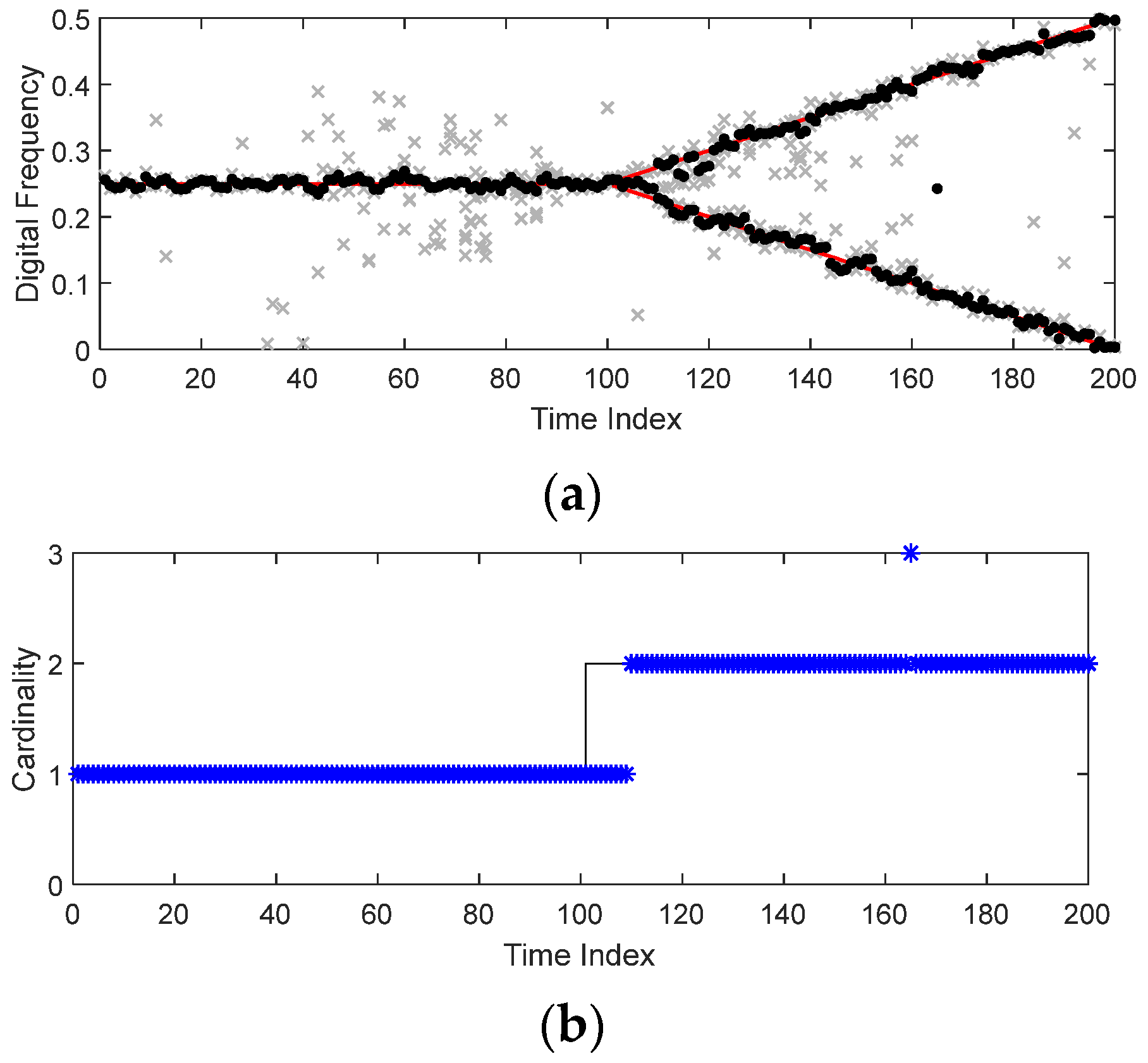
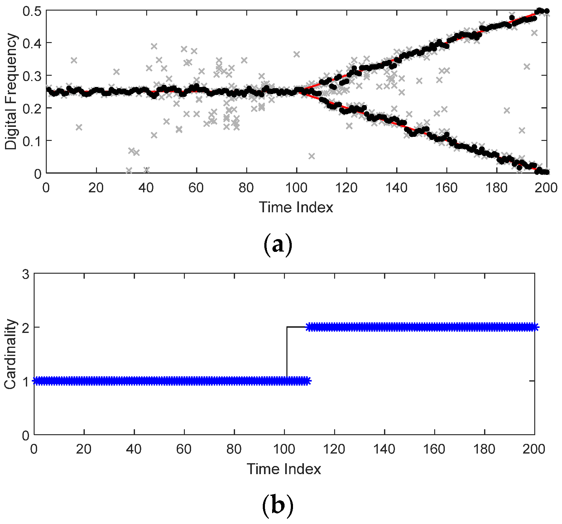
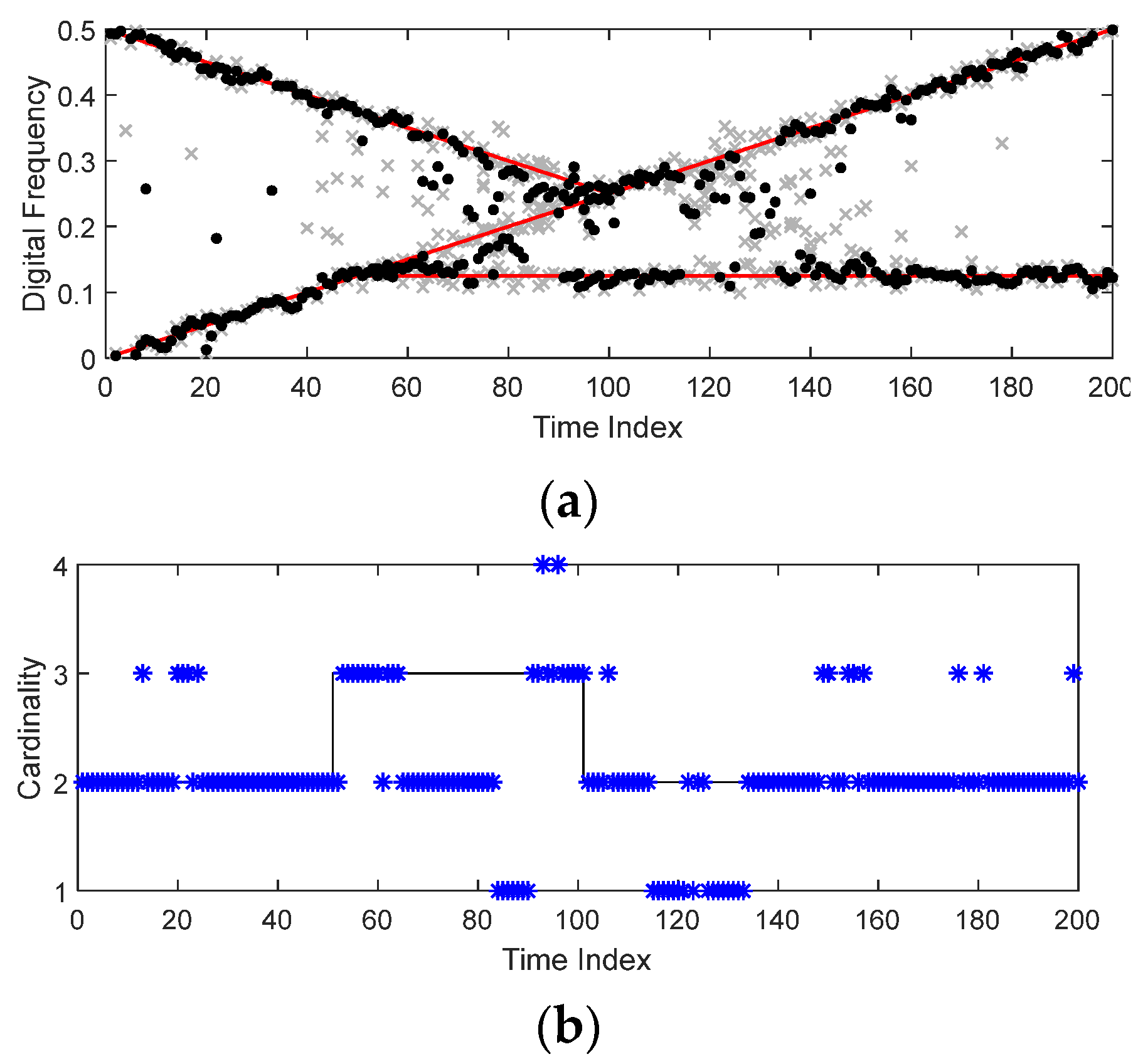
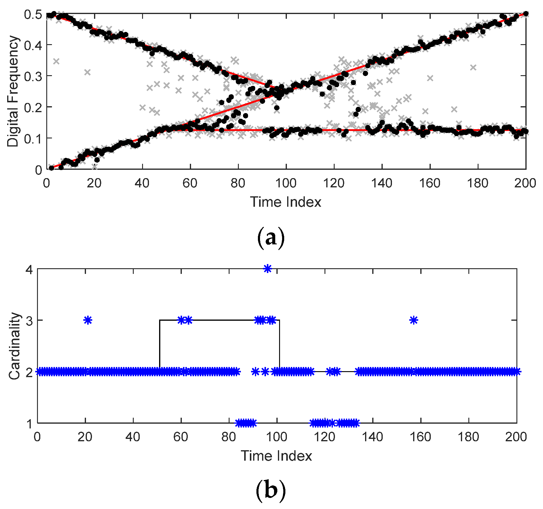
3. SMC-CPHD Filter with Adaptive Survival Probability

The processing steps of the SMC-CPHD filter [23] were reviewed in the previous section. In this section, how to adaptively apply the survival probability is explained, and the result that changing the survival probability does not affect the stability of the filter is demonstrated through convergence analysis.

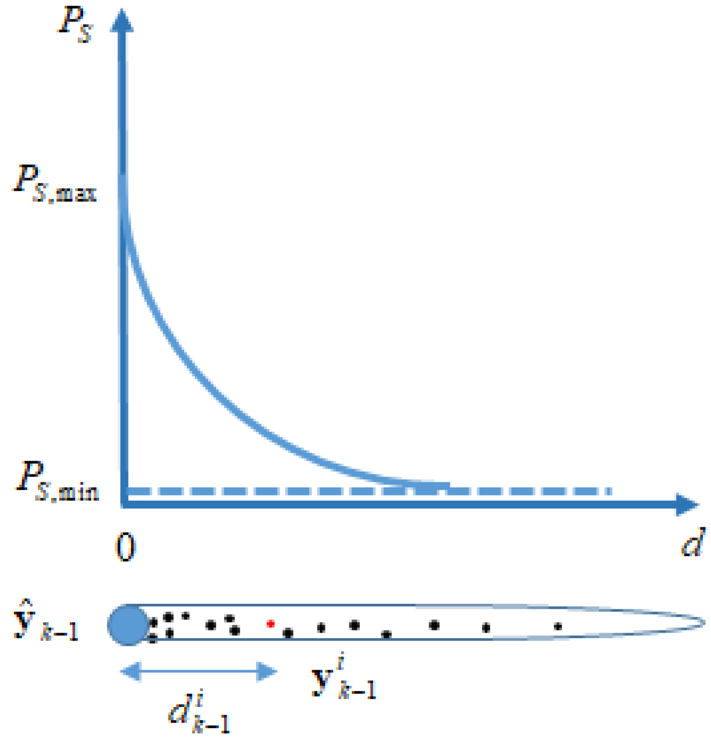
3.1. New Adaptive Survival Probability

As mentioned previously, the existing versions of the SMC-CPHD filter employ a predesigned value for the survival probability, which remains identical for all targets independent of distances between their posterior estimate and particles [7,8,10,23]. Here, we describe a simple survival model shown by p S , k | k 1 ( y k 1 i ) p S ( y k 1 i ) to adaptively compute the survival probability of the state variable according to the distance from each particle, i = 1 , 2 , , N k 1 .
In the proposed algorithm, the survival model includes a set of the boundary with their corresponding posterior estimate. The probability illustrates the survival probability with respect to the posterior estimate, which is calculated by:
p S ( y k 1 i ) = { p S , max ( i f d k 1 i = 0 ) p S , max exp ( d k 1 i / d max ) ( i f 0 < d k 1 i < d max a n d d M 2 T g ) p S , min = 0.3679 × p S , max ( i f d k 1 i = d max o r d M 2 > T g )
where p S represents the adaptive survival probability at time k , p S , m a x represents the maximum value of p S , and exp ( ) is the exponential function. p S , min indicates the minimum value of p S and is equal to 0.3679 × p S , m a x because exp ( 1 ) = 0.3679 in the case of d k 1 i = d max , with d max being the maximum distance of a particle to the prior. d k 1 i = | y k 1 i y ^ k 1 | denotes the Euclidean distance between the posterior estimate, y ^ k 1 , and the i -th of each particle y k 1 i at time k , d m a x is the maximum value of the distance, d k 1 i , and y ^ k 1 is the observation location. d M 2 ( ε k ( i j ) ) T ( P z , k | k 1 ( j ) ) 1 ε k ( i j ) is the Mahalanobis distance associated with ε k ( i j ) and d M 2 T g represents the validation gate area, which is selected to reduce false but apparently possible target measurements in the presence of the clutter or noise [28,29,30,31,32]. The other related notations are as follows: ε k ( i j ) z k ( i ) h ( y k | k 1 ( j ) ) denotes the innovation vector associated with the i -th measurement, z k ( i ) Z k , and with respect to that, the j -th predicted observation, P ε , k | k 1 ( j ) = P z , k | k 1 ( j ) = H P y , k | k 1 ( j ) H T + R is the residual covariance matrix of ε k ( i j ) , R defines the measurement noise covariance matrix, h ( y k | k 1 ( j ) ) refers to the measurement model, and T g is the threshold of the n y -dimensional validation gate and a design parameter.
Figure 1 shows the adaptive survival probability based on (23).
As shown in Figure 1, the closer the distance, d k 1 i , the higher the probability of survival. As mentioned previously and shown in (23), the adaptive survival probability, p S , does not consist of constant values but varying values according to the distance within a validation gate area, and p S , min is not zero but a value determining by p S , max . The parameter p S , max is a design parameter and is set to 1 in our simulations. In the setting of the value of p S , max , the value of 0.98 is often used for the fixed survival probability [23], while the value of one is used for consideration of the attenuation of the survival probability according to the distance [24].
However, an improvement of the proposed method is still needed. When we apply the calculated value d max to set the survival probability, the sample impoverishment can occur in the worst case because the survival probability is directly affected by the distance. Therefore, an additional method such as distance leveling for obtaining enough samples may be necessary. Nevertheless, the proposed method is meaningful because the effect of resampling in the SMC-CPHD filter can be present; p S has an effect on the weights of the particles because p S is multiplied to the weights of the particles. Simulations for verifying the performance improvement of the proposed algorithm are shown in Section 5.

3.2. Convergence Analysis

The bounds for the mean square error (MSE) [33,34] of the SMC-PHD filter depend on some considerations related to the designed parameters of the model of the target system. In order to verify the convergence of the proposed algorithm, those analysis results are extended and applied to the proposed algorithm. In particular, the effect of the character that changed the survival probability in Section 3.1 on the convergence of the filter is analyzed. Some of the assumptions and considerations used in the convergence analysis are given as follows.
If θ N defines a sequence of measures that rely on the number of particles, N , then θ N converges to θ when φ B ( R d ) .
lim N E [ ( θ N , φ θ , φ ) 2 ] = 0
where B ( R d ) denotes the set of bounded Borel measurable function on R d and d refers to the dimension of the space. When the measure in the inner product, . , . , is discrete, it is the summation inner product:
D k | k N , φ = i = 1 N w k ( i ) φ ( x k ( i ) )
In order to prove convergence of the proposed algorithm, D k | k 1 is defined as the density propagated from the previous time step, and the boundary of | D k | k N , φ D k | k 1 , φ | is analyzed by the triangle inequality:
| D k | k 1 N , φ D k | k 1 , φ | | D k | k 1 N , φ D k 1 | k 1 N , π k | k 1 φ | + | D k 1 | k 1 N , π k | k 1 φ D k 1 | k 1 , π k | k 1 φ |
where π k | k 1 refers to the transition density and is bounded by the system transition, f k | k 1 , and the PHD of spawned targets, s k | k 1 , as follows:
π k | k 1 ( y , y k 1 ) = p S ( y k 1 ) f k | k 1 ( y | y k 1 ) + s k | k 1 ( y | y k 1 )
Let ς k 1 be the σ -algebra generated by the particles { y k 1 ( i ) } . Then, the first term of the right side of (26) can be expected as:
E [ ( D k | k 1 N , φ D k 1 | k 1 N , π k | k 1 φ ) 2 | ς k 1 ] = E [ D k | k 1 N , φ 2 ] D k 1 | k 1 N , π k | k 1 φ 2
The above equation can be expressed in sum using the independence of each particle as follows:
E [ D k | k 1 N , φ 2 ] D k 1 | k 1 N , π k | k 1 φ 2 = ( T ^ N ) 2 i = 1 N ( E [ ( φ ( y ˜ k ( i ) ) p s ( y k 1 ) ) 2 | ς k 1 ] ( π k | k 1 φ ) ( y k 1 ( i ) ) 2 )
where T ^ denotes the estimated number of targets.
According to (29), the equation’s boundary can be expressed as:
| E [ D k | k 1 N , φ 2 ] D k 1 | k 1 N , π k | k 1 φ 2 | T ^ 2 N φ 2 ( p s ( y k 1 ) 2 + π k | k 1 2 )
Using the inequality of Minkowski, (30) can be rearranged as:
E [ ( D k | k 1 N , φ D k | k 1 , φ ) 2 ] 1 / 2 E [ ( D k | k 1 N , φ D k 1 | k 1 N , π k | k 1 φ ) 2 ] 1 / 2 + E [ ( D k 1 | k 1 N , π k | k 1 φ D k 1 | k 1 , π k | k 1 φ ) 2 ] 1 / 2
If there are no newly created targets at time k , the boundary of (31) can be finally expressed as:
E [ ( D k | k 1 N , φ D k | k 1 , φ ) 2 ] 1 / 2 1 N φ ( T ^ p s ( x k 1 ) 2 + π k | k 1 2 ) 1 / 2 + c k 1 | k 1
In (32), c k 1 | k 1 defines the MSE’s boundary at the previous time step, k 1 , and can be obtained from the assumption that:
E [ ( D k 1 | k 1 N , φ D k 1 | k 1 , φ ) 2 ] c k 1 | k 1 φ 2 N
Finally, if π k | k 1 1 + T k | k 1 , where T k | k 1 denotes the number of spawned targets at time step k :
E [ ( D k | k 1 N , φ D k | k 1 , φ ) 2 ] φ 2 N ( ( T ^ p s ( y k 1 ) 2 + 1 + T k | k 1 2 ) 1 / 2 + c k 1 | k 1 ) 2
In the case of the proposed algorithm, we confirmed that the MSE’s convergence depends on only the number of targets, T ^ , including the spawned targets, T k | k 1 , the particles’ number, N , and the maximum boundary of the survival probability. Thus, if the maximum range of the survival probability is specified ( p s , max ), as in the previous section, the SMC-CPHD filter will converge as φ 2 N ( ( T ^ p s , max 2 + 1 + T k | k 1 2 ) 1 / 2 + c k 1 | k 1 ) 2 .

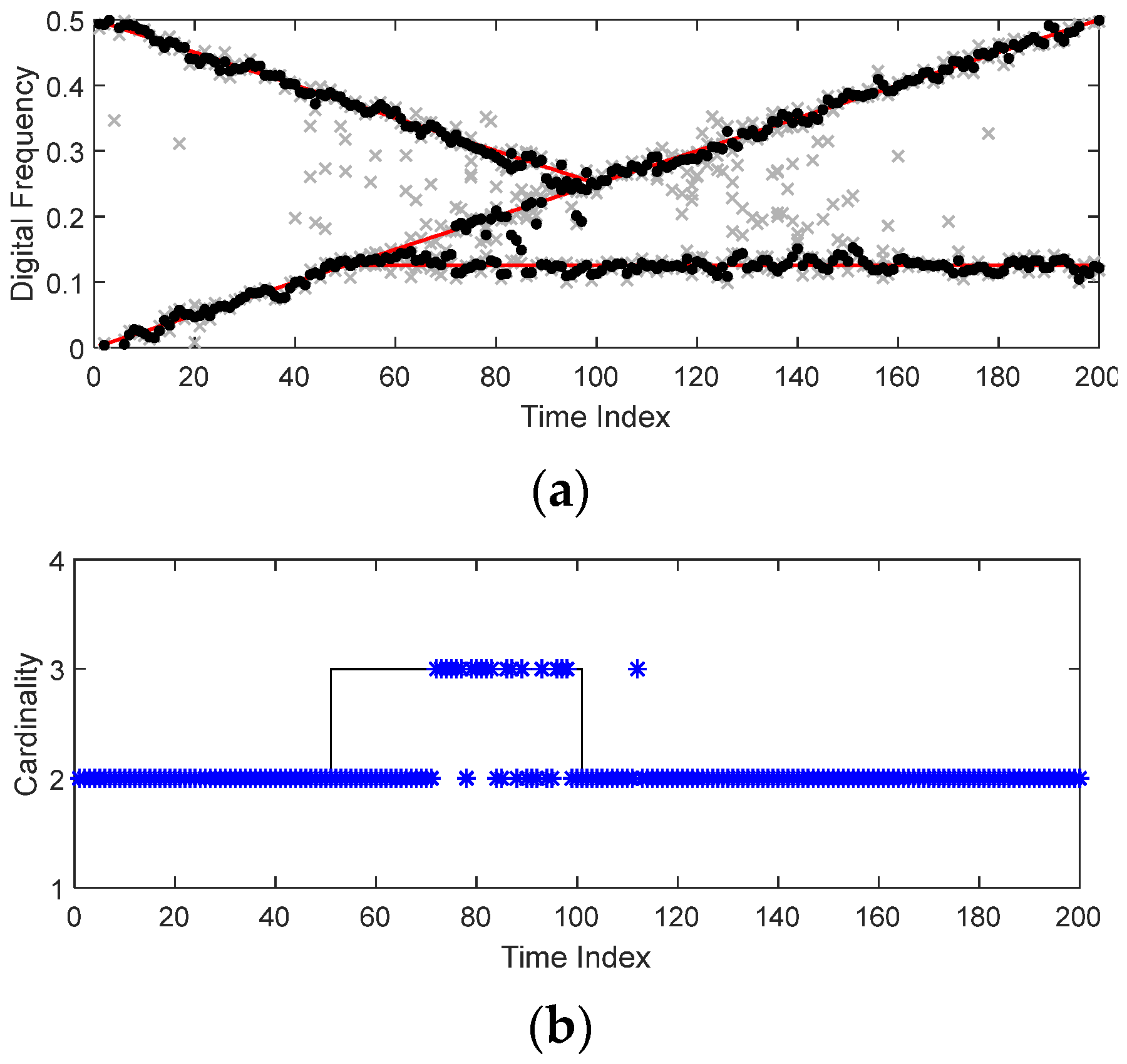
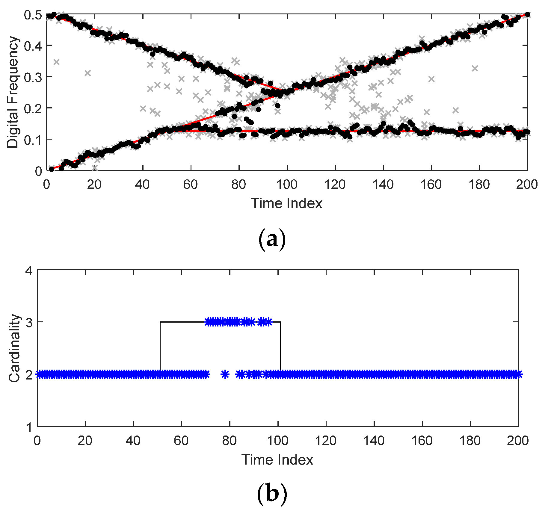
4. Cardinality Compensation with ICI
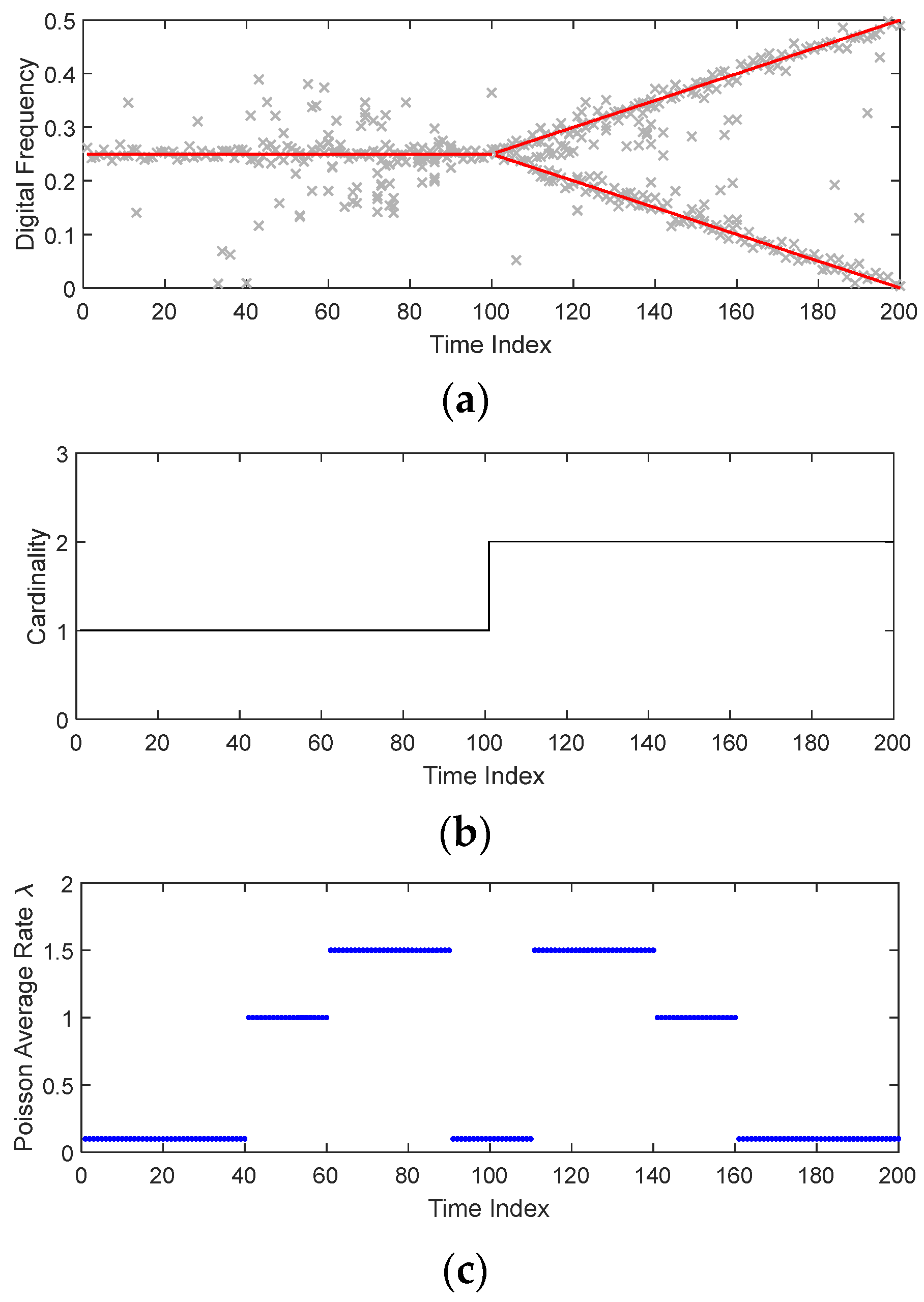
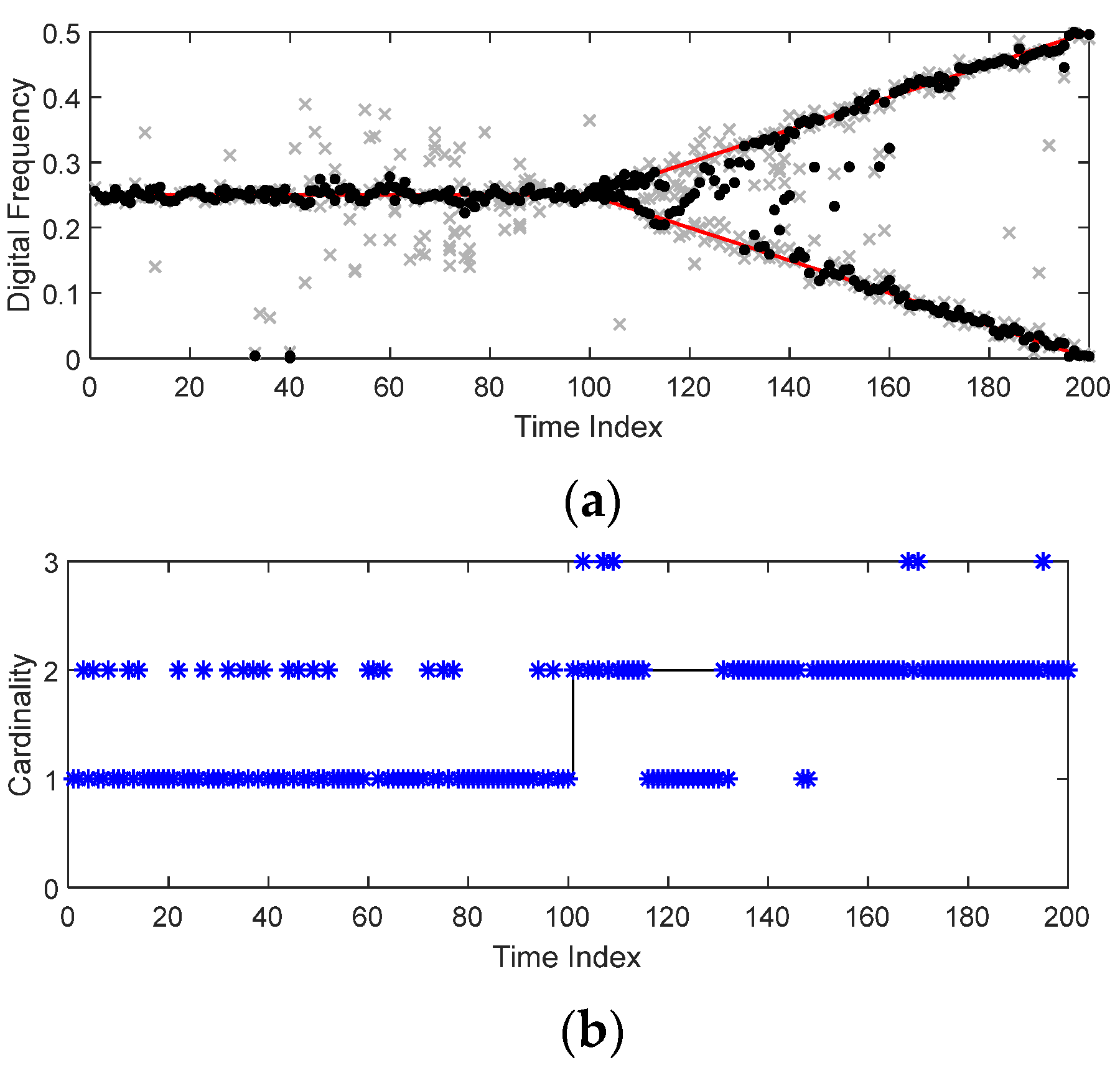
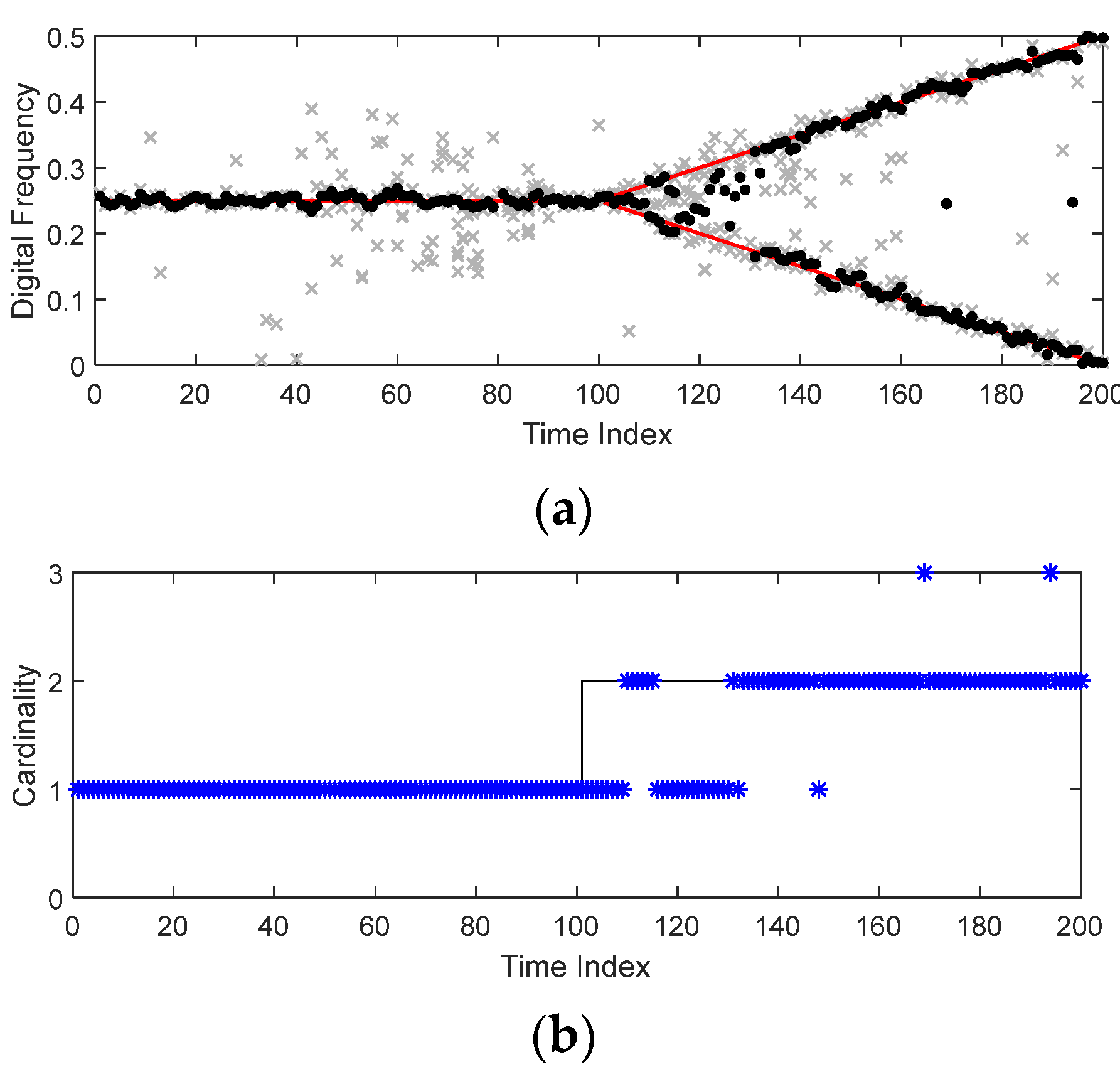
Information fusion is mainly applied to combine information using various sensors in the sensor fusion field. Typical methods, such as CI, cross covariance, sequential CI, and ellipsoidal intersection methods [26,27,35,36,37,38], have been consistently studied. They are classified as ellipsoidal methods and the ICI method [26,27], which is one of the latest data fusion methods. A data fusion method based on the ICI is proposed to obtain less conservative but still consistent estimates. A major advantage of the ICI method is that its fusion results are more accurate than those of the CI method [27]. Therefore, the ICI method is used for combining two pieces of cardinality information.
According to fusion methods, the cardinality, C f , can be determined as:
C f = α C 1 + β C 2
for any γ [ 0 , 1 ] . The covariance of the fused cardinality and gains in (35) are set as α = P C f × ( ( P C 1 ) 1 γ ( γ P C 1 + ( 1 γ ) P C 2 ) 1 ) and β = P C f × ( ( P C 1 ) 1 ( 1 γ ) ( γ P C 1 + ( 1 γ ) P C 2 ) 1 ) . C 1 is the estimated cardinality using the CPHD filter, and P C 1 is the variance of C 1 . C 2 is the additionally generated cardinality by iterative clustering to compensate for the original cardinality estimate, C 1 . The iterative clustering algorithm [39] repeatedly performs fuzzy c-means (FCM) clustering using the resampled particles obtained from the CPHD filter. The clustering number that maximizes the clustering evaluation index among the candidates of the clustering number is selected as cardinality information, C 2 . P C 2 defines the quality information and represents the variance of C 2 . Finally, the covariance of the fused cardinality can be calculated by:
( P C f ) 1 = ( P C 1 ) 1 + ( P C 2 ) 1 ( γ P C 1 + ( 1 γ ) P C 2 ) 1
The compensation method using the ICI method does not always guarantee good performance before fusing. A certain condition is required to continuously obtain the well-fused results and is analyzed by an inequality equation. Because the cardinality is a scalar value, Equation (36) can be expressed as:
1 P C f 1 P C 1 = 1 P C 2 1 γ P C 1 + ( 1 γ ) P C 2
If the difference in Equation (37) is positive, the fused result using the ICI method always has better estimated results compared with those of the CPHD filter. Therefore, to always make the above equation positive, the γ P C 1 + ( 1 γ ) P C 2 term guarantees the positive condition or is equal to zero. The term is multiplied in both sides of (37) and is then rewritten as follows:
( 1 P C f 1 P C 1 ) × ( γ P C 1 + ( 1 γ ) P C 2 ) = ( 1 P C 2 1 γ P C 1 + ( 1 γ ) P C 2 ) × ( γ P C 1 + ( 1 γ ) P C 2 ) = γ ( P C 1 P C 2 1 )
where γ [ 0 , 1 ] . In addition, if P C 1 P C 2 , γ ( P C 1 P C 2 1 ) 0 . This means that the fused result with the ICI method has a lower estimated error compared with the original CPHD filter. Finally, the estimated cardinality is only used in the P C 1 P C 2 case when performing the ICI-based cardinality compensation process.

5. Simulations

Simulations were performed to verify the performance of the proposed algorithm. This paper aims to track multiple frequencies using the CPHD filter to remove GNSS interference when GNSS signals are received with multiple GNSS interference signals.
In each simulation, GNSS data were generated by a SatGen simulator. The frequencies of received GNSS interference signals were designed as the combination of a constant frequency and a linear changed frequency in the time-frequency domain. We simulated two cases, and the true values of trajectory including the cardinality of each case are shown in Figure 2 and Figure 3. In Figure 2a and Figure 3a, the solid red line indicates the true trajectory, and the gray crosses show the frequency measurement, including the clutter of the CPHD filter. In both cases, the clutter conditions were set differently, as shown in Figure 2c, to confirm how resistant the proposed method is to the clutter. The jamming to signal ratio was set to 30 dB, the power of the received GNSS signal was set to −130 dBm, and the overall noise floor was set to −114 dB/MHz. In addition, the chirp rate was set to 3.65 × 10 12 Hz / s [40,41]. The initial digital frequency was set to 0.25 in case 1 and was respectively set to 0 and 0.5 in case 2. The intermediate frequency was 9.548 MHz, and the sampling frequency was 38.192 MHz.
The A_CPHD was compared with the following methods: The first method is “C_CPHD”, which is a conventional CPHD filter with k-means clustering. The second method is “FCM_CPHD”, which is a conventional CPHD filter applying FCM clustering so that it is robust in the presence of heavy noise and clutter. The last method is “CC_CPHD”, which is the FCM_CPHD applying cardinality compensation [22] with the ICI method and iterative clustering, which was recently proposed.
In the first and second cases, the tracking and cardinality estimate results from each method are presented as shown in Figure 4, Figure 5, Figure 6, Figure 7, Figure 8, Figure 9, Figure 10 and Figure 11. The top panel of each figure indicates the frequency tracking result, and the bottom panel of each figure shows the cardinality estimate result. In each top graph, the true trajectory is indicated by the solid red line, the measurements with the clutter are shown by the gray crosses, and the black dots present the estimation results. In each bottom graph, the estimation result of cardinality is shown in the solid black line, and the true value of cardinality is presented by the solid black line. As shown in Figure 2c, the distribution of clutter varies with time. The clutter had the Poisson distribution property. Here, the Poisson average rate value ( λ ) in the frequency measurement was changed over a total of 300 simulation runs.
In Figure 4, the C_CPHD was used. As shown in this figure, tracking loss partially occurs, and the cardinality error was also severe. The results of FCM_CPHD are shown in Figure 5. Through these results, we confirmed that the tracking performance of the FCM_CPHD was a little better than that of the C_CPHD due to the robustness of the clustering method when there is a lot of noise in the measurement.
However, there was still tracking loss, and estimated errors of cardinality still remained even though FCM clustering was used. Therefore, we proposed the cardinality compensation method to improve the tracking performance. According to Figure 6, the performance of the frequency tracking and the cardinality estimate were ameliorated when the CC_CPHD was used.
However, as shown in Figure 6b, the true value of cardinality is 2 when the time index is 165, but the estimated value is 3. We eventually aim to eliminate the frequency of the interference signal by using the estimation result as the notch frequency. Therefore, the problem arises of increasing the dimension of the notch filter if the number of the frequency to be removed is estimated to be more than the true number. In addition, as shown in Figure 6a, a performance improvement of the algorithm is needed to prevent this situation because this is a result of estimating the wrong frequencies, resulting in the elimination of frequency components that should not be removed. Therefore, we have proposed the adaptive survival probability as earlier described, and the results are shown in Figure 7.
The results in Figure 7 show that the estimated results of both frequency and cardinality represent close to the true value. The cardinality value differs from the true value when the time index is from 101 to 109, as seen in Figure 7b, because the distance between the two frequencies at that time is too close, meaning that the estimate accuracy is reduced.
To evaluate the tracking performance, an optimal sub-pattern assignment (OSPA) [42], which is a general performance index used in the multiple target tracking field, was used as a performance index.
Table 1 shows the results from Figure 4, Figure 5, Figure 6 and Figure 7 by the OSPA index, and the proposed method with adaptive survival probability (A_CPHD) has a small OSPA index compared to the existing methods. This means that the estimate performance of frequency and cardinality was improved. The improvement of the computational efficiency was also found through a smaller calculation time than the CC_CPHD without adaptive survival probability. These results can be considered as the effect of adaptive gating due to applying the probability by the conditions.
The second simulation assumes that more complex multiple frequencies are input than the first simulation case, as shown in Figure 3. The clutter conditions are the same as in case 1. Figure 8, Figure 9, Figure 10 and Figure 11 show the results of estimating frequency and cardinality for case 2 using the C_CPHD, FCM_CPHD, CC_CPHD, and A_CPHD methods, respectively. Table 2 shows the results in Figure 8, Figure 9, Figure 10 and Figure 11 by the OSPA performance index. As shown in Figure 8, Figure 9, Figure 10 and Figure 11 and Table 2, the performance of the proposed algorithm for case 2, like case 1, is superior to that of the existing methods. However, in the second scenario, the OSPA of the FCM_CPHD is not significantly improved compared with the results of C_CPHD, unlike the first scenario, which results from a strong tendency to unite in one when clustering by FCM in cases where the frequencies are dense. In addition, for CC_CPHD and A_CPHD using the iterative clustering method, the calculation time in the first scenario is twice as much as C_CPHD and FCM_CPHD, while the second scenario is tripled. This is because the number of targets (frequencies) to estimate increased, and the number of candidates for iterative clustering consequently increased, which results from increasing the calculation time.
From the simulation results for both cases, the combination of FCM and cardinality compensation methods (CC_CPHD) shows a significant improvement in performance over existing methods. However, depending on the scenarios and the degree of the clutter, the estimated cardinality may be more than the actual cardinality, as in Figure 6b and Figure 10b. From the perspective of ultimately eliminating frequencies, as mentioned briefly previously, the mitigation performance can be degraded because the number of frequencies to be removed is increased; thus it is hard to respond to this situation. However, the addition of the proposed adaptive survival probability shows more robust performance in the clutter or scenarios.
Consequently, through the above simulation results, we confirmed that the proposed adaptive survival probability is effective in improving performance compared to constant survival probability under any clutter conditions. This was because survival probability affected the weight of the particles, resulting in an adaptive gating effect. However, a review of the resampling methods may be necessary because sample impoverishment may occur if the adaptive boundary is incorrectly set.

6. Conclusions

We proposed an SMC-CPHD filter with adaptive survival probability for multiple frequency tracking to enhance the tracking performance in the conventional SMC-CPHD filter. The survival probability of the particles in the filter was adjusted using the pre-designed exponential function. In order to confirm whether the proposed survival probability affects the stability of the filter, the error bounds in the prediction process were analyzed. Moreover, the ICI based compensation technique was added to improve cardinality tracking performance. To evaluate the proposed method’s performance, MATLAB-based simulations were performed. As a result, we confirmed that the tracking performance of the multiple frequencies and the accuracy of cardinality estimates were improved compared to the existing filters.

Author Contributions

Conceptualization, S.Y.K.; methodology, S.Y.K.; validation, S.Y.K. and C.H.K.; formal analysis, S.Y.K. and C.H.K.; investigation, S.Y.K.; writing—original draft preparation, S.Y.K.; writing—review and editing, S.Y.K. and C.H.K.; visualization, S.Y.K.; supervision, C.H.K. and C.G.P.; funding acquisition, C.G.P. All authors have read and agreed to the published version of the manuscript.

Funding

This work was supported by AI-based Flight Control Research Laboratory funded by the Defense Acquisition Program Administration under Grant UD200045CD.

Institutional Review Board Statement

Not applicable.

Informed Consent Statement

Not applicable.

Data Availability Statement

Not applicable.

Conflicts of Interest

The authors declare no conflict of interest.

References

  1. Fortmann, T.; Bar-Shalom, Y.; Scheffe, M. Sonar tracking of multiple targets using joint probabilistic data association. IEEE J. Ocean. Eng. 1983, 8, 173–184. [Google Scholar]
  2. Bar-Shalom, Y.; Fortmann, T. Tracking and Data Association; Academic Press: Boston, MA, USA, 1988. [Google Scholar]
  3. Blackman, S.; Popoli, R. Design and Analysis of Modern Tracking Systems; Artech House: Boston, MA, USA, 1999. [Google Scholar]
  4. Mahler, R.P. Multitarget Bayes filtering via first-order multitarget moments. IEEE Trans. Aerosp. Electron. Syst. 2003, 39, 1152–1178. [Google Scholar] [CrossRef]
  5. Blackman, S.S. Multiple hypothesis tracking for multiple target tracking. IEEE Aerosp. Electron. Syst. Mag. 2004, 19, 5–18. [Google Scholar]
  6. Vo, B.N.; Singh, S.; Doucet, A. Sequential Monte Carlo methods for multitarget filtering with random finite sets. IEEE Trans. Aerosp. Electron. Syst. 2005, 41, 1224–1245. [Google Scholar]
  7. Vo, B.N.; Ma, W.K. The Gaussian mixture probability hypothesis density filter. IEEE Trans. Signal Process. 2006, 54, 4091–4104. [Google Scholar] [CrossRef]
  8. Mahler, R.P. Statistical Multisource-Multitarget Information Fusion; Artech House: Boston, MA, USA, 2007. [Google Scholar]
  9. Mahler, R. PHD filters of higher order in target number. IEEE Trans. Aerosp. Electron. Syst. 2007, 43, 1523–1543. [Google Scholar] [CrossRef]
  10. Vo, B.T.; Vo, B.N.; Cantoni, A. Analytic implementations of the cardinalized probability hypothesis density filter. IEEE Trans. Signal Process. 2007, 55, 3553–3567. [Google Scholar]
  11. Fu, Z.; Feng, P.; Angelini, F.; Chambers, J.; Naqvi, S.M. Particle PHD filter based multiple human tracking using online group-structured dictionary learning. IEEE Access 2018, 6, 14764–14778. [Google Scholar] [CrossRef]
  12. Hosseini, S.S.; Jamali, M.M.; Särkkä, S. Variational Bayesian adaptation of noise covariances in multiple target tracking problems. Measurement 2018, 122, 14–19. [Google Scholar]
  13. Bao, Z.; Jiang, Q.; Liu, F. A PHD Based Particle Filter for Detecting and Tracking Multiple Weak Targets. IEEE Access 2019, 7, 145843–145850. [Google Scholar] [CrossRef]
  14. Clark, D.; Ruiz, I.T.; Petillot, Y.; Bell, J. Particle PHD filter multiple target tracking in sonar image. IEEE Trans. Aerosp. Electron. Syst. 2007, 43, 409–416. [Google Scholar] [CrossRef]
  15. Pham, N.T.; Huang, W.; Ong, S.H. Tracking multiple objects using probability hypothesis density filter and color measurements. In Proceedings of the 2007 IEEE International Conference on Multimedia and Expo, Beijing, China, 2–5 July 2007; pp. 1511–1514. [Google Scholar]
  16. Maggio, E.; Taj, M.; Cavallaro, A. Efficient multitarget visual tracking using random finite sets. IEEE Trans. Circuits Syst. Video Technol. 2008, 18, 1016–1027. [Google Scholar] [CrossRef] [Green Version]
  17. Battistelli, G.; Chisci, L.; Morrocchi, S.; Papi, F.; Benavoli, A.; Farina, A.; Graziano, A. Traffic intensity estimation via PHD filtering. In Proceedings of the 2008 European Radar Conference, Amsterdam, The Netherlands, 30–31 October 2008; pp. 340–343. [Google Scholar]
  18. Juang, R.R.; Levchenko, A.; Burlina, P. Tracking cell motion using GM-PHD. In Proceedings of the 2009 IEEE International Symposium on Biomedical Imaging: From Nano to Macro, Boston, MA, USA, 28 June–1 July 2009; pp. 1154–1157. [Google Scholar]
  19. Pollard, E.; Plyer, A.; Pannetier, B.; Champagnat, F.; Le Besnerais, G. GM-PHD filters for multi-object tracking in uncalibrated aerial videos. In Proceedings of the 12th International Conference on Information Fusion, Seattle, WA, USA, 6–9 July 2009; pp. 1171–1178. [Google Scholar]
  20. Ulmke, M.; Erdinc, O.; Willett, P. GMTI tracking via the Gaussian mixture cardinalized probability hypothesis density filter. IEEE Trans. Aerosp. Electron. Syst. 2010, 46, 1821–1833. [Google Scholar] [CrossRef]
  21. Mullane, J.; Vo, B.N.; Adams, M.D.; Vo, B.T. A random-finite-set approach to Bayesian SLAM. IEEE Trans. Robot. 2011, 27, 268–282. [Google Scholar] [CrossRef]
  22. Kim, S.Y. Multiple frequency tracking method based on the cardinalised probability hypothesis density filter with cardinality compensation. In Proceedings of the 31st International Technical Meeting of the Satellite Division of The Institute of Navigation (ION GNSS+ 2018), Miami, FL, USA, 24–28 September 2018; pp. 3504–3517. [Google Scholar]
  23. Ristic, B.; Clark, D.; Vo, B.N.; Vo, B.T. Adaptive target birth intensity for PHD and CPHD filters. IEEE Trans. Aerosp. Electron. Syst. 2012, 48, 1656–1668. [Google Scholar] [CrossRef]
  24. Yazdian-Dehkordi, M.; Azimifar, Z. Refined GM-PHD tracker for tracking targets in possible subsequent missed detections. Signal Process. 2015, 116, 112–126. [Google Scholar] [CrossRef]
  25. Chen, X.; Li, Y.; Yu, J. PHD and CPHD Algorithms Based on a Novel Detection Probability Applied in an Active Sonar Tracking System. Appl. Sci. 2018, 8, 36. [Google Scholar] [CrossRef] [Green Version]
  26. Sijs, J.; Lazar, M. State fusion with unknown correlation: Ellipsoidal intersection. Automatica 2012, 48, 1874–1878. [Google Scholar] [CrossRef] [Green Version]
  27. Noack, B.; Sijs, J.; Reinhardt, M.; Hanebeck, U.D. Decentralized data fusion with inverse covariance intersection. Automatica 2017, 79, 35–41. [Google Scholar] [CrossRef]
  28. Gordon, N.; Ristic, B.; Arulampalam, S. Beyond the Kalman Filter: Particle Filters for Tracking Applications; Artech House: London, UK, 2004. [Google Scholar]
  29. Zhang, H.; Jing, Z.; Hu, S. Gaussian mixture CPHD filter with gating technique. Signal Process. 2009, 89, 1521–1530. [Google Scholar] [CrossRef]
  30. Macagnano, D.; de Abreu, G.T.F. Adaptive gating for multitarget tracking with Gaussian mixture filters. IEEE Trans. Signal Process. 2012, 60, 1533–1538. [Google Scholar] [CrossRef]
  31. Cheng, T.; Li, X.R.; He, Z. Comparison of gating techniques for maneuvering target tracking in clutter. In Proceedings of the 17th International Conference on Information Fusion, Salamanca, Spain, 7–10 July 2014; pp. 1–8. [Google Scholar]
  32. Si, W.; Wang, L.; Qu, Z. Multi-target tracking using an improved Gaussian mixture CPHD Filter. Sensors 2016, 16, 1964. [Google Scholar] [CrossRef] [PubMed] [Green Version]
  33. Clark, D.E.; Bell, J. Convergence results for the particle PHD filter. IEEE Trans. Signal Process. 2006, 54, 2652–2661. [Google Scholar]
  34. Johansen, A.M.; Singh, S.S.; Doucet, A.; Vo, B.N. Convergence of the SMC Implementation of the PHD Filte. Methodol. Comput. Appl. Probab. 2006, 8, 265–291. [Google Scholar] [CrossRef] [Green Version]
  35. Zarei-Jalalabadi, M.; Malaek, S.M.B. Practical method to predict an upper bound for minimum variance track-to-track fusion. IET Signal Process. 2017, 11, 961–968. [Google Scholar] [CrossRef]
  36. Niehsen, W. Information fusion based on fast covariance intersection filtering. In Proceedings of the 5th International Conference on Information Fusion, Annapolis, MD, USA, 8–11 July 2002; pp. 901–904. [Google Scholar]
  37. Deng, Z.; Zhang, P.; Qi, W.; Liu, J.; Gao, Y. Sequential covariance intersection fusion Kalman filter. Inf. Sci. 2012, 189, 293–309. [Google Scholar] [CrossRef]
  38. Li, W.; Wang, Z.; Wei, G.; Ma, L.; Hu, J.; Ding, D. A survey on multisensor fusion and consensus filtering for sensor networks. Discret. Dyn. Nat. Soc. 2015, 2015, 683701. [Google Scholar] [CrossRef] [Green Version]
  39. Kim, S.; Kang, C.; Park, C. Cardinality compensation method based on information-weighted consensus filter using data clustering for multi-target tracking. Chin. J. Aeronaut. 2019, 32, 2164–2173. [Google Scholar] [CrossRef]
  40. Mitch, R.H.; Dougherty, R.C.; Psiaki, M.L.; Powell, S.P.; O’Hanlon, B.W.; Bhatti, J.A.; Humphreys, T.E. Signal Characteristics of Civil GPS Jammers. In Proceedings of the 24th International Technical Meeting of the Satellite Division of the Institute of Navigation (ION GNSS 2011), Portland, Oregon, 19–23 September 2001; pp. 1907–1919. [Google Scholar]
  41. Mitch, R.H.; Psiaki, M.L.; O’Hanlon, B.W.; Powell, S.P.; Bhatti, J.A. Civilian GPS Jammer Signal Tracking and Geolocation. In Proceedings of the 25th International Technical Meeting of the Satellite Division of the Institute of Navigation (ION GNSS 2012), Nashville, TN, USA, 17–21 September 2012; pp. 2901–2920. [Google Scholar]
  42. Schuhmacher, D.; Vo, B.T.; Vo, B.N. A consistent metric for performance evaluation of multi-object filters. IEEE Trans. Signal Process. 2008, 56, 3447–3457. [Google Scholar] [CrossRef] [Green Version]
Figure 1. The adaptive survival probability.
Applsci 12 01369 g001
Figure 2. True trajectory (case 1): (a) Measurement and clutter; (b) Cardinality; (c) The Poisson average rate of clutter according to time index.
Applsci 12 01369 g002
Figure 3. True trajectory (case 2): (a) Measurement and clutter; (b) Cardinality.
Applsci 12 01369 g003
Figure 4. The result of the C_CPHD (case 1): (a) Frequency tracking; (b) Cardinality estimate.
Applsci 12 01369 g004
Figure 5. The result of the FCM_CPHD (case 1): (a) Frequency tracking; (b) Cardinality estimate.
Applsci 12 01369 g005
Figure 6. The result of the CC_CPHD (case 1): (a) Frequency tracking; (b) Cardinality estimate.
Applsci 12 01369 g006
Figure 7. The result of the A_CPHD (case 1): (a) Frequency tracking; (b) Cardinality estimate.
Applsci 12 01369 g007
Figure 8. The result of the C_CPHD (case 2): (a) Frequency tracking; (b) Cardinality estimate.
Applsci 12 01369 g008
Figure 9. The result of the FCM_CPHD (case 2): (a) Frequency tracking; (b) Cardinality estimate.
Applsci 12 01369 g009
Figure 10. The result of the CC_CPHD (case 2): (a) Frequency tracking; (b) Cardinality estimate.
Applsci 12 01369 g010
Figure 11. The result of the A_CPHD (case 2): (a) Frequency tracking; (b) Cardinality estimate.
Applsci 12 01369 g011
Table 1. The performance of tracking (case 1).
AlgorithmOSPAComputation Time [sec.]
C_CPHD16.23882.6815
FCM_CPHD12.75852.7087
CC_CPHD (without adaptation)6.66674.7724
A_CPHD (Proposed)6.54374.7032
Table 2. The performance of tracking (case 2).
AlgorithmOSPAComputation Time [sec.]
C_CPHD17.22843.5796
FCM_CPHD16.91583.7380
CC_CPHD (without adaptation)7.16349.8984
A_CPHD (Proposed)6.96839.4285
Publisher’s Note: MDPI stays neutral with regard to jurisdictional claims in published maps and institutional affiliations.

