Gaussian Process Surrogates for Modeling Uncertainties in a Use Case of Forging Superalloys

Abstract

The avoidance of scrap and the adherence to tolerances is an important goal in manufacturing. This requires a good engineering understanding of the underlying process. To achieve this, real physical experiments can be conducted. However, they are expensive in time and resources, and can slow down production. A promising way to overcome these drawbacks is process exploration through simulation, where the finite element method (FEM) is a well-established and robust simulation method. While FEM simulation can provide high-resolution results, it requires extensive computing resources to do so. In addition, the simulation design often depends on unknown process properties. To circumvent these drawbacks, we present a Gaussian Process surrogate model approach that accounts for real physical manufacturing process uncertainties and acts as a substitute for expensive FEM simulation, resulting in a fast and robust method that adequately depicts reality. We demonstrate that active learning can be easily applied with our surrogate model to improve computational resources. On top of that, we present a novel optimization method that treats aleatoric and epistemic uncertainties separately, allowing for greater flexibility in solving inverse problems. We evaluate our model using a typical manufacturing use case, the preforming of an Inconel 625 superalloy billet on a forging press.

1. Introduction

Conducting experiments to better understand manufacturing processes is crucial, with real physical experiments being considered the gold standard. However, conducting real physical experiments for each new experimental setting is impractical because of expensive materials, production stoppages and labor hours for monitoring and evaluation. One good alternative is conducting experiments via simulation, where numerical methods–such as Finite Element Method (FEM)–present a well-observed method in the field of structural analysis. However, solving complex problems with FEM is time-consuming and computationally expensive. In order to reduce the computational effort, surrogate modeling may offer a promising solution [1]. Surrogate models are trained in a supervised manner and are designed to learn the function mapping between inputs and outputs. With a sufficient amount of training data with respect to the observed use case, a customized surrogate model is able to substitute for a FEM simulation up to a certain accuracy. When only specific dimensions with a controlled reduction in accuracy of a simulation result are desired, reduced-order surrogate modeling is an already known technique. Thus, reduced-order surrogate modeling aims to substitute the high-resolution simulation domain with some carefully selected dimensions of importance, e.g., selected displacement measures of a deformed part can be predicted by a reduced-order surrogate modeling with low computational effort, instead of performing a computationally intensive FEM simulation that predicts the displacement of each node representing the deformed part.

Meanwhile, Gaussian process regression (GP) has been successfully used as a surrogate model in the past. In literature, GP regression is also called “kriging” after the statistician and mining engineer Danie G. Krige [2]. However, for consistency, we use only the term GP regression or plain GP in this paper. Regarding GP regression, one of the biggest advantages is that it predicts a distribution (described by mean and standard deviation) rather than just a point estimate. The predicted standard deviation can be seen as a quality criterion related to the corresponding predicted mean value. In the following, we will refer to that standard deviation of a prediction as epistemic uncertainty, i.e., how certain the model is with respect to its prediction. Considering real manufacturing processes, another source of uncertainty can be observed with regard to the lack of complete control over all influence parameters. These deviations occurring during repeated process iterations under the same conditions are referred to as aleatoric uncertainty.

Recapitulating, we want to shed light on two types of uncertainties in surrogate modeling: (1) epistemic uncertainty referring to the lack of knowledge in respect to a simulation model and can be minimized by adding additional sources of information (with respect to machine learning models, it is mainly increasing the number of training instances at new locations in the feature space) and (2) aleatoric uncertainty referring to deviations of an observed manufacturing process itself, i.e., aleatoric uncertainty cannot be minimized even if more data is generated. Since epistemic and aleatoric uncertainties describe different properties, it seems natural to treat them separately when making predictions or optimization. However, it should be mentioned that in certain circumstances it may be useful to consider uncertainty as a whole rather than dividing it into aleatoric and epistemic uncertainty. In such cases, heteroskedastic GP regression represents a common approach for optimization with surrogate models [3,4,5]. In our problem definition, especially in solving inverse problems, we argue that the distinction of epistemic and aleatoric uncertainty shows clear advantages.

There is a wealth of literature on surrogate models, reduced-order surrogate models, and optimization with GP regression. We present in the following the main related works to our research field organized in (1) GP regression and FEM simulations, (2) GP regression trained with pure sensor data and (3) optimization with GP regression.

In the work of Roberts et al. [6], they predict damage development in forged brake discs reinforced with Al-SiC particles using damage maps. In addition to Multilayer Perceptron (MLP), Roberts et al. [6] utilize GP regression as a surrogate model. Loghin and Ismonov [7] predict the stress intensity factors using GP regression trained with FEM results of a classical bolt-nut assembly use case. Ming et al. [8] model an electrical discharge machining process with GP regression. Su et al. [9] utilize GP regression as a surrogate in a structural reliability analysis of a large suspension bridge. In the work of Guo and Hesthaven [10], GP regression is used as a reduced-order model for nonlinear structural analysis in a 1D and 3D use case, where data generation was performed with active learning. Hu et al. [11] use GP regression to estimate residual stresses field of machined parts from two-dimensional numerical simulations. Yue et al. [12] propose two active learning approaches using GP regression for a composite fuselage use case. In the work of Ortali et al. [13] GP regression is used as a reduced-order surrogate model for fluid dynamics use cases. Venkatraman et al. [14] use GP regression as a surrogate model of texture in micro-springs. GP regression can also be used on data with multiple fidelity levels, where Lee et al. [15] investigate GP regression surrogate modeling with uncertain material properties of soft tissues and multi-fidelity data. Brevault et al. [16] provide an overview of multi-fidelity GP regression techniques in the field of aerospace systems. GP regression can also be extended by methods that stack them or use them in a tree model. Civera et al. [17] predict imperfections in pultruded glass fiber reinforced polymers with a treed method of GP regression trained with experimental data and FEM simulation results. Abdelfatah et al. [18] propose a stacked GP regression to integrate different datasets and propagate uncertainties through the stacked model. GP regression can also be used for calibrating simulations, where Mao et al. [19] use GP regression as a surrogate model in a Bayesian model updating method to calibrate FEM simulation of a long-span suspension bridge.

In addition to the use of FEM data, GP regression also finds application in the use of pure sensor data, which we will discuss in the following. Tapia et al. [20] use a GP regression based surrogate model of a laser powder-bed fusion process to predict melt pool depth. Yu et al. [21] utilize–besides other thriving methods–a GP regression to model the relationship between geological variables and the broken rock zone thickness. Lee [22] uses GP regression trained with experimental data to optimize wire arc additive manufacturing process deposition parameters. Saul et al. [23] propose chained GP regression models based on non-linear latent function combination. Binois et al. [24] provide a heteroskedastic GP regression approach and results of two use cases, namely manufacturing and management of epidemics.

In the course of function maximization with GP regression surrogate models, Dai Nguyen et al. [25] propose a robust optimization approach based on Upper Confidence Bound (UCB) Bayesian Optimization (BO). In another field of optimization, namely solving inverse problems, there is related work found where BO with generalized chi-squared distribution is researched by Huang et al. [26], and Uhrenholt and Jensen [27], where besides standard GP regression Uhrenholt and Jensen [27] utilized warped GP regression from the work of Snelson et al. [28]. An extension of the standard BO can be found in the work of Plock et al. [29], where they combine BO with the Levenberg-Marquardt method. While in maximization and minimization problems aleatoric and epistemic uncertainties can often be treated in the same way, in most cases robust results can be obtained by distinguishing between these two sources of uncertainty [30]. We refer to robust results when mean predictions are associated with low aleatoric uncertainty.

There is already considerable related work in reduced-order surrogate modeling and optimization using GP regression surrogates. However, to the best of our knowledge, we could not identify related work for solving inverse problems in which aleatoric and epistemic uncertainties are treated differently. Optimization approaches for solving inverse problems usually use only epistemic uncertainty. When epistemic and aleatoric uncertainties are taken into account, they are often simply combined, resulting in the potential loss of important information.

To sum up, we identify the following drawbacks:

• Related work shows that mainly epistemic uncertainty is used for prediction or optimization with GP regression.
• In research using aleatoric and epistemic uncertainties, they are not considered separately when solving inverse problems.

As a response, we present the following main contributions of our research to tackle the identified drawbacks of related work:

• We present a GP based surrogate that models (a) the mean result, (b) the aleatoric and (c) the epistemic uncertainty of a manufacturing process outcome.
• We utilize aleatoric and epistemic uncertainties in solving inverse problems for robust optimization results.

With the proposed surrogate model and novel multi-objective optimization strategy, we pave the way for surrogate modeling and inverse problem-solving for practical applications that make use of explicit modeling of sources of uncertainties. Our findings are validated on a typical hot metal forming manufacturing process: preforming an Inconel 625 superalloy billet on a forging press.

This paper is structured as follows. In Section 2, we present the proposed surrogate model, providing an introduction to GP regression in Section 2.1 and describe the GP based parts of our surrogate model in Section 2.2 and Section 2.3. The data generation of aleatoric uncertainty for our surrogate model approach is presented in Section 2.4. Section 3 deals with optimization, where we outline active learning in Section 3.1 and solving inverse problems in Section 3.2. In Section 4 we present the studied use case, preforming an Inconel 625 superalloy billet on a forging press, where we give insights on the design of the forging aggregate characteristics in Section 4.1 and all information regarding the corresponding FEM simulation in Section 4.2. Section 5 shows the results, which are discussed in Section 6. In Section 7, we present the conclusion of our work and an outlook for the future.

2. GP based Surrogate Model

In this section, we first introduce briefly the general idea behind our surrogate modeling approach. We familiarize in Section 2.1 the reader with the general functionality of GP regression to provide an appropriate foundation for the content that follows. In Section 2.2 and Section 2.3 we provide more detailed descriptions of each individual GP of our surrogate model. After describing our surrogate model, we move on to uncertainty propagation analysis with FEM simulation in Section 2.4, where we present the procedure for obtaining aleatoric uncertainties.

GP regression is already well researched for surrogate modeling, replacing expensive target labellers (e.g., numerical simulations, expensive manually labelling, conducting real physical experiments, etc.). One reason is their ability to work with low-dimensional data. Another big advantage of using GP regression is that predictions are made in a probabilistic way, i.e., a prediction is represented by a posterior distribution. Thus, a prediction of GP regression is described by a mean and a covariance. The covariance of a prediction can be used as a metric of prediction confidence, i.e., epistemic uncertainty. We specify that outputs of GP regression describe a distribution with mean m and epistemic uncertainty $\sigma$.

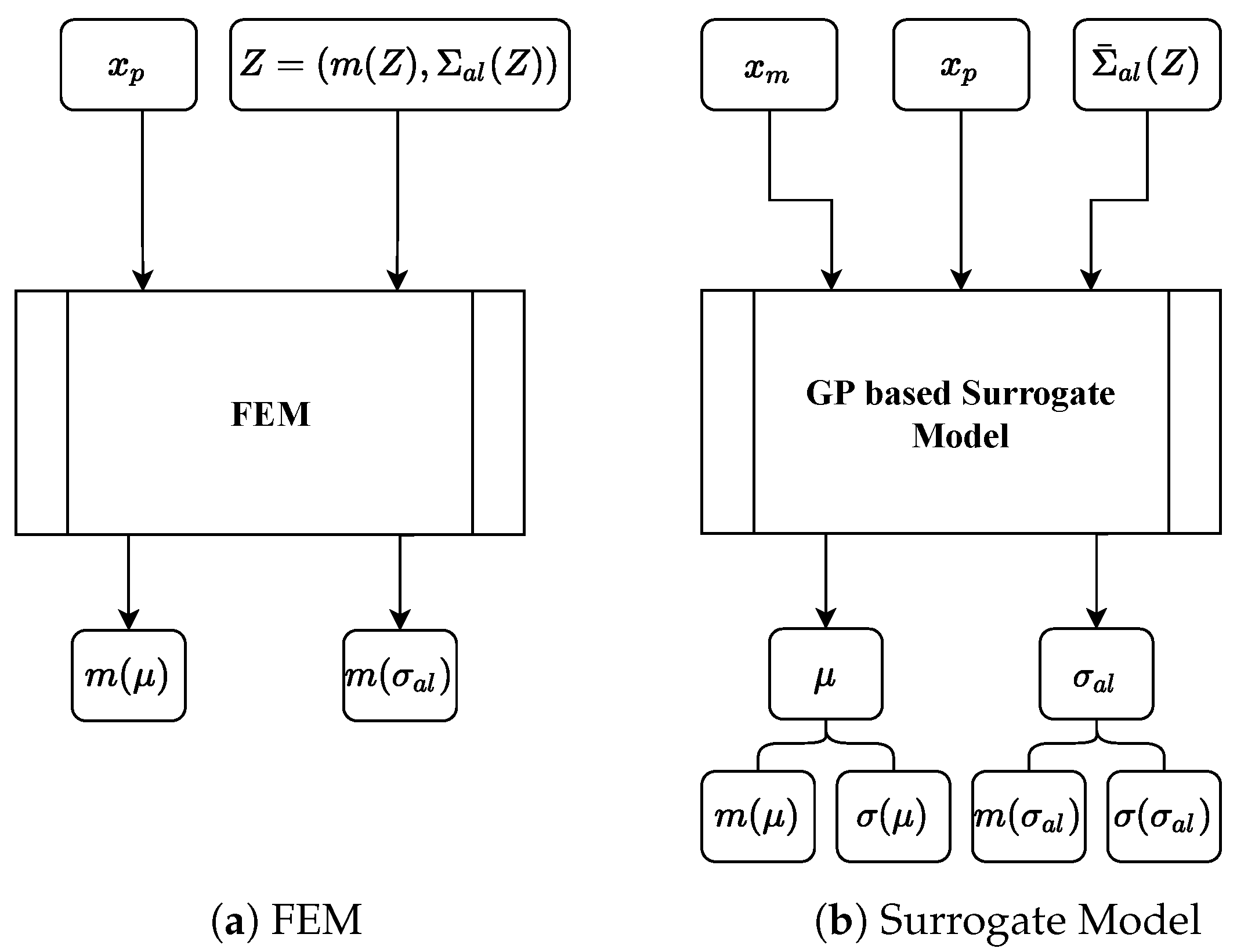
The proposed surrogate model consists of two individual GPs and takes manufacturing process-specific parameters $x_m$, part-specific parameters $x_p$ and aleatoric process uncertainty ${\overline{\mathsf{\Sigma }}}_{al}\left(\mathrm{Z}\right)$ as input and predicts the mean manufacturing result $\mu$ and aleatoric uncertainty ${\sigma }_{al}$ of the manufacturing result, see Figure 1b, Figure 2 and Figure 3. A similar simulation approach using FEM is shown in Figure 1a. We define Z as a parameter that describes the manufacturing process characteristics, e.g., velocity profile of a forming tool. Our model assumes that ${\overline{\mathsf{\Sigma }}}_{al}\left(\mathrm{Z}\right)$ can be efficiently obtained for every $x_m$. This assumption is justified in our running example, where we focus on the first of two directly successive forging strokes. That means that measurements of the manufacturing process are available (i.e., velocity profile of the forging tool), but measurements in respect to the forged part are not possible due to the short time span between the first and second stroke.

2.1. Gaussian Process

A GP is a generalization of the Gaussian distribution. The Gaussian distribution describes random variables or random vectors, while a GP describes functions $f\left(x\right)$. In general, a GP is completely specified by its mean function $m\left(x\right)$ and covariance function $k(x,x^{\prime })$, also called kernel. If the function $f\left(x\right)$ under consideration is modeled by a GP, we have

$$\begin{array}{cc}\hfill \mathbb{E}\left[f\right(x\left)\right]& =m\left(x\right)\hfill \end{array}$$

(1)

$$\begin{array}{cc}\hfill \mathbb{E}\left[(f\left(x\right)-m\left(x\right))(f\left(x^{\prime }\right)-m\left(x^{\prime }\right))\right]& =k(x,x^{\prime })\hfill \end{array}$$

(2)

for all x and $x^{\prime }$. Where x refers to training and $x^{\prime }$ to test data. Thus, we can define the GP by

$$f\left(x\right)\sim \mathcal{GP}(m\left(x\right),k(x,x^{\prime })).$$

(3)

We use the following notation for explanatory purposes only in this section. Matrix $D_{train}=(X,Y)$ contains the training data with input data matrix $X=(x_1,\cdots ,x_n)$ and output data matrix $Y=(y_1,\cdots ,y_n)$, and test data matrix $D_{test}=(X^{\prime },Y^{\prime })$ contains the test data with $X^{\prime }=(x_{n+1}^{\prime },\cdots ,x_{n+m}^{\prime })$ as input and $Y^{\prime }=(y_{n+1}^{\prime },\cdots ,y_{n+m}^{\prime })$ as output. We define that they are jointly Gaussian and have zero mean with consideration of the prior distribution, further, we assume an additive independent identically distributed Gaussian noise with variance ${\sigma }_n^2$ and identity matrix I for noisy observations:

$$\left[\begin{array}{c}Y\\ Y^{\prime }\end{array}\right]\sim \mathcal{N}\left(0,\left[\begin{array}{cc}k(X,X)+{\sigma }_n^{2}I& k(X,X^{\prime })\\ k(X^{\prime },X)& k(X^{\prime },X^{\prime })\end{array}\right]\right)$$

(4)

The GP predicts the function values $Y^{\prime }$ at positions $X^{\prime }$ in a probabilistic way, where, the posterior distribution can be fully described by the mean and the covariance.

$$\begin{array}{cc}\hfill Y^{\prime }|X^{\prime },X,Y\sim & \mathcal{N}(k(X^{\prime },X){[k(X,X)+{\sigma }_n^{2}I]}^{-1}Y,\hfill \\ \hfill & k(X^{\prime },X^{\prime })-k(X^{\prime },X){[k(X,X)+{\sigma }_n^{2}I]}^{-1}k(X,X^{\prime }))\hfill \end{array}$$

(5)

Resulting in mean

$$m\left(Y^{\prime }\right)=\mathbb{E}\left[Y^{\prime }\right|X,Y,X^{\prime }]=k(X^{\prime },X){[k(X,X)+{\sigma }_n^{2}I]}^{-1}Y$$

(6)

covariance

$$COV\left(Y^{\prime }\right)=k(X^{\prime },X^{\prime })-k(X^{\prime },X){[k(X,X)+{\sigma }_n^{2}I]}^{-1}k(X,X^{\prime })$$

(7)

and epistemic standard deviation $\sigma$

$$\sigma \left(Y^{\prime }\right)=\sqrt{\mathrm{diag}\left(COV\left(Y^{\prime }\right)\right)}$$

(8)

where the diagonal of the covariance matrix $COV$ is extracted as a vector and the square root is calculated for each element to determine the epistemic standard deviation $\sigma$. It can be observed that the selection or design of the covariance function is the main ingredient when using GP regression. In the following, we describe the two covariance functions we use in our approach: the popular Radial Basis Function (RBF) (also called squared exponential covariance function)

$$k_{\mathrm{RBF}}(x,x^{\prime })=exp\left(\frac{\left|\right|x-x^{\prime }{\left|\right|}^2}{l^2}\right)$$

(9)

with characteristic length-scale parameter l and $\left|\right|·\left|\right|$ denoting the Euclidean distance and the Matérn covariance function

$$k_{\mathrm{Matérn}}(x,x^{\prime })=\frac{1}{\mathsf{\Gamma }\left(\nu \right)2^{\nu -1}}{\left(\frac{\sqrt{2\nu }}{l}\left|\right|x-x^{\prime }\left|\right|\right)}^{\nu }{K}_{\nu }\left(\frac{\sqrt{2\nu }}{l}\left|\right|x-x^{\prime }\left|\right|\right)$$

(10)

with gamma function $\mathsf{\Gamma }$, modified Bessel function $K_{\nu }$ and parameter $\nu$ that controls the smoothness of the resulting function. For more information on GP regression and covariance functions, we refer the reader to the book of Williams and Rasmussen [31].

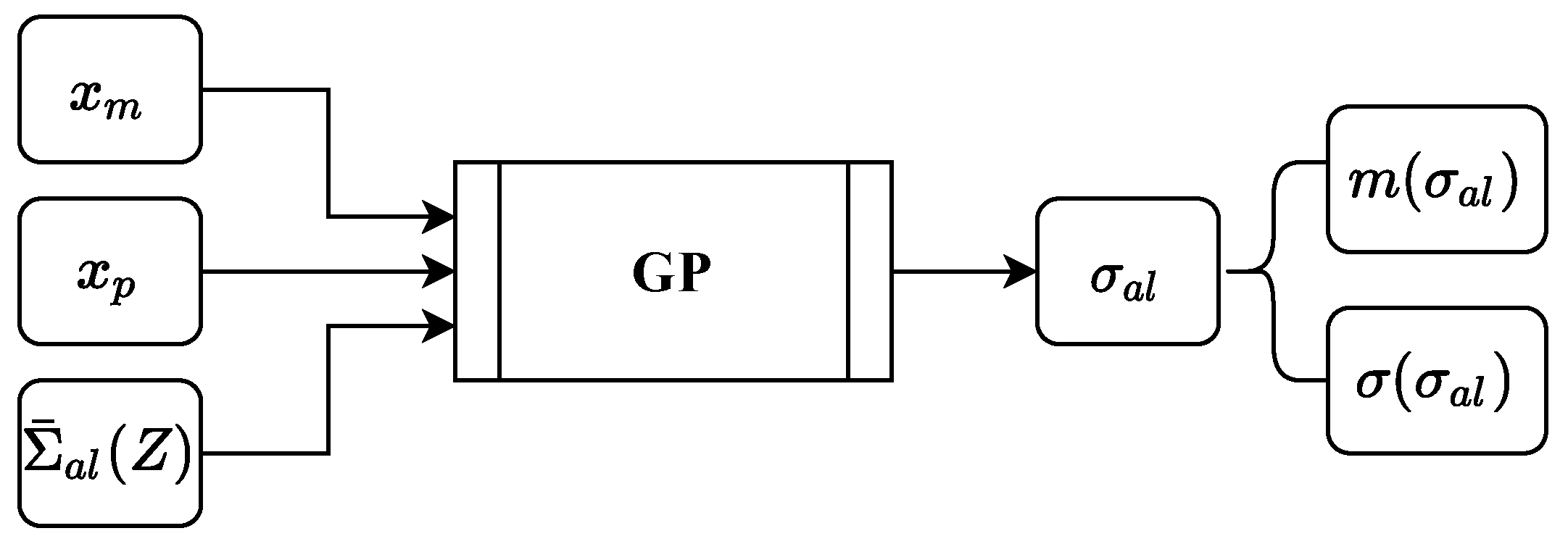
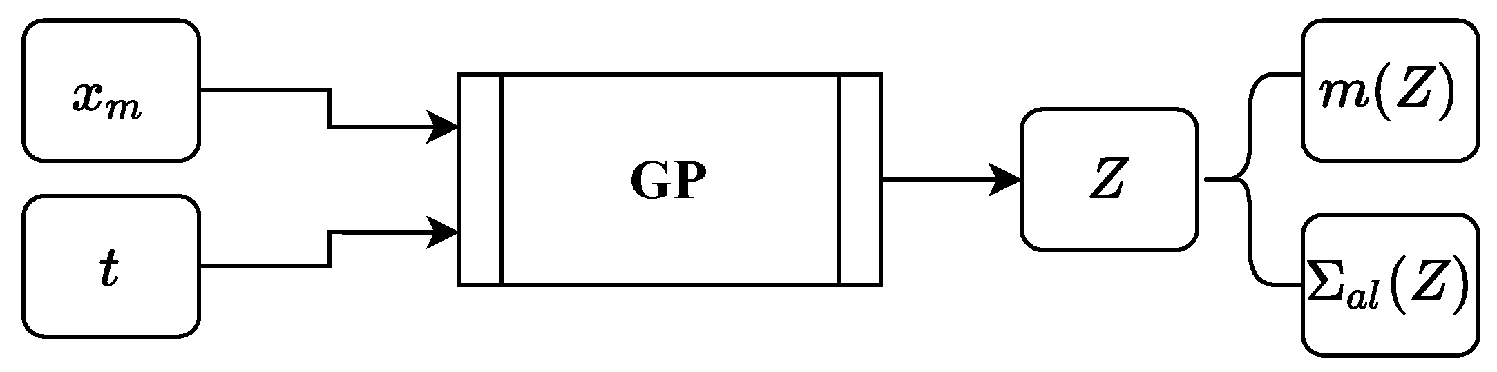
2.2. Aleatoric Uncertainty GP

A GP is used to predict a manufacturing process related aleatoric uncertainty ${\sigma }_{al}={\sigma }_{al}(x_m,x_p,{\overline{\mathsf{\Sigma }}}_{al}\left(\mathrm{Z}\right))$ of the manufactured part. Aleatoric uncertainty data are generated by uncertainty propagation analysis with FEM simulation. The inputs are the setting parameters from a real physical manufacturing process $x_m$, properties of the part to be manufactured $x_p$ and aleatoric manufacturing process uncertainty ${\overline{\mathsf{\Sigma }}}_{al}\left(\mathrm{Z}\right)$ obtained from, e.g., sensor data of the real physical manufacturing process, see Figure 2. Here, Z describes a characteristic of the manufacturing process, e.g., the velocity profile of a forming tool. The output ${\sigma }_{al}$ is predicted by a GP regression, such that ${\sigma }_{al}\sim \mathcal{GP}(m(x_m,x_p,{\overline{\mathsf{\Sigma }}}_{al}\left(\mathrm{Z}\right)),k((x_m,x_p,{\overline{\mathsf{\Sigma }}}_{al}\left(\mathrm{Z}\right)),$${(x_m,x_p,{\overline{\mathsf{\Sigma }}}_{al}\left(\mathrm{Z}\right))}^{\prime }\left)\right)$ with mean $m(x_m,x_p,{\overline{\mathsf{\Sigma }}}_{al}\left(\mathrm{Z}\right))$ and covariance function $k((x_m,x_p,{\overline{\mathsf{\Sigma }}}_{al}\left(\mathrm{Z}\right)),$${(x_m,x_p,{\overline{\mathsf{\Sigma }}}_{al}\left(\mathrm{Z}\right))}^{\prime })$.

Of course, a wide variety of manufacturing process characteristics can be implemented, e.g., rolling speeds, cutting forces, heating times etc. As a running example, we choose as a manufacturing process hot metal forming on a friction screwpress, where $x_m$ contains different input features which control the forging aggregate (clutch pressure between flywheels and rotation speed of the electric motor), $x_p$ describes the part to be forged by different dimensions and part temperature and Z is a resulting velocity profile of the forging tool over time for a given input $x_m$, where ${\overline{\mathsf{\Sigma }}}_{al}\left(\mathrm{Z}\right)$ represents aggregated aleatoric deviations in respect to forging velocity. ${\sigma }_{al}$ then describes the deviations of the final forged part, i.e., deviations from important final part geometries. All relevant details of our running example can be found in Section 4.

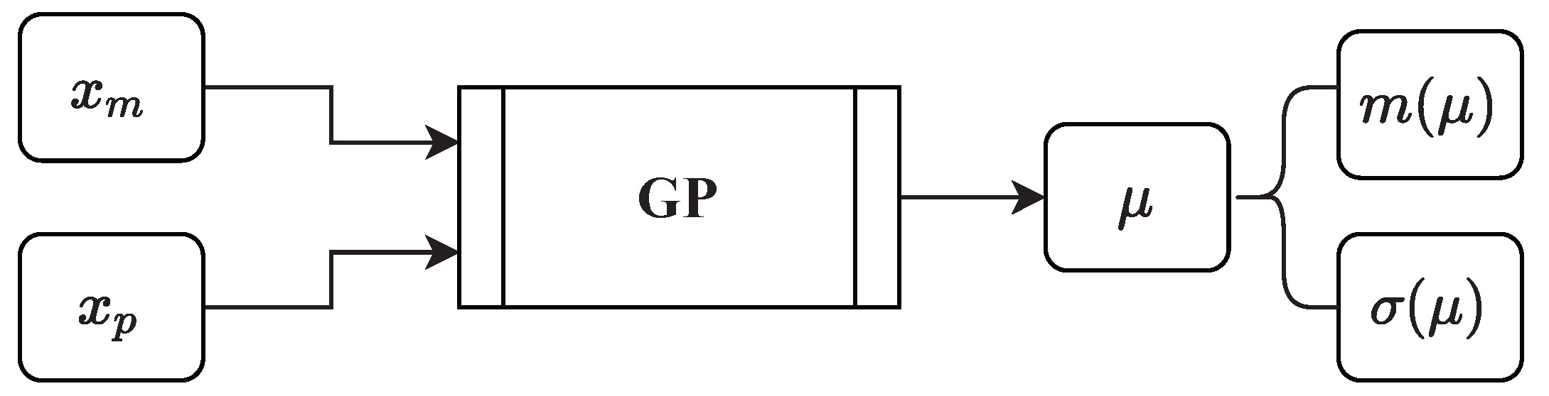
2.3. Mean Result GP

Besides the GP that predicts the aleatoric uncertainty of a manufactured part, a second GP is used to predict the mean result $\mu$ of the manufactured part. The inputs for the second GP are the setting parameters from the real physical manufacturing process $x_m$ and properties of the to be manufactured part $x_p$. The output $\mu$ is predicted by the GP regression, such that $\mu \sim \mathcal{GP}(m(x_m,x_p),k((x_m,x_p),{(x_m,x_p)}^{\prime }))$. In respect to our running example, $\mu$ describes the final forged part by important final part geometries.

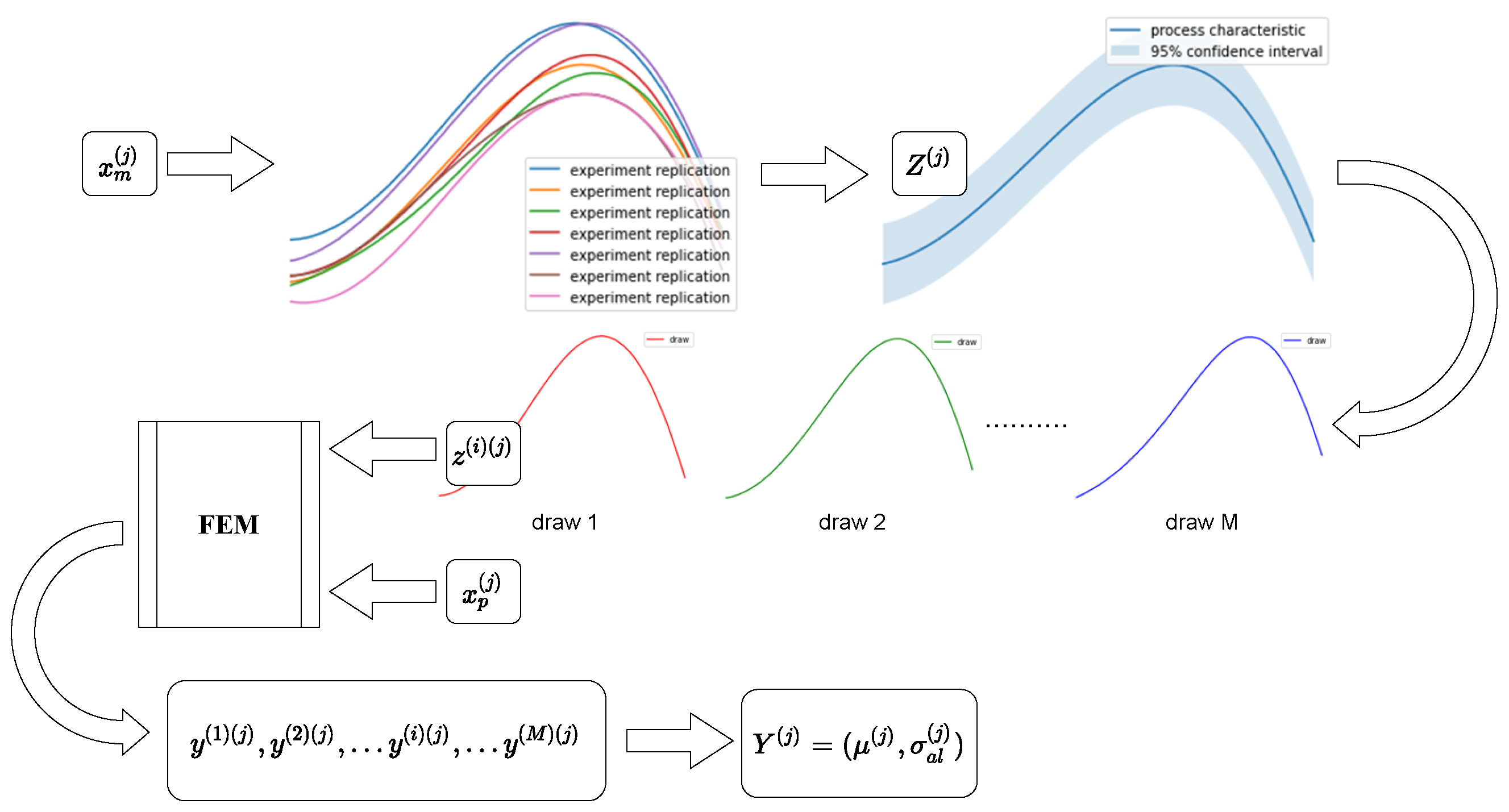
2.4. Uncertainty Propagation Analysis

In uncertainty propagation analysis, the effect of uncertainties related to an input on uncertainties of the corresponding output is investigated. In our case, ${\mathsf{\Sigma }}_{al}\left(\mathrm{Z}\right)$ refers to the aleatoric deviations of a manufacturing process characteristics (i.e., deviations in velocity profile data) due to different input settings. We refer to uncertainties with respect to a manufacturing process output obtained by uncertainty propagation analysis as aleatoric uncertainty ${\sigma }_{al}$.

We vary input values $x^{\left(j\right)}=(x_m^{\left(j\right)},x_p^{\left(j\right)})$ with $j\in \left\{1,\dots ,N\right\}$ where N is the number of different input setting scenarios. For each case of process-specific input parameters $x_m^{\left(j\right)}$, we obtain a process-specific characteristic ${\mathrm{Z}}^{\left(j\right)}$ that is a distribution with mean $m\left({\mathrm{Z}}^{\left(j\right)}\right)$ and standard deviation ${\mathsf{\Sigma }}_{al}\left({\mathrm{Z}}^{\left(j\right)}\right)$. Such distributions occur because, with identical input parameters, process characteristics in reality can show deviations when repeated. We simulate that behavior with a separate GP, thus, a random variable ${\mathrm{Z}}^{\left(j\right)}$ is assumed to be Normally distributed, such that ${\mathrm{Z}}^{\left(j\right)}=\mathcal{N}(m\left({\mathrm{Z}}^{\left(j\right)}\right),{\mathsf{\Sigma }}_{al}\left({\mathrm{Z}}^{\left(j\right)}\right))$. From the posterior, we randomly draw M predictions ${\mathrm{Z}}^{\left(i\right)\left(j\right)}$ with $i\in \left\{1,\dots ,M\right\}$ (i.e., different curves characterizing the manufacturing process) and with each ${\mathrm{Z}}^{\left(i\right)\left(j\right)}$ and $x_p^{\left(j\right)}$ we execute FEM simulations to obtain targets $y^{\left(i\right)\left(j\right)}$. We collect the individual targets $y^{\left(i\right)\left(j\right)}$, such that we obtain for each input setting j a distribution with mean ${\mu }^{\left(j\right)}$ and aleatoric standard deviation (i.e., aleatoric uncertainty) ${\sigma }_{al}^{\left(j\right)}$. With that, we are able to describe each target by its distribution.

Thus, we obtain a dataset $D=\left\{D^{\left(1\right)},\dots ,D^{\left(N\right)}\right\}$ where each datapoint $D^{\left(j\right)}=(X^{\left(j\right)},Y^{\left(j\right)})$ can then be separated into input $X^{\left(j\right)}=(x_m^{\left(j\right)},x_p^{\left(j\right)},{\overline{\mathsf{\Sigma }}}_{al}\left({\mathrm{Z}}^{\left(j\right)}\right))$ and output $Y^{\left(j\right)}=({\mu }^{\left(j\right)},{\sigma }_{al}^{\left(j\right)})$. Here ${\overline{\mathsf{\Sigma }}}_{al}\left({\mathrm{Z}}^{\left(j\right)}\right)$ is an aggregated manufacturing process uncertainty obtained from data. We model each output with a GP regression, thus the outputs are described again by a distribution with mean m and epistemic standard deviation $\sigma$ (i.e., epistemic uncertainty), such that ${\mu }^{\left(j\right)}=\mathcal{N}(m\left({\mu }^{\left(j\right)}\right),\sigma \left({\mu }^{\left(j\right)}\right))$ and ${\sigma }_{al}^{\left(j\right)}=\mathcal{N}(m\left({\sigma }_{al}^{\left(j\right)}\right),\sigma \left({\sigma }_{al}^{\left(j\right)}\right))$.

3. Active Learning and Solving Inverse Problems

For optimization, we evaluate our surrogate model in two different areas: (1) active learning and (2) solving multi-objective inverse problems. We refer to active learning as a method to find the most informative data points in the feature space for the best overall performance of the surrogate model, i.e., predicting the mean result of a manufacturing process $\mu$ and corresponding aleatoric uncertainty of the manufacturing result ${\sigma }_{al}$. When solving multi-objective inverse problems, we try to find inputs where the error between a given target vector and a prediction as well as the aleatoric uncertainty is minimal, leading to robust optimization results.

3.1. Active Learning

Active learning is already well researched in terms of optimal use of resources for parameter optimization of a model, i.e., generating training data, see [12,32,33,34]. The process of generating training data means obtaining labels $Y_{train}$ for an input $X_{train}$, such that a dataset $D_{train}=(X_{train},Y_{train})$ can be used to fit or optimize parameters of a model. Labels $Y_{train}$ are obtained by an oracle, where an oracle can be a domain expert, results of real physical experiments or like in our case results of expensive numerical FEM simulations. In the following, we present the idea behind the researched optimization approach and highlight the applicability of active learning with our proposed surrogate model.

In active learning, a number of $n_{AL}$ datapoints connected to maximum epistemic uncertainty ${\sigma }_{ep}$ are queried from a pool of candidates $X_{pool}$ to build a training dataset $D_{train}=(X_{train},Y_{train})$ that is used for training a surrogate model. Thus, we select ideal training data, i.e., we use a minimum amount of training data such that the overall epistemic uncertainty in respect to making prediction on $X_{pool}$ is minimized. We define in (11) the active learning query strategy with loss function ${\mathcal{L}}_{AL}={\mathcal{L}}_{AL}\left({\sigma }_{ep}\right)={\sigma }_{ep}\left(x\right)$ to select a new query datapoint $d_q^{AL}=(x_q^{AL},y_q^{AL})$ with input $x_q^{AL}$ and output $y_q^{AL}$.

$$d_q^{AL}=\underset{xin{X}_{pool}}{argmax}{\sigma }_{ep}\left(x\right)$$

(11)

A query datapoint $d_q^{AL}$ is then moved to the training dataset $D_{train}$, the surrogate model is fitted and the iterative generation of training data starts again. In respect to our proposed surrogate model, we are able to utilize directly the epistemic uncertainty predictions of the two GPs, i.e., $\sigma \left(\mu \right)$ and $\sigma \left({\sigma }_{al}\right)$. Thus, we define ${\sigma }_{ep}\left(x\right)=\sigma \left(\mu \left(x\right)\right)+\sigma \left({\sigma }_{al}\left(x\right)\right)$ and select training data by utilizing (11).

3.2. Inverse Problem

In real physical manufacturing processes, it is commonly required that the result of the manufacturing process lies within a given tolerance range. Therefore, the parameters that control the manufacturing process and the properties of the part must be carefully selected. Moreover, the process of finding inputs to obtain a given target can be formulated as an inverse problem, i.e., finding causal factors for a required effect. In our work, we define that a basic solution of an inverse problem is to find an input $x_{inv}$, minimizing a distance $d=d(y_{inv},y_{target})$ between prediction $y_{inv}$ and target vector $y_{target}$. However, such solutions neglect the existence of process variations, i.e., aleatoric uncertainty. With no consideration of aleatoric uncertainty, the found ideal inputs can lead to quite good results regarding mean values but very high deviations, such that no robustness assertions can be made.

Therefore, we present a novel multi-objective optimization approach in (12) based on BO with a modified UCB acquisition function, where we make a clear separation of uncertainties, such that a loss function ${\mathcal{L}}_{inv}$, dependent of a distance function d, respective aleatoric ${\sigma }_{al}$ and epistemic ${\sigma }_{ep}$ uncertainties is minimized.

$$x_{inv}=\underset{X_{pool}}{argmin}{\mathcal{L}}_{inv}(d,{\sigma }_{al},{\sigma }_{ep})$$

(12)

As a distance function d, we select the absolute error between mean target ${\mu }_{target}$ and mean manufacturing process result $m\left(\mu \right)$ as the metric. However, our approach is not limited to a specific distance metric, so any can be used.

$$d=d({\mu }_{target},m\left(\mu \right))=|{\mu }_{target}-m\left(\mu \right)|$$

(13)

Utilizing $m\left({\sigma }_{al}\right)$, $\sigma \left({\sigma }_{al}\right)$, $m\left(\mu \right)$ and $\sigma \left(\mu \right)$ from our proposed surrogate model, we define epistemic uncertainty ${\sigma }_{ep}={\sigma }_{ep}(\sigma \left({\sigma }_{al}\right),\sigma \left(\mu \right))=\sigma \left({\sigma }_{al}\right)+\sigma \left(\mu \right)$ and construct a loss function ${\mathcal{L}}_{inv}$ with tuning parameters $\alpha$ and $\beta$, where $\alpha$ controls the influence of the aleatoric uncertainty and $\beta$ controls exploration vs. exploitation, i.e., the influence of the epistemic uncertainty.

$$\begin{array}{c}\hfill {\mathcal{L}}_{inv}(d({\mu }_{target},m\left(\mu \right)),m\left({\sigma }_{al}\right),{\sigma }_{ep}(\sigma \left({\sigma }_{al}\right),\sigma \left(\mu \right)))=\\ \hfill d({\mu }_{target},m\left(\mu \right))+\alpha ·m\left({\sigma }_{al}\right)-\beta ·{\sigma }_{ep}(\sigma \left({\sigma }_{al}\right),\sigma \left(\mu \right)))\end{array}$$

(14)

Thus, with our approach, we find inputs that provide robust outputs close to a given target while keeping aleatoric uncertainty low. As a result, we obtain robust optimization outcomes when solving multi-objective inverse problems with our approach. In the work of Dai Nguyen et al. [25] we found a similar handling of uncertainty in the observation of the acquisition function, however, the authors only focus on maximizing black box functions, while we present an extension that solves multi-objective inverse problems.

4. Case Study on Forging Superalloys

We evaluate the proposed surrogate model and novel optimization method with a classic use case from the field of hot metal forming, preforming an Inconel 625 superalloy billet on an artificially designed forging press. First, we design the forging press characteristics with a parameterized curve and a GP and second, we design the forming process itself in a FEM simulation environment where we provide all the relevant information so that it is possible for researchers to link directly to our work.

4.1. Forging Aggregate Characteristic

We calculate the mean forming velocity values of an artificially designed forging process on the example of a forging screwpress by a self-designed parameterized curve in (15) that models the die velocity $v_{die}$ in mm/s as a function of the process timestep t in $seconds$, clutch pressure $x_1$ in $bar$ and rotation speed of the electric motor $x_2$ in rpm, such that $v_{die}=v_{die}(x_1,x_2,t)$. Where, $x_1$ and $x_2$ are two process-specific setting parameters, i.e. $x_m=(x_1,x_2)$.

$$v_{die}(x_1,x_2,t)={\kappa }_1·x_1·x_2·t^2-{\kappa }_2·x_1·x_2·t^3$$

(15)

where ${\kappa }_1=\frac{5}{3}$ mm${}^2$/kg and ${\kappa }_2=\frac{5}{3}$ mm${}^2$/kgs are constants. We utilize a designed forging press specific GP with data generated by using (15) to model the mean and input dependent deviations in respect to the manufacturing process characteristic Z (i.e., Z represents the velocity profile of the forging die $v_{die}$). Z is defined by a distribution with mean $m\left(\mathrm{Z}\right)$ and aleatoric standard deviation ${\mathsf{\Sigma }}_{al}\left(\mathrm{Z}\right)$. With respect to our use case, the forging press specific GP with output ${\mathrm{Z}}^{\left(j\right)}$ is at the very beginning of the uncertainty propagation analysis, see Figure 4. The inputs for the forging press GP are $x_m=(x_1,x_2)$ and time increments $t=\left\{0,\dots ,T\right\}$, where T represents the duration of the manufacturing process. The output of the forging press GP is Z, such that $\mathrm{Z}\sim \mathcal{GP}(m(x_m,t),k((x_m,t),{(x_m,t)}^{\prime }))$ with mean $m(x_m,t)$ and covariance function $k((x_m,t),{(x_m,t)}^{\prime })$. Thus, we obtain for each time increment a distribution describing the velocity at time t. The principle GP design for the forging press can be seen in Figure 5. As covariance function, k we found out that an RBF kernel is appropriate.

We utilize (15) and different input parameter combinations to generate training data for the forging press GP, see

Table 1. Input parameter combinations to generate training data for the forging press GP.

Training Data for Forging Press GP
$x_1$	12	12	12	16	16	16	20	20	20
$x_2$	50	60	70	50	60	70	50	60	70

. In terms of time step size t, we assume that each forging stroke lasts one second, and we model each stroke with a resolution of 100 time steps.

To obtain different deviations connected to different $x_1$ and $x_2$ combinations, we use the underlying inference properties of GP regression and vary inter- and extrapolation tasks in respect to the input values for forging process representation, see

Table 2. Input parameter combinations to model forging press characteristics.

Evaluation Data for Forging Press Characteristics
$x_1$	10	10	10	10	14	14	14	14	18	18	18	18	22	22	22	22
$x_2$	45	55	65	75	45	55	65	75	45	55	65	75	45	55	65	75

.

We define interpolation such that a value is within the training range (i.e., $x_1$ equals 14 or 18 and $x_2$ equals 55 or 65) and extrapolation such that a value is out of the training range (i.e., $x_1$ equals 10 or 22 and $x_2$ equals 45 or 75).

Exemplary forging press characteristics can be seen in Figure 6, where Figure 6a shows low deviation because $x_1$ and $x_2$ are both lie within the range of training data, Figure 6b,c show moderate deviation because one of the process parameters is within and the other is outside the range of the training data and Figure 6d shows the highest deviation because both of the process-parameters lie outside the range of training data. Thus, our forging press GP represents a forging aggregate characteristics with uncertainties dependent on the inputs. In our approach, we intentionally generate deviations depending on input parameters and assume that uncertainty is aleatoric to approximate reality, i.e., we abuse epistemic uncertainty and assume that it is aleatoric. When working with sensor data coming from a real manufacturing process, it is obvious that deviations, i.e., aleatoric process uncertainties ${\mathsf{\Sigma }}_{al}$, can be directly measured from data.

4.2. FEM Simulation

The considered use case, preforming an Inconel 625 superalloy billet on a forging press machine, is observed by utilizing a corresponding FEM simulation. Manufacturing process related FEM inputs ${\mathrm{Z}}^{\left(j\right)}$, i.e., different velocity profiles of the upper die over time, are modeled by the forging press GP. Inputs for the forging press GP are $x_1$, $x_2$ and t, such that ${\mathrm{Z}}^{\left(j\right)\left(t\right)}={\mathrm{Z}}^{\left(j\right)\left(t\right)}(x_1^{\left(j\right)},x_2^{\left(j\right)},t)$. 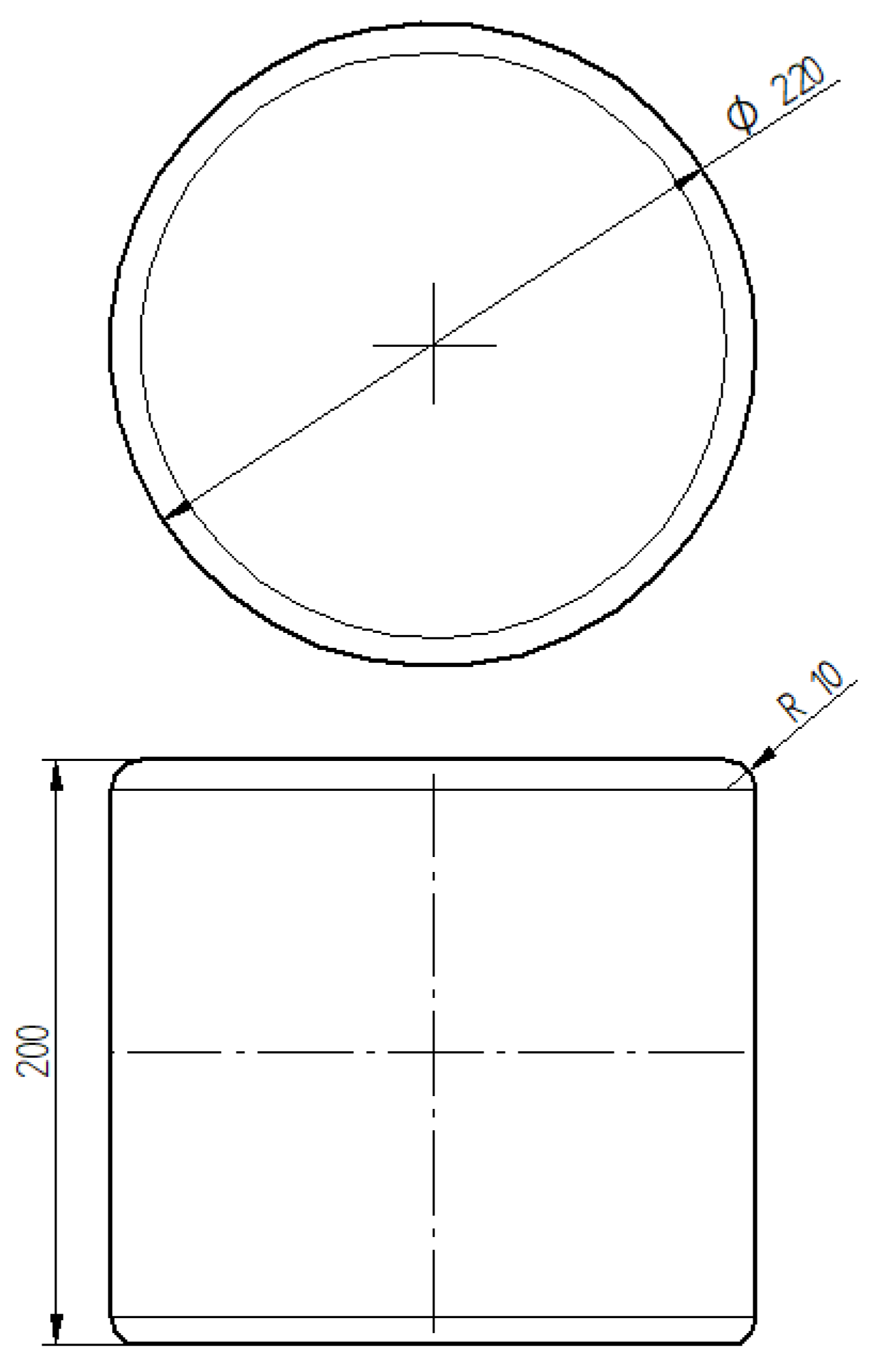All 16 possible combinations for manufacturing process related FEM inputs are shown in Table 2. Billet related inputs $x_p^{\left(j\right)}$ that are shared with our proposed surrogate model and FEM simulation are diameter, height and temperature, such that $x_p^{\left(j\right)}=(d^{\left(j\right)},h^{\left(j\right)},{\theta }^{\left(j\right)})$. One possible billet configuration is shown in Figure 7 and possible billet parameters for different configurations are shown in

Table 3. Key parameters for billet configurations $x_p^{\left(j\right)}$, values in mm.

Configuration Data
Diameter d	220	240	260
Height h	200	210	220
Temperature $\theta$	900	1000	1100

. We define the radius of the rounded edges to be constant 10 mm across all configurations.

We observe in total 27 different billets. Connecting manufacturing process related combinations with different billets, we obtain 432 combinations, i.e., $j\in \left\{1,\dots ,432\right\}$. For evaluation of the uncertainty propagation, we randomly draw ${\mathrm{Z}}^{\left(i\right)\left(j\right)}$ with $i\in \left\{1,\dots ,20\right\}$ from each distribution ${\mathrm{Z}}^{\left(j\right)}$, i.e., 20 FEM simulations are performed for each input setting. Thus, a total of 8640 FEM simulation results are generated for our experiments. Selected FEM output variables for our surrogate model are the final diameter and height of the preformed billet, such that $y^{\left(i\right)\left(j\right)}=(d_{final}^{\left(i\right)\left(j\right)},h_{final}^{\left(i\right)\left(j\right)})$ and $Y^{\left(j\right)}=(\mu \left(d_{final}^{\left(j\right)}\right),\mu \left(h_{final}^{\left(j\right)}\right),{\sigma }_{al}\left(d_{final}^{\left(j\right)}\right),{\sigma }_{al}\left(h_{final}^{\left(j\right)}\right))$. In respect to the final diameter $d_{final}$, we calculate the empiric mean by $\mu \left(d_{final}^{\left(j\right)}\right)=\frac{1}{20}{\sum }_{i=1}^{20}{d}_{final}^{\left(i\right)\left(j\right)}$ and aleatoric standard deviation by ${\sigma }_{al}{\left(d_{final}^{\left(j\right)}\right)}^2=\frac{1}{20}{\sum }_{i=1}^{20}{(d_{final}^{\left(i\right)\left(j\right)}-\mu \left(d_{final}^{\left(j\right)}\right))}^2$. The calculations are analogous with respect to $h_{final}$. Thus, we obtain a dataset with 432 instances described by six input features and four output features. For our running example, input features are clutch pressure, rotation speed, initial billet diameter, initial billet height, initial billet temperature and aggregated manufacturing process uncertainties obtained from data, i.e., the aggregated output of the forging press GP ${\overline{\mathsf{\Sigma }}}_{al}\left({\mathrm{Z}}^{\left(j\right)}\right)={\sum }_{t=1}^T{\mathsf{\Sigma }}_{al}{\left(\mathrm{Z}\right)}^{\left(j\right)\left(t\right)}$. Output features are the mean of the final billet diameter, the mean of the final billet height, the aleatoric uncertainty of the final billet diameter and the aleatoric uncertainty of the final billet height.

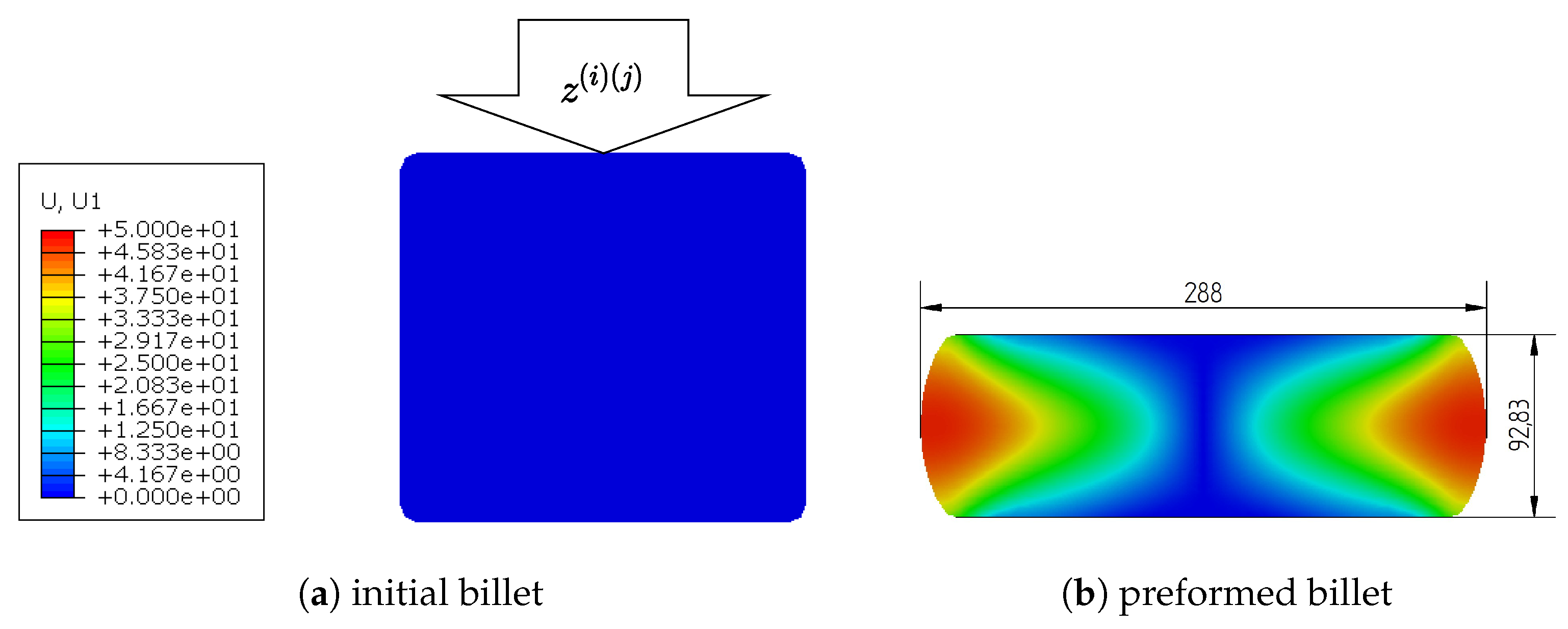
The problem is defined as a 2D axisymmetric simulation task to utilize symmetries and make efficient use of computational resources. We utilize isotropic elasto-plastic Inconel 625 material behavior from literature. The Young’s modulus is temperature-dependent and the yield stress depends on plastic strain, strain-rate and temperature. We set contact properties to tangential behavior with isotropic directionality and a friction coefficient of 0.3 between the billet and upper and lower forging tool, which means that we assume lubricated hot forging conditions. The lower tool is encastred and the upper tool’s boundary conditions are set so that the vertical movement ${\mathrm{Z}}^{\left(i\right)\left(j\right)}$ is drawn from distribution ${\mathrm{Z}}^{\left(j\right)}$ and there is no horizontal movement. An exemplary simulation definition can be seen in Figure 8, where (a) shows the initial state of the billet loaded with a randomly drawn screwpress velocity profile ${\mathrm{Z}}^{\left(i\right)\left(j\right)}$ and (b) the end result of the simulation with selected FEM output variables $y^{\left(i\right)\left(j\right)}$, i.e., the final diameter of 288 mm and the final height of 92.83 mm.

All billets are meshed with an approximate global element size of 7 mm, using 4-node bilinear axisymmetric quadrilateral elements with reduced integration and hourglass control. We obtain our FEM simulation results in the context of general static simulations. Details of the simulation steps are shown in

Table 4. Abaqus FEM simulation control parameters for our use case.

Abaqus FEM Simulation Settings
Simulation type	Static, General
Time period	1
Nlgeom	On
Max number of increments	1000
Initial increment size	0.001
Min increment size	1 × 10−5
Max increment size	1
Equation solver method	Direct
Solution technique	Full Newton

. Simulation control parameters that are not listed are left at default values.

5. Results

5.1. GPs

Before utilizing optimization methods, we evaluate each individual GP, see

Table 5. Evaluation of individual GPs by average R2-Scores over 10 folds.

Individual GP Evaluations
	Screwpress	Aleatoric Uncertainty		Mean Result
	$m\left(\mathrm{Z}\right)$	$m\left({\sigma }_{al,d_{final}}\right)$	$m\left({\sigma }_{al,h_{final}}\right)$	$m\left({\mu }_{d_{final}}\right)$	$m\left({\mu }_{h_{final}}\right)$
R2-Score	0.9923	0.8146	0.8455	0.9586	0.9555

. The screwpress GP is trained with data that is generated by using inputs from Table 1 with (15) and tested on data generated by using inputs from Table 2 with (15). As covariance function, k we found out that an RBF kernel is appropriate for this GP. The GPs of our proposed surrogate model are both designed with a Matérn kernel with $\nu =2.5$ and are independently evaluated by 10-fold cross-validation with inputs from Table 2 and ${\mathrm{Z}}^{\left(j\right)}$ obtained from the screwpress GP. Outputs are obtained from FEM simulations, see Section 4.2. In each cross-validation step, we split the respective data randomly such that 10 percent are in the test dataset and the remaining 90 percent are used for model training.

In addition, we calculate mean Pearson kurtosis

$$kur{t}_{Pearson}=\frac{1}{N}\sum _{j=1}^N\frac{1}{M}\sum _{i=1}^M{\left(\frac{y^{\left(i\right)\left(j\right)}-{\mu }^{\left(j\right)}}{{\sigma }_{al}^{\left(j\right)}}\right)}^4$$

(16)

and mean Fisher-Pearson coefficient of skewness

$$ske{w}_{Fisher-Pearson}=\frac{1}{N}\sum _{j=1}^N\frac{1}{M}\sum _{i=1}^M{\left(\frac{y^{\left(i\right)\left(j\right)}-{\mu }^{\left(j\right)}}{{\sigma }_{al}^{\left(j\right)}}\right)}^3$$

(17)

to describe the distribution shapes obtained from uncertainty propagation analysis, see

Table 6. Mean values of Pearson kurtosis and Fisher-Pearson coefficient of skewness calculated from uncertainty propagation analysis results.

Distribution Properties
	$d_{final}$	$h_{final}$
$kur{t}_{Pearson}$	3.003	2.685
$ske{w}_{Fisher-Pearson}$	0.449	0.015

.

GP models were implemented with the GPflow library version 2.2.1 and Python 3.8.10. Inferences were run on a machine with 16 GB RAM, 8 CPUs and Intel(R) i7-8565 2.0 GHz processor. We utilized a L-BFGS-B algorithm to train the models. Training our surrogate model on all available data took an average of 1.36 s based on 10 measurements. For one prediction our model needs on average 0.046 s. A FEM simulation lasted on average 149.78 s.

5.2. Active Learning

We evaluate our proposed surrogate model by using active learning and compare it with an approach based on random training data selection. Evaluation is based on 10-fold cross-validation. In each cross-validation step, models are initially trained on two randomly selected datapoints out of the pool dataset containing 432 instances. Evaluation metrics are R2-Score and mean-squared-error (MSE) and are computed on a 20 percent hold-out test set that is randomly generated in each cross-validation step. Results for the mean of reduced-order predictions and corresponding aleatoric uncertainties regarding final diameter and height are shown respectively in Figure 9 and Figure 10, where solid lines depict the mean R2-Score values and shaded areas are obtained by adding and subtracting one standard deviation. Mean values and standard deviations are calculated from the 10 cross-validation results.

5.3. Solving Inverse Problem

We evaluate our proposed multi-objective optimization strategy by solving inverse problems, i.e., we try to find input settings that lead to an output that is as near as possible to an initially defined target vector. In addition to minimize distances between a target vector $y_{target}$ and random mean vector $m\left({\mu }^{\left(j\right)}\right)$, we try to achieve results that also keep mean aleatoric uncertainty $m\left({\sigma }_{al}^{\left(j\right)}\right)$ low. We utilize a 10-fold cross-validation, where in each cross-validation step the target vector is randomly drawn from the pool dataset and the best found prediction after drawing 50 datapoints out of the pool dataset is used for evaluation. This means that for each method, a dataset of 50 datapoints is generated, and each best prediction is found by evaluating the respective acquisition function on the corresponding generated dataset. We compare our approach with two other baselines, namely:

(1)

Combined (This baseline can be considered as an approximation to the use of heteroskedastic GP in UCB BO.): no distinction of uncertainties in UCB based BO, i.e., simply adding aleatoric and epistemic uncertainty with loss:

$$\begin{array}{c}\hfill {\mathcal{L}}_{combined}(d({\mu }_{target},m\left(\mu \right)),m\left({\sigma }_{al}\right),{\sigma }_{ep}(\sigma \left({\sigma }_{al}\right),\sigma \left(\mu \right)))=\\ \hfill d({\mu }_{target},m\left(\mu \right))-[\alpha ·m\left({\sigma }_{al}\right)+\beta ·{\sigma }_{ep}(\sigma \left({\sigma }_{al}\right),\sigma \left(\mu \right)))]\end{array}$$

(18)

(2)

Epistemic: neglecting aleatoric uncertainty in UCB based BO with loss:

$$\begin{array}{c}\hfill {\mathcal{L}}_{epistemic}(d({\mu }_{target},m\left(\mu \right)),m\left({\sigma }_{al}\right),{\sigma }_{ep}(\sigma \left({\sigma }_{al}\right),\sigma \left(\mu \right)))=\\ \hfill d({\mu }_{target},m\left(\mu \right))-\beta ·{\sigma }_{ep}(\sigma \left({\sigma }_{al}\right),\sigma \left(\mu \right))).\end{array}$$

(19)

Figure 11 shows representative plots of optimization results for one random target vector (i.e., one cross-validation step) over 50 draws of $x_{inv}$, where solid lines depict squared errors and dotted lines show mean aleatoric uncertainty $m\left({\sigma }_{al}\right)$. Figure 12 and Figure 13 show different distributions of optimization results obtained by 10-fold cross-validation in respect to squared errors and mean aleatoric uncertainty $m\left({\sigma }_{al}\right)$. Distributions are visualized by kernel density estimation.

6. Discussion

Evaluation of the individual GPs with 10-fold cross-validation shows promising R2-Scores (lowest: 0.8146, mean: 0.89355, highest: 0.9586), i.e., hyperparameters appear to be appropriate for further evaluations. Observation of generated manufacturing process uncertainties, i.e., ${\overline{\mathsf{\Sigma }}}_{al}\left({\mathrm{Z}}^{\left(j\right)}\right)$ shows a diverse data landscape, thus, we assume that further uncertainty propagation analysis is meaningful.

We observe the distributions obtained from uncertainty propagation analysis by calculating Pearson kurtosis and Fisher-Pearson coefficient of skewness (A Pearson kurtosis of $3.0$ and Fisher-Pearson coefficient of skewness of $0.0$ describe a normal distribution). Regarding kurtosis, results shows that distributions are near to Normal distributions, where the distribution of $h_{final}$ is slightly platykurtic ($kur{t}_{Pearson}\left(h_{final}\right)=2.685<3.0$), i.e., it is less peaked than a Normal distribution and the distribution of $d_{final}$ is little leptokurtic ($kur{t}_{Pearson}\left(d_{final}\right)=3.003>3.0$), i.e., the distribution is more peaked compared to a Normal distribution. In terms of skewness, the distribution of $d_{final}$ is more skewed compared to $h_{final}$, however, both values are less than 0.5 so that approximate symmetry can be assumed.

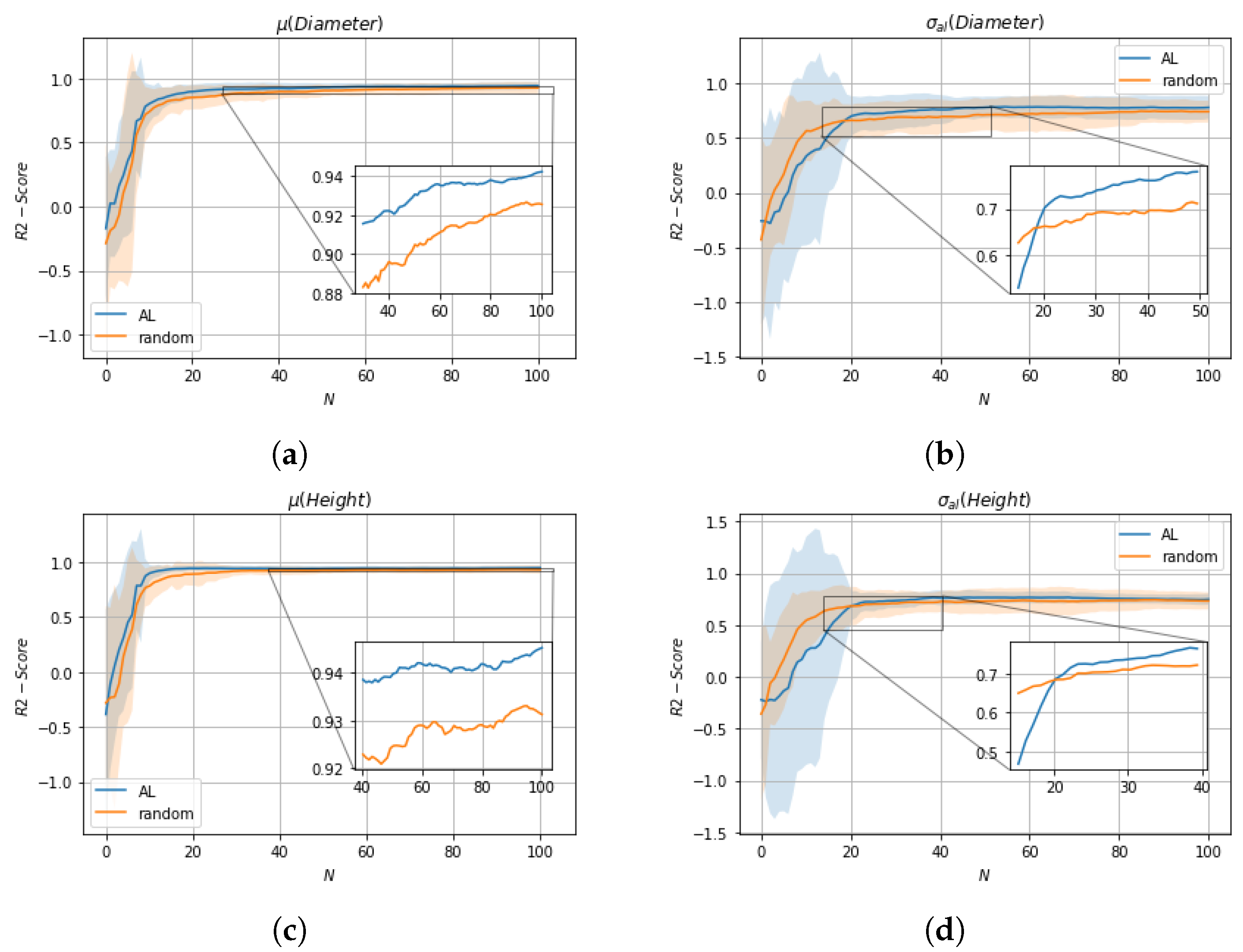
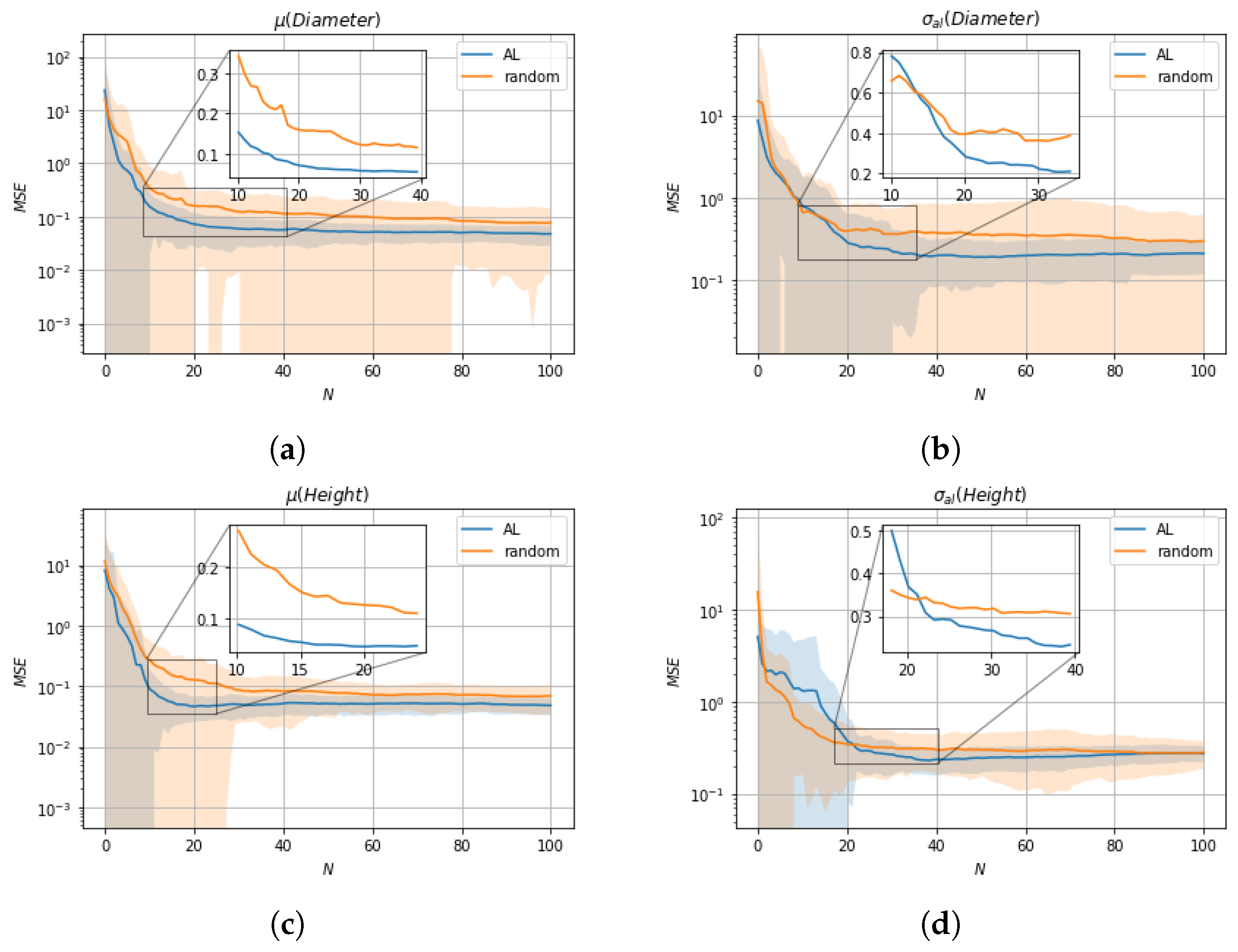
We evaluate the impact of data selection for model training using two metrics, R2-Score and MSE, with a 10-fold cross-validation comparing active learning with random sample selection. With respect to mean values $\mu$, active learning shows overall an improvement compared to random sample selection. In terms of aleatoric uncertainties ${\sigma }_{al}$, random sample selection is superior to active learning up to the selection of about 20 samples, but after that active learning shows superior performance compared to random sample selection. The initially worse performance of active learning with respect to ${\sigma }_{al}$ is due to a trade-off in the active learning cost function between $\sigma \left(\mu \right)$ and $\sigma \left({\sigma }_{al}\right)$ with the influence of $\sigma \left(\mu \right)$ dominating. A possible solution for this would be the introduction of appropriate tuning parameters that regulate the influence of the respective epistemic uncertainties $\sigma \left(\mu \right)$ and $\sigma \left({\sigma }_{al}\right)$. Moreover, it should be noted that random sample selection shows only better performance at a stage where the tuning of parameters is far from complete, so the better performance is not applicable in practice.

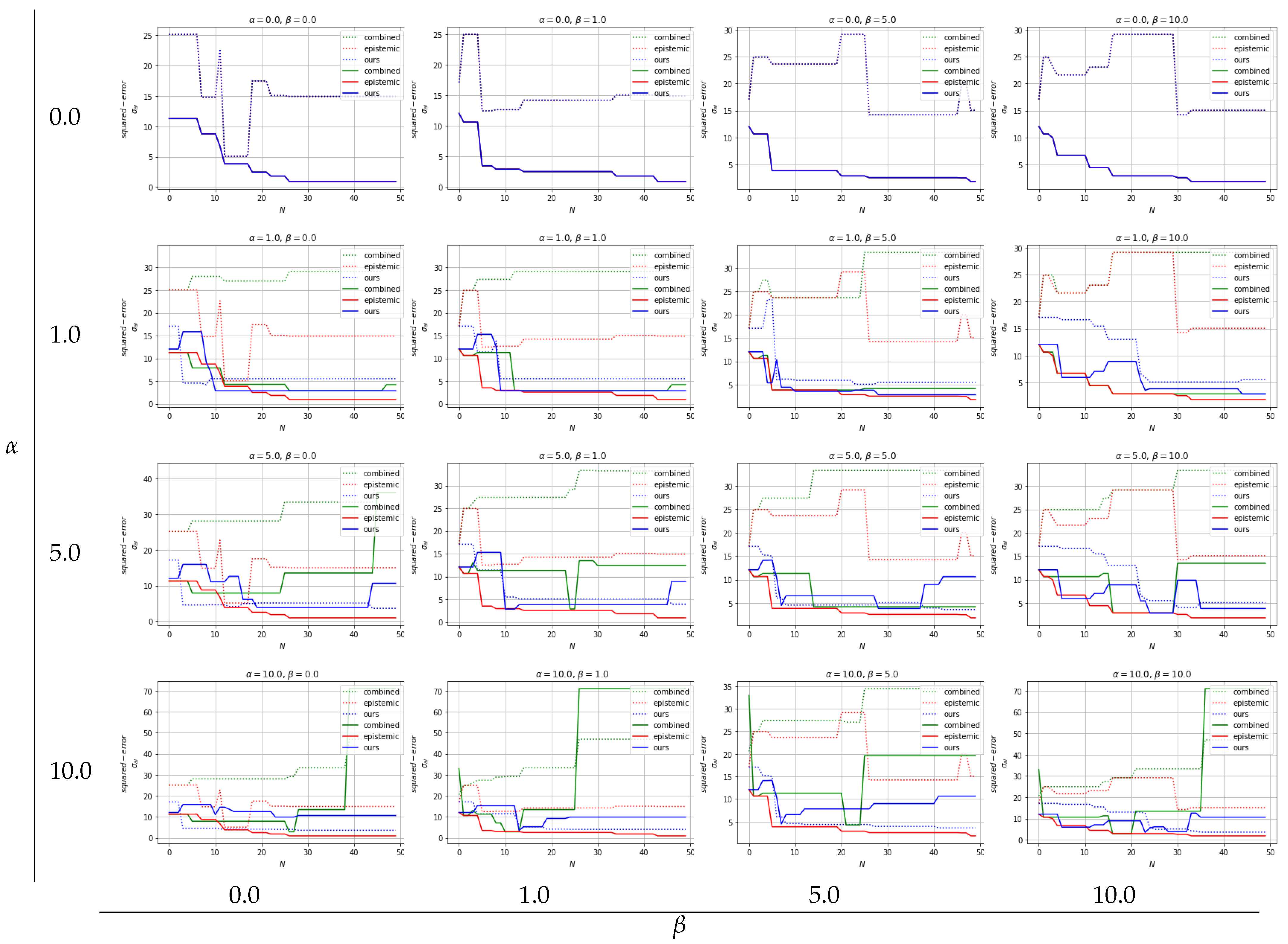
With regard to solving inverse problems, we compare our novel robust UCB based BO multi-objective optimization algorithm with two baselines: (1) combined: no distinction of uncertainties in UCB based BO and (2) epistemic: neglecting aleatoric uncertainty in UCB based BO. We show that over different values of tuning parameters $\alpha$ and $\beta$ there are clear tendencies of the different approaches. By disabling the influence of aleatoric uncertainty ($\alpha =0$), all three approaches show the same results as expected: low squared errors and neglected aleatoric uncertainty. For all approaches, slight differences can be seen over different $\beta$ values while $\alpha =0$, regulating the exploration vs. exploitation trade-off.

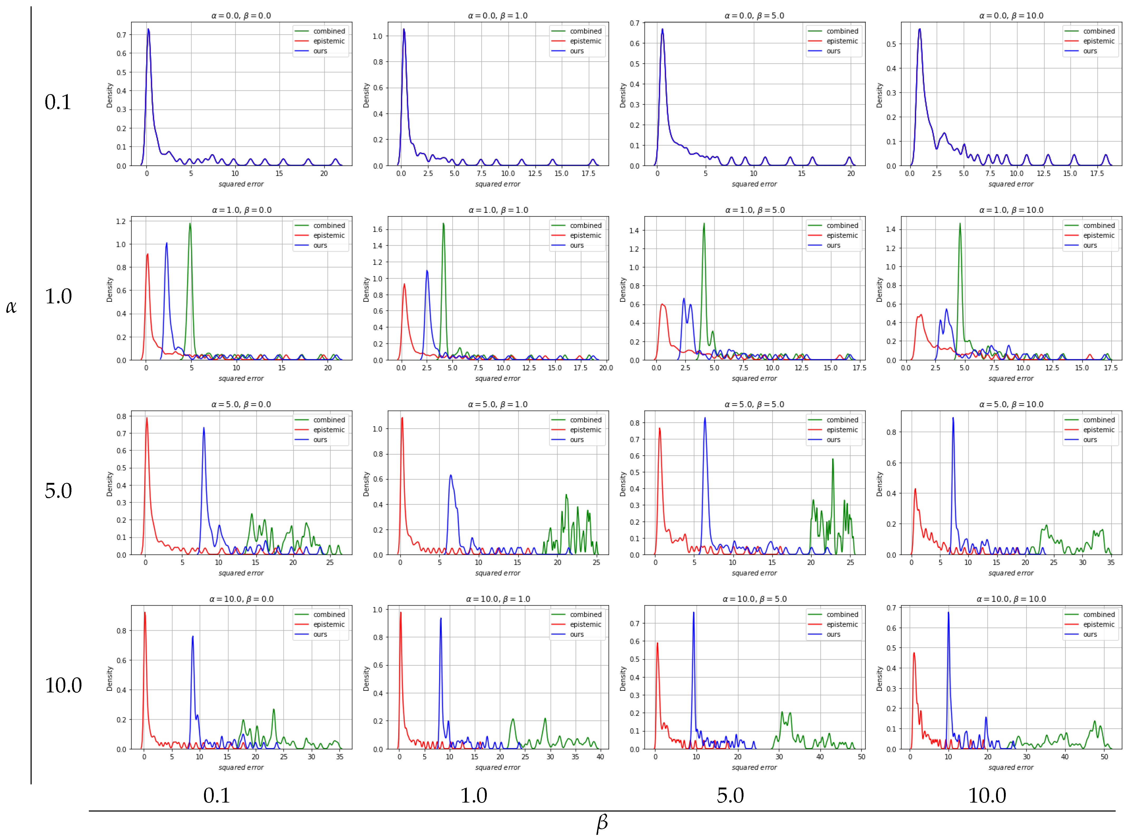
Due to the fundamentals of the epistemic approach, there are no differences in the optimization result when $\alpha$ values are changed for constant $\beta$ values, see Figure 11. Differences in kernel density estimate plots over varying $\alpha$ values are from random target vector selection. 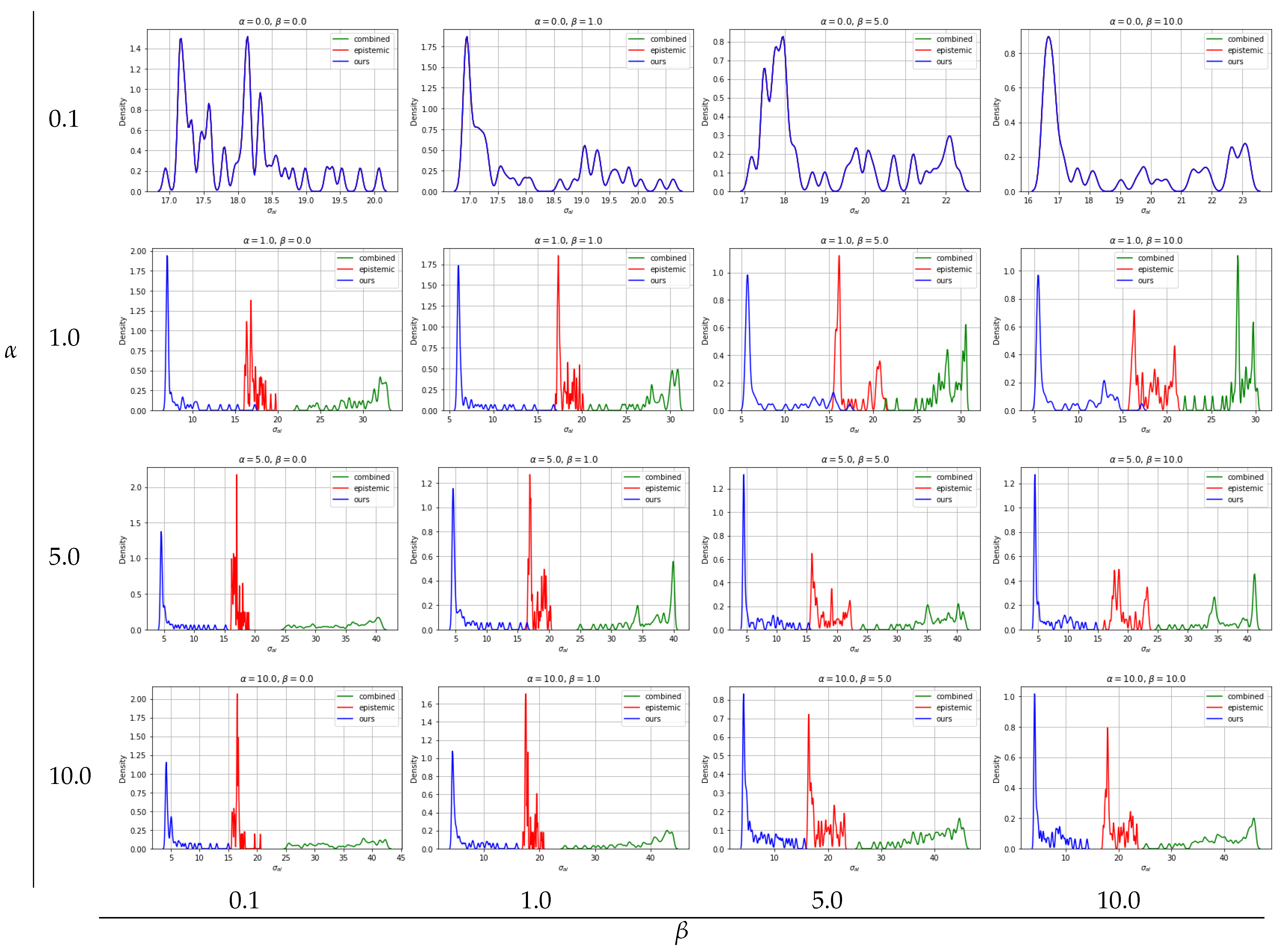Overall, the epistemic approach yields the best optimization results in terms of squared errors, see Figure 11 and Figure 12, however, as expected, aleatoric uncertainty is ignored and thus high, see Figure 13. The combined approach, where aleatoric and epistemic uncertainties are simply added and handled as quasi-epistemic, shows the overall worst results. At low $\alpha$ values, the squared errors are acceptable, but the aleatoric uncertainty is high due to inappropriate handling of information, see Figure 11, Figure 12 and Figure 13. To arrive at our approach, once aleatoric uncertainty is considered, i.e., $\alpha >0.0$ results for the inverse problem show low squared errors and low aleatoric uncertainty which we recognize as robust results. Moreover, by increasing $\alpha$ one can see that our approach leads to results where lowering aleatoric uncertainty ${\sigma }_{al}$ is more preferred than lowering squared errors, see Figure 11$\alpha =1.0$ and $\alpha =10.0$. Kernel density estimate plots generated from 10-fold cross-validation results confirm those findings, where clear tendencies of optimization results in respect to tuning parameters $\alpha$ and $\beta$ can be seen. While an approach considering only epistemic uncertainties delivers overall best results in respect to squared errors, aleatoric uncertainties are out of scope, thus, optimization results lead to less robust outcomes. An approach considering aleatoric and epistemic uncertainties combined by summing them up shows overall worst results and can not compete with the remaining. Our approach, where aleatoric and epistemic uncertainties are considered to deliver different information, depicts that overall good results are achieved with respect to squared errors while keeping aleatoric uncertainty low, thus robust solutions for solving multi-objective inverse problems are provided.

Moreover, our model is directly applicable in an industrial framework where the forging press characteristics are represented by measured sensor data of the aggregate (e.g., velocity over time, forging force over time, forging force over the forming path, etc.), which can be used in an appropriately designed FEM simulation for uncertainty propagation analysis and, moreover, for surrogate model training.

7. Conclusions

In this work, we present a GP based reduced-order surrogate model approach with a novel multi-objective target vector optimization strategy to obtain more robust optimization results by concerning aleatoric and epistemic uncertainties. Evaluation on a classic hot metal forming use case, preforming an Inconel 625 forging billet on a self-designed forging press, depicts the advantages of our approach compared to baselines. Our major findings include that our surrogate model produces fast results (over 3000 times faster) compared to FEM simulation, with a calculated loss of accuracy and information. Moreover, active learning can be used directly with our model to make optimal use of computational resources, and solving inverse problems leads to robust optimization results, i.e., finding results close to a defined objective while keeping aleatoric uncertainty low. With our work, we pave one promising way for faster and more realistic simulation and optimization methods.

In future work, we will evaluate our GP based surrogate model and multi-objective optimization strategy on manufacturing process use cases concerning other domains, with real sensor data describing the characteristics of a manufacturing process. Additionally, we will research other Bayesian machine learning and deep learning models as components instead of GP in our surrogate model approach. Moreover, we will experiment with further active learning approaches.