1. Introduction
The present work presents a perturbation approach, specifically the asymptotic method approach (AMA) [
1], to investigate the principal parametric resonance (PPR) for the forced bending vibrating (FBV) movements of the elements of an automotive driveshaft (AD), with the AMA being a powerful tool for the investigation of vibrations induced by shocks, as mentioned by Webber in the literature [
2]. To analyze the PPR region, a model for FBV movements of the AD elements was designed, with a specific multibody dynamic structure considering the following aspects: the geometric nonuniformity of the AD elements and the shock excitation induced by the road geometry. The excitations of the FBV movements of the AD elements are due to the shock excitations acting on the automotive wheel, being an excitation induced by the road geometry [
3]. The geometric nonuniformities of the AD elements are undoubtedly the leading cause of nonlinear parametric vibrations of the AD in the range of 0.1–15 kHz, as established by experimental data in the literature [
4] (pp. 98–123). The first researchers who considered the specific geometry of the AD elements were Mazzei and Scott. They first analyzed the nonlinear dynamic behavior of the AD elements in the PPR region [
5]. The lateral vibration of the AD was analyzed by Browne and Palazzolo for superharmonic resonance in [
6]. In [
7], Xia et al., studied the bending vibrations of a shaft for 4WD (four-wheel drive) drivetrains to design the control methods at low frequencies. Analysis of the parametric bending vibrations for a cardan shaft was performed by Alugongo, and the data are presented in [
8]. The NVH phenomena related to the vehicle driveline architecture were investigated by Wellmann et al. in [
9] within different frequency ranges. At the same time, in [
10], the same authors realized the driveline integration process.
In [
11], Yang et al., performed dynamic analysis and vibration tests on the carbon-fiber-reinforced plastics drive-line transmission for machine tools. Yao studied the vibration control of driveshafts considering the Sommerfeld effect on multiple linked shafts, and the data are presented in [
12]. Jadhav et al. [
13] conducted an extended analysis of the vibrations for a driveshaft with a crack using experimental modal analysis and finite element analysis (FEA) for isotropic materials such as structural steel. The increased interest in achieving a high standard of comfort in the automotive industry led to developing research on dynamic vibration absorbers for the bending vibration of the vehicle propeller shaft [
14]. In the same area, Wu et al. investigated the use of photonic crystals in the vibration dampers of the AD [
15]. In recent years, composite materials gained advancements in industrial utilization. Therefore, analysis of their dynamic behavior was needed, so Prakash and Sinha estimated the deflection and the natural frequencies of an AD made of such materials using the FEA [
16]. The authors of [
17] analyzed an AD carrying torque from the principal car differential to the rear wheel differential using the FEA for lateral and torsional vibration, considering the conventional and composite materials. Alam et al. in [
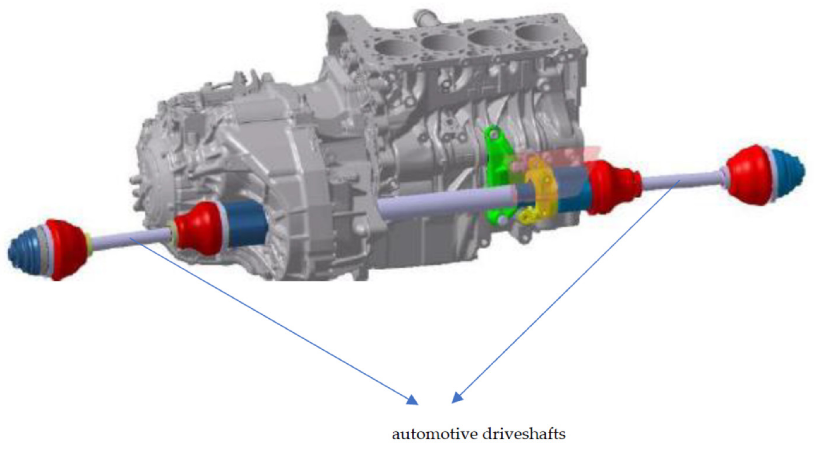
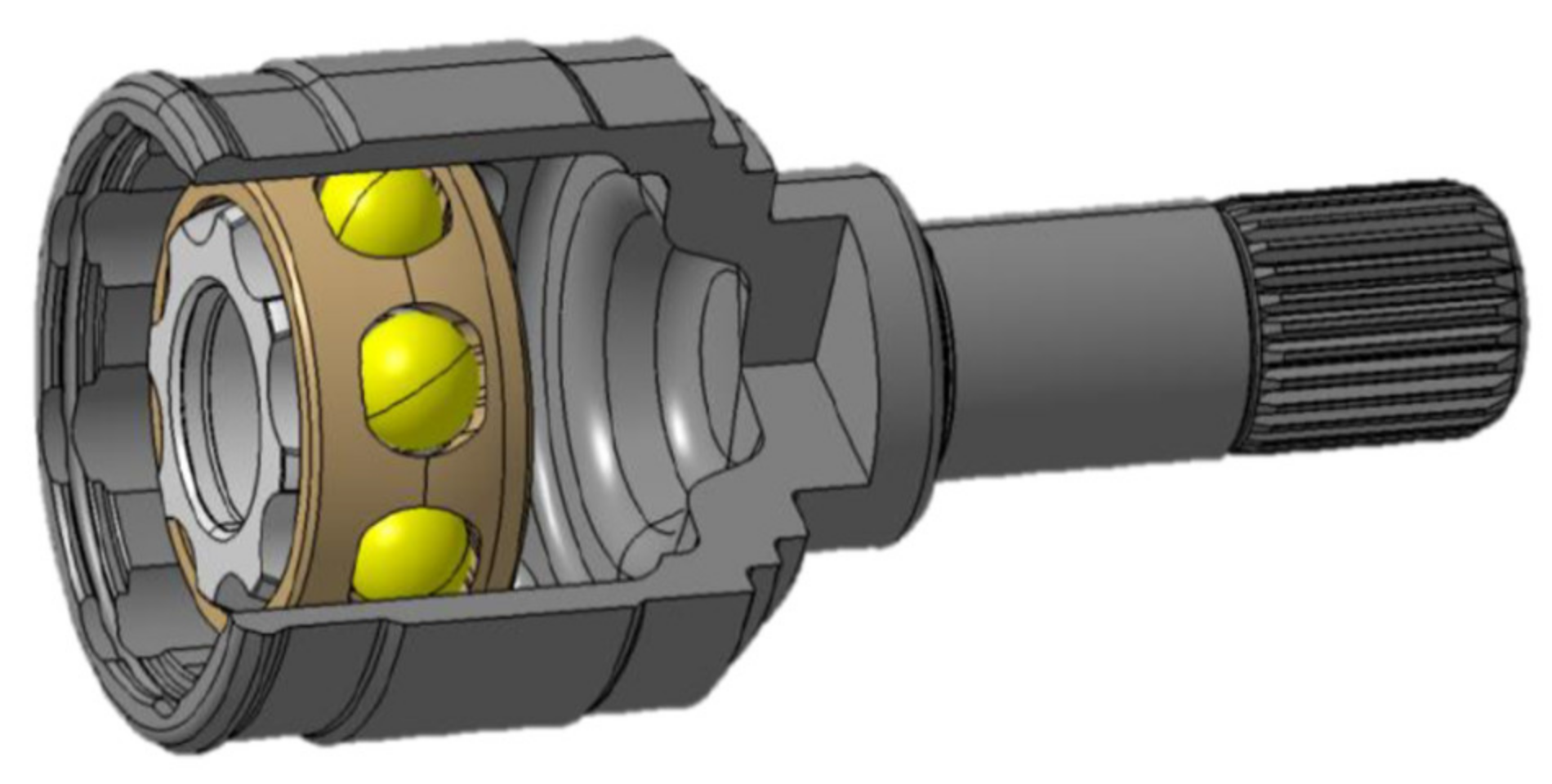
18] performed a detailed investigation of the vibration characteristics of the composite AD using the finite element method (FEM). This paper aims to investigate the dynamic behavior of the AD elements for the FBV movements in the PPR region. This investigation supposes the design of a model for FBV movements for an AD’s elements, the computation of the stationary and nonstationary amplitude spectrum in the PPR region, and the analysis of the dynamic instability frontiers in the same area. The novelty for this investigation is the design of the model of FBV movements of the AD elements and the use of a perturbation approach (AMA) to compute the amplitude, the phase angle, and the dynamic instability frontiers for both stationary and nonstationary motions. The designed model for FBV movements for an AD’s elements contains the phenomena of geometric inertia nonuniformity of the AD and the shock excitation of the AD due to the road geometry. An AD is a multibody mechanical structure mechanism that allows transmitting a moment from the gearbox to the wheel, as shown in
Figure 1. The principal components of such an AD, designed for heavy-duty SUVs, are presented in
Figure 2 and consist of the bowl (a) fixed with the steering wheel and the midshaft (b) that links both the bowl and the tulip (c).
The elements of the tulip–tripod joint is presented in
Figure 3, where the elements include the midshaft (a), on which the tripod (b) is mounted through the splines and linked with the tulip’s bell (c), and the tulip ax (d), which is fixed in the gearbox through the splines.
The elements of the bowl–inner race joint can be seen in detail in
Figure 4, showing the midshaft (a) on which is mounted the inner race (b) is fixed through splines, linked with the bowl’s bell (c), and the bowl ax (d) that is fixed to the steering wheel through the splines.
2. Computation of the Inertial Characteristics of the AD Elements for the FBV Movements
To use the AMA, it is necessary to compute the equations of the FBV movements for the AD elements, so it must be established from the beginning the movements of each AD element. Therefore, it was considered that the tulip and the bowl had deflections and rotations specific to the rigid body movements. In contrast, the midshaft had continuous deflections and rotations typical to a continuous elastic beam. These assumptions agreed with the technical reality because the rigidity of the tulip and the bowl are more significant compared with the midshaft’s rigidity. Each AD element has its referential system, presented in
Figure 5, namely the cartesian systems
.
The planes
are coplanar planes, so the axes
are parallel, and the movements considered for each AD element for the FBV movements are as follows (see
Figure 5):
- -
The rigid torsion rotation angles concerning the axes for the tulip, midshaft, and bowl;
- -
The rigid deflections in bending concerning the axes for the tulip and bowl;
- -
The rigid twisting angles in bending concerning the axes for the tulip and bowl;
- -
The rigid rotation angle of the tulip axis concerning the midshaft axis ;
- -
The rigid rotation angle of the bowl axis concerning the midshaft axis ;
- -
The elastic deflection in bending concerning the midshaft axis ;
- -
The elastic twisting angle in bending concerning the midshaft axis .
To compute the equations of the FBV movements of the AD elements using Hamilton’s principle, it was necessary to reduce the mass and geometric moments of inertia of the tulip and bowl to the cartesian system of reference of the midshaft
using the variation of the geometric moments of inertia concerning the concurrent axis and parallel axis (Steiner’s theorem). The geometric tulip’s design (see
Figure 3) is composed of the tulip’s bell (TB) and tulip ax (TA), while the geometric bowl’s design (see
Figure 4) is composed of the bowl’s bell (BB) and bowl ax (BA). The geometric and mass moments of inertia for the tulip
,
reduced to the
axes of the midshaft are given by the following equations:
where
are the principal geometric moments of inertia for the tulip’s bell,
are the geometric moments of inertia for the tulip’s elements reduced to the axes
,
is the mass density of the AD elements,
is the distance between the center mass of the tulip and the tripod’s center mass,
is the surface of the cross-section for the tulip’s bell,
is the nonuniformity of the geometric moments of inertia for the tulip (see
Figure 3),
is the length of the tulip’s bell,
is the length of the tulip ax, and
is the diameter of the tulip ax. The geometric and mass moments of inertia for the bowl
,
reduced to the
axes of the midshaft are given by the following equations:
where
are the principal geometric moments of inertia for the bowl’s bell,
are the geometric moments of inertia for the bowl’s elements reduced to the axes
,
is the distance between the center mass of the bowl and the inner race’s center mass,
is the surface of the cross-section for the bowl’s bell,
is the nonuniformity of the geometric moments of inertia for the bowl (see
Figure 4),
is the length of the bowl’s bell,
is the length of the bowl ax, and
is the diameter of the bowl ax. By analyzing Equations (1)–(18), it can be remarked that the geometric and mass moments of inertia of the tulip and the bowl, reduced to the referential of the midshaft, are functions of the angles
, meaning that they depend on the dynamic behavior of the tulip and the bowl, with this aspect being a novelty in designing dynamic models for the AD elements’ movements.
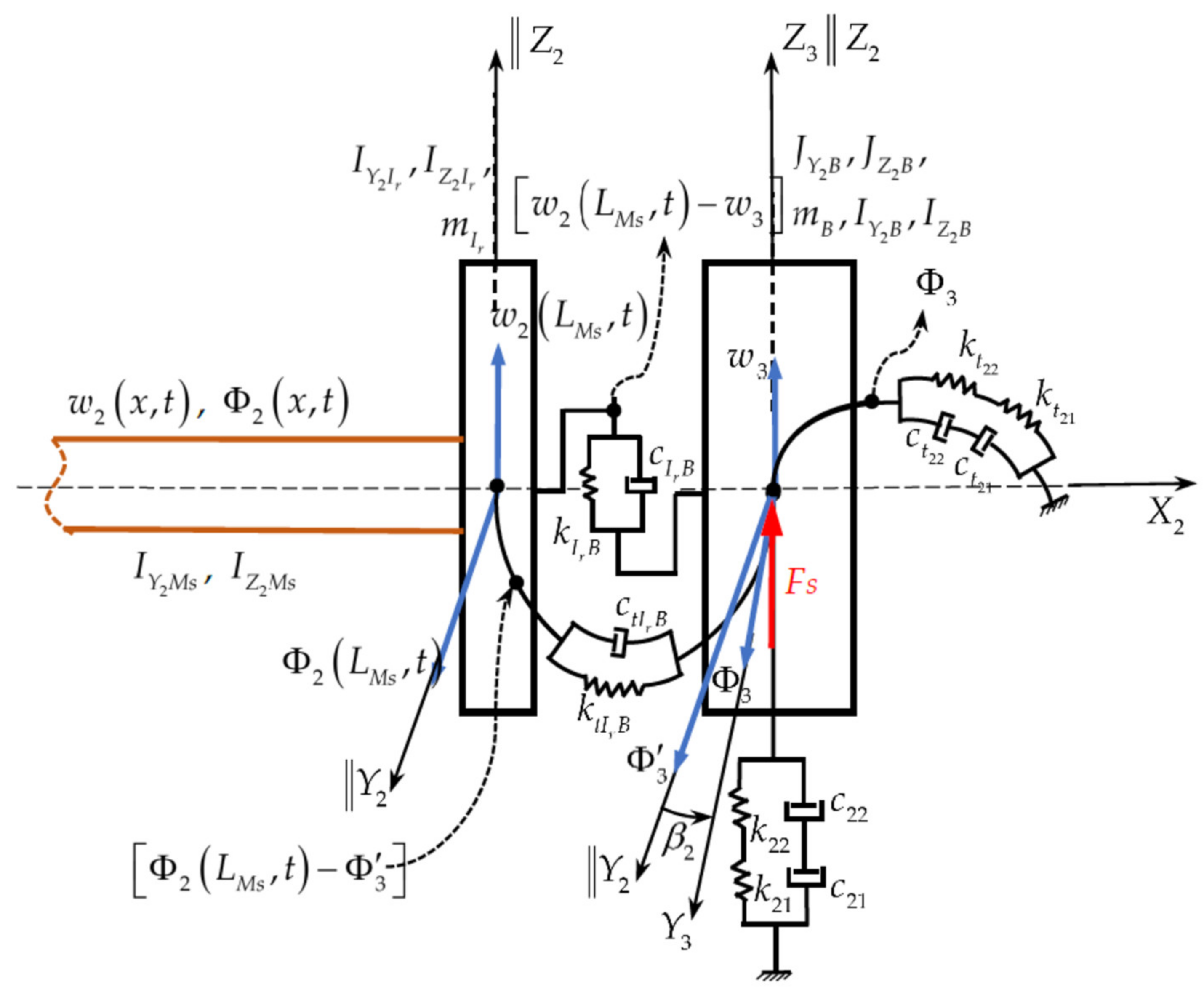
3. The Dynamic Model for FBV Movements of an AD’s Elements
The dynamic model for the FBV (DMFFBV) movements of an AD’s elements is presented in
Figure 6 and
Figure 7.
By surveying the literature already presented in the introduction, it can be remarked that there has not been detailed research performed for the dynamic behavior of each AD element. The dynamic model enhanced by the present work allows the investigation of the dynamic behavior of each component of the AD, the internal mechanisms of excitation transmissions through the AD elements, as well as the causes of producing pitting and micro-cracks in the AD elements, as revealed by the experimental data in the literature [
4] (pp. 88–94). The DMFFBV movements, presented in
Figure 6 and
Figure 7, have three elements: a tulip–midshaft–bowl linked through two joints, the tulip-tripod joint (mounted on the midshaft (see
Figure 3)), and the bowl–inner race joint (mounted at the other edge of the midshaft (see
Figure 4)). These have the following dynamic characteristics:
1. The tulip has a stiffness
, given by the serial springs
(see
Figure 6), and damping
, given by the serial dampers
, for the bending vibration rigid movement of the tulip regarding the axis
and a stiffness
, given by the serial springs
, as well as damping
, given by the serial dampers
, for the angular bending vibration rigid movement of the tulip regarding the axis
, given by the following relations:
where E is Young’s modulus, G is the shearing modulus,
is the tulip’s mass, and
is the logarithmic decrement of the free bending vibrations of the tulip (
= 0.001–0.01) [
19,
20].
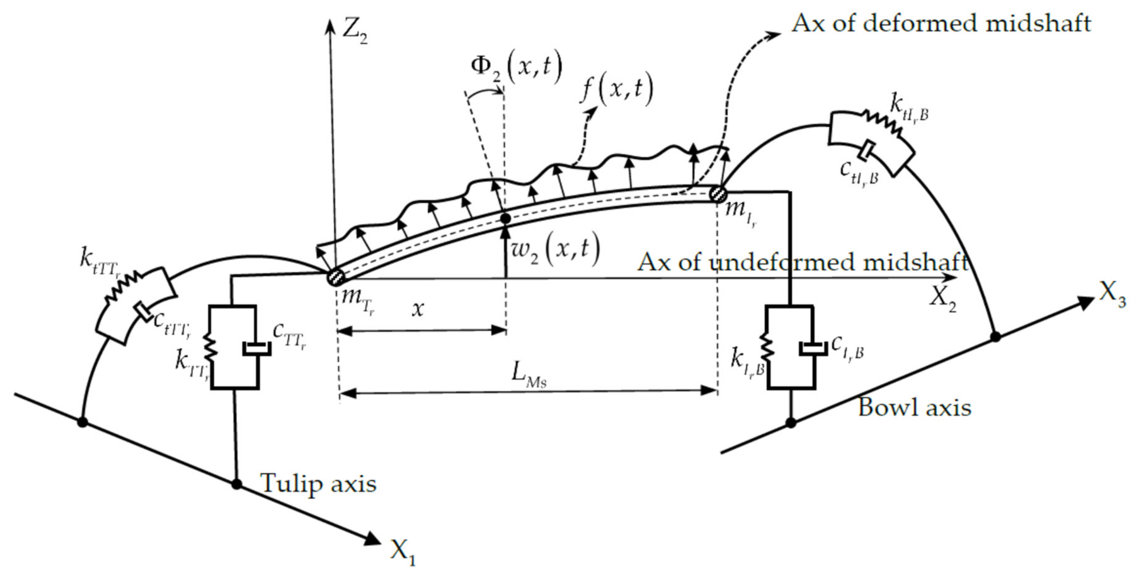
2. The uniform midshaft (see
Figure 2,
Figure 3,
Figure 4,
Figure 5,
Figure 6 and
Figure 7) in continuous FBV movement is assimilated with a uniform Timoshenko beam simply supported at both ends by elastic supports (the tulip-tripod and inner race-bowl joints are elastic supports for the midshaft), having at
a tripod (see
Figure 3) fixed on the midshaft through splines and elastically linked in the tulip-tripod joint with the tulip (see
Figure 6) and on the left-hand side at
an inner race (see
Figure 4) fixed on the midshaft through splines and elastically linked in the bowl-inner race joint with the bowl (see
Figure 7), with the inertial characteristics given by the relations below:
where
are the principal geometric moments of inertia for the tripod,
are the principal geometric moments of inertia for the inner race,
and
are the geometric nonuniformities of the tripod and inner race, and
are the geometric moments of inertia of the tripod and inner race concerning the axes
;
3. The bowl has a stiffness
, given by the serial springs
(see
Figure 7), and damping
, given by the serial dampers
, for the bending vibration rigid movement of the bowl regarding the axis
and a stiffness
, given by the serial springs
, as well as damping
, given by the serial dampers
, for the angular bending vibration rigid movement of the bowl regarding the axis
, given by the following relations:
where
is the bowl’s mass.
4. The tulip–tripod joint in FBV movement (see
Figure 3 and
Figure 6) realizes the elastic link between the tulip and the midshaft through the stiffness
and the damping
for the bending vibrating movements concerning the Z
2 axis and the angular stiffness
and angular damping
for the bending vibrating movements concerning Y
2 axis.
5. The bowl–inner race joint in FBV movement (see
Figure 4 and
Figure 7) realizes the link between the bowl and the midshaft through the stiffness
and the damping
for the bending vibrating movements concerning the Z
2 axis and the angular stiffness
and the angular damping
for the bending vibrating movements concerning the Y
2 axis. The wheel induces excitations as a moderate impulsive shock force F
s acting in the Z
2 direction, and the excitation load can be expressed as
where
is the amplitude of the shock on the bowl’s longitudinal axis
transmitted from the wheel axis and
are experimental constants, depending on the type of shock applied at the wheel by the road excitation [
4] (pp. 142–172). All the computations were performed considering that the tulip was a cantilever beam fixed in the gearbox with simple elastic supports in the tulip–tripod joint. The bowl was a cantilever beam fixed in the steering wheel by simple elastic supports in the bowl-inner race joint. As mentioned in the literature [
4] (pp. 142–172), the shock excitation loads produce huge automotive stress solicitations in the car suspension system and the rim-tire system. These two systems can absorb 90% of the shock energy. Therefore, only 10% of the shock acts on the AD elements as a variation of the quantity of movement during a very short time, estimated at 0.001 s. Because of this phenomenon, the shock is distributed to each AD element, inducing for the bowl stress in the region of the splines, for the midshaft the initial velocity of the “ends”, and for the tulip stress in the region of the splines (see
Figure 2). Due to this mechanism of excitation, it will be considered that the stress in the tulip’s ax and bowl’s ax imposes the geometric capability dimensions of the geometric elements
. At the same time, the midshaft dynamic behavior will be an excitation element, like the internal tuned damper (ITD) mentioned in the literature [
6], for the tulip and the bowl. The novelty of this DMFFBV of an AD’s elements, as can be noted from Equations (19)–(25), consists of linking the rigid movements of the bowl and the tulip with the continuous movement of the midshaft. In addition, another novelty is that the dynamic characteristics concerning stiffness and damping are expressed for the bending displacements and the bending rotation displacements for each AD element, and the serial stiffness and damping of the bowl and tulip are considered, keeping in mind that each of these elements has two distinctive parts: the ax and “bell”. In the meantime, the stiffness and damping for the tulip-tripod and bowl-inner race joints were considered for the relative bending displacements and the relative bending rotation displacements of the movements between the bell of the tulip and the tripod, as well as for the inner race and the bell of the bowl.
4. The Equations of FBV Movements of AD Elements Induced by Shock Road Excitations
For the DMFFBV movements of AD elements presented in
Figure 6 and
Figure 7, using the Hamilton’s principle [
21] (pp. 265–269) yields
where Lagrange’s function
depends on the generalized coordinates
and the generalized velocities
, while
are two points in the spatial configurations
. Lagrange’s function is given by the following equation:
where the potential energy
for the DMFFBV movements of AD elements (see
Figure 6 and
Figure 7) is given by the following generalized equation [
22] (pp. 371–376) [
23] (pp. 734–739):
where A is the cross-section area of the midshaft,
is the bending deflection (including the shear deformation) of the midshaft concerning the
axis, Φ
2 (x, t) is the rotation of the cross-section of the midshaft, and concerning the
axis, due only to the pure bending deflection,
is the shear correction factor, which in the literature [
24] is in the range of 0.64–0.846,
is the length of the midshaft, and
is the geometric moment of inertia of the midshaft concerning the
direction given by the following equations:
where the midshaft is considered to have a circular or tubular uniform cross-section with a diameter
for the circular cross-section or the diameters
for the tubular cross-section. In Equation (28), the generalized Rayleigh’s dissipation function [
23] (p. 611) specific to the mathematical formulations of the Euler–Lagrange generalized approach was added due to the presence of dampers in the DMFFBV movements, given by the following equation:
The kinetic energy of the DMFFBV movements (see
Figure 6 and
Figure 7) for an AD’s elements is given by the following generalized equation [
22] (p. 374) [
23] (p. 721):
where
is the mass of the tripod and
is the mass of the inner race (see
Figure 6 and
Figure 7). Several mathematical manipulations that include integration by parts of the nonlinear system of equations with partial derivatives of the second degree in the unknowns
and
, yield
where the boundary conditions are
Taking into account that the tulip was fixed in the gearbox (see
Figure 6 on the left side) and had simple elastic supports in the tulip-tripod joint (see
Figure 6), the midshaft was a uniform Timoshenko beam simply supported by elastic at both ends (see
Figure 6 and
Figure 7) in both the tulip-tripod (left side) and inner race-bowl joints (right side), while the bowl was fixed (see
Figure 7, right side) in the steering wheel and had simple elastic support in the inner race-bowl joint (see
Figure 7). The system is given by the Equations (33)–(38) together with the boundary conditions from Equations (39)–(44) to represent the nonlinear dynamic behavior of the AD elements in FBV induced by shock force through the wheel by road excitations. By analyzing Equations (35) and (36), it can be remarked that they represent a system of equations with partial derivatives for the bending-shearing vibrations of a uniform shaft that considers the effects of rotary inertia and shear deformation, with the midshaft being a Timoshenko beam. The boundary conditions are given by Equations (39)–(44) and link the bending-shearing vibrations of the midshaft with the tulip and the bowl through the tulip-tripod and bowl-inner race joints, inducing in the solutions of the system of Equations (33)–(38) the next phenomena: the joints of the driveshaft are quasi-isometric [
25,
26,
27] (p. 78), with the effect of geometric nonuniformity of the inertia characteristics of the joints that vary with the rigid angle of rotation for each element of the driveshaft in the directions
the effects of the bending deflection and bending-twisting stiffness for the tulip and the bowl, the effects of the bending deflection and bending-twisting damping for each joint of the driveshaft, the rotary inertia effect in bending, and the shearing effect for the midshaft. The novelty of the Hamilton’s Principle approach was that it was used for the first time to compute the equations of motion for each AD element and the determination of the boundary conditions, as is noted in Equations (26)–(44).
5. The Analytical Solutions
The starting point to solve the system differential equations of the FBV movements (SDEOFBVM) (Equations (33)–(38)) for the AD elements (ADEs) was to analyze the vibration mechanism of the midshaft as a Timoshenko beam simply supported at the ends (see
Figure 8 and
Figure 9). For the midshaft element of the AD, it was considered that
In analyzing the tulip-tripod-midshaft and bowl-inner race-midshaft joints, it became evident that the midshaft was simply supported at both ends where the concentrated mass of the tripod and the inner race
were placed, being a uniform shaft linked in bending-shearing vibration with the tulip for x = 0 and with the bowl for x = L
Ms. Therefore, the general solutions of Equations (35) and (36) that satisfy the boundary conditions of Equations (39) and (40) expressed in normalized bending deflection are [
23] (pp. 326–328)
where
are the natural frequencies of the Timoshenko beam simply supported at both ends [
23] (p. 378), the smaller value corresponds to the bending deformation mode, and the bigger value corresponds to the shear deformation mode, given by the following equation:
Additionally, the constants
are determined by the initial conditions at t = 0. In our case, the constants are given by the equation [
4] (pp. 142–172)
where
is the time interval for shock excitations due to the road geometry and M is the car’s mass. Injecting the solutions given by Equations (45) and (46) in the boundary conditions of Equations (41) and (42) yields the following boundary conditions for the tulip and the bowl in bending:
Equations (49) and (50) can now be injected in Equations (33) and (37) for the DMFFBV, thus yielding DMFFBV equations for the tulip and bowl:
Taking into account that Browne and Palazzolo in [
6] mentioned that excitation terms, as presented on the right side of Equations (51) and (52) could be expressed as cubic internal tuned dampers (ITDs), the forms of Equations (51) and (52) can be modified by dividing Equations (51) and (52) into the mass of the tulip
and the mass of the bowl
, respectively, expressing the stiffness and damping coefficients as functions of the geometrical characteristics given by Equations (19) and (23) coupled with the expressions of inertial characteristics provided by Equations (8), (9), (17), and (18). Equations (51) and (52) become the normalized differential equations in the time functions
:
where the coefficients
are presented in
Appendix A, and the damping ratio
is given by the following equation:
The natural frequency of the tulip in bending
and the natural frequency of the bowl in bending
are given by the following equations:
The coefficients of the cubic and quintic terms expressed in Equations (53) and (54) can be mathematically explained by development in a Taylor infinite series induced by the excitation function
(see Equations (53) and (54)) expressed approximately as
In the PPR region, the excitation terms
and
must satisfy the Equations (59) and (60), as mentioned in [
28] (p. 425), since this resonance is one of the most important, as mentioned in [
5,
6,
28]:
where
is the excitation frequency in the PPR region for the tulip,
is the excitation frequency in the PPR region for the bowl,
is the excitation induced in the FBV movement (Equation (53)) by the rigid twisting angle of the tulip concerning the
axis, and
is the excitation induced in the FBV movement (Equation (54)) by the rigid twisting angle of the bowl concerning the
axis, as given by the following equation:
This considers the nonuniformity of the kinematic isometry of the AD [
25,
26]. In Equation (61), the terms
represent the radii of the tulip-tripod and inner race-bowl joints. Considering the conditions imposed by Equations (59) and (60) together with Equation (58) and Equations (48)–(50), the coefficients of the cubic and quintic excitation terms on the right-hand side of Equations (53) and (54) are
By analyzing Equations (53) and (54), they are a generalized form of Mathieu–Hill nonlinear equations coupled through Equation (61), describing the FBV movements of the tulip and the bowl induced by shock excitations due to the road geometry. These equations contain the following phenomena: the non-uniformity of geometric and kinematic isometry of the AD, the non-uniformity of the inertial characteristics for the tulip and the bowl and forced shock excitations due to road excitations. By analyzing the initial system of Equations (33)–(38) with the boundary conditions of Equations (39)–(44), it can be seen that Equations (34) and (38), together with the boundary conditions of Equations (43) and (44), were not used in the mathematical procedure solution because these equations represented the nonlinear dynamic behavior of the FBV angular shearing movements of the AD (the AD’s elements of the tulip, midshaft, and bowl), and the present article is dealing with the nonlinear dynamic behavior of the FBV deflection movements of the ADE, namely the bowl, midshaft, and tulip. The FBV movements of the midshaft have the solution given by Equation (45) coupled with Equations (47) and (48). In contrast, the shearing FBV movements of the midshaft have the solution given by Equation (46) coupled with Equations (47) and (48), both representing the solution of Equations (35) and (36) from the SDEOFBVM (Equations (33)–(38)), with the boundary conditions of Equations (39) and (40) from the general system of Equations (39)–(44) that imposed the boundary conditions. Additionally, it is noted that for the nonlinear dynamic behavior of the AD, the dynamic behavior of the midshaft represents an excitation-like internal tuned damper (ITD) used by Browne and Palazzolo in the superharmonic nonlinear lateral vibrations (forced bending vibrations) of an AD [
6]. This aspect represents a novelty in the investigation of the dynamic behavior of the ADE, because it allows for the computation of the equations of motion for the tulip and the bowl in a mathematical form adequate for performing a perturbation approach, as can be seen from Equations (53) and (54). Another aspect of this novelty is the capability of computing the natural free frequency in bending for the tulip and the bowl (see Equations (56) and (57)) and to express the excitation frequency in the PPR region, as is noted from Equations (59) and (60). In the meantime, a supplementary aspect of the novelty is the estimation of the shock excitation of the road geometry as cubic and quintic excitation terms in the equations of motion, as is shown by Equations (56) and (57) and the relations of Equations (62) and (63). For the first time, the effect of the nonuniformity of the kinematic isometry of the AD was considered, being expressed by Equation (61), which links the equations of motion for the FBVM regarding the tulip and the bowl.
6. Analysis of the PPR Region for the Tulip and Bowl
As already mentioned above, one of the most important resonant cases of an AD is the PPR [
5,
6], [
28] (p. 425), and for this paper, the authors decided to investigate the dynamic behavior of FBV movement in the PPR region for the tulip and the bowl based on Equations (53) and (54). Similar experimental data for this case study are presented in the literature by Steinwede [
4] (pp. 69–144). The study considered a tulip having geometric characteristics such as the geometric moment of inertia and nonuniformity of the geometric moments of inertia, as presented in
Table 1 [
29], for the tulip AD element. By comparing these presented geometric characteristics with those considered by Steinwede [
4] (p. 111), it can be concluded that there is agreement. Using AUTOCAD software,
were computed based on the direct geometric characteristics
and the general geometry of the tulip.
It can be remarked that the nonuniformity of the inertial geometric characteristic
in
Table 1 had another value than what was considered in literature because of the geometric characteristic in the cross-section of the tulip presented in
Figure 9.
Table 2 presents the physical properties of the material of the tulip and the amplitude and duration of the shock, considering that the material was steel and iron cast. By comparing these presented material properties with those considered by Steinwede [
4] (p. 112), it can be concluded that they were in very close agreement.
To compute the amplitude of the FBV movements of the ADE tulip in the PPR region using a perturbation approach, several methods could be used: the method of harmonic balance [
29] (p. 66), the asymptotic method [
1] (pp. 299–393), or the method of multiple scales [
28] (pp. 424–427). The method of harmonic balance is very efficient, as mentioned in the literature [
30] (p. 63), [
31], but it allows the computation of the amplitude versus the frequency excitation only for stationary (steady state) motion without the possibility of computing the phase angle [
30] (pp. 63–68). Therefore, this method is limited to the steady state FBV. The multiple scales method is challenging to use due to the conditions of zeroing the secular term and the additional necessary study of the convergence of the detuning parameter. Considering these aspects, the authors chose to use the AMA in the first-order approximation. This would allow the investigation of the amplitude and phase angle versus the excitation frequency for the FBV movement of the tulip in the PPR region for both the stationary and nonstationary cases. To compute the solution of Equation (53), it was assumed that the slowing time was
, where ε is a small positive parameter [
1] (p. 299). To introduce the slowing time, Equation (53) needed to be transformed to be used in the AMA. The coefficients of the second and third term of Equation (53) on the left side can be expressed as
where in Equation (64), the condition given by Equation (59) was considered. With the relations in Equation (64), Equation (53) becomes
The assumption that the damping ratio
, the excitation coefficient
, and the coefficients of cubic and quintic nonlinearity
are small is incorporated in the analysis by representing these quantities in the following form:
where ε is the same small positive parameter used to obtain the slowing time. It is also assumed that the excitation frequency
and the excitation parameter
vary slowly with time, such that
Equation (65) becomes the following after neglecting the terms in
:
Regarding Equation (68), the right-hand side represents a perturbation of the mathematical form
, being a periodic function in
with period 2π, while the left-hand side of the equation is a linear oscillator. By considering all these physical considerations and confining our attention to the investigation of the PPR region, a solution for Equation (68) is sought after in the following form to the first-order approximation in
:
where
and
are functions of time defined by the system of differential equations:
Differentiating the right-hand side of Equation (70) and expanding the results in powers of ε yields
When differentiating the right-hand side of Equation (69) while considering the systems of Equations (70) and (71) and retaining only the first-order terms, we obtained the following:
Using Equations (72) and (73) in the basic form of Equation (68), equating the terms of the form
from the left-hand side of Equation (68) with the same terms from the right-hand side of the same equation and neglecting the overtones (the terms having
) yields the two following coupled first-order differential equations for the unknown functions A
1 and B
1:
This system of Equations (74) and (75) has the following solutions:
By introducing the solutions of Equation (76) into the system of Equation (70) and transforming all the system parameters back to their real-time values, the solution of Equation (65), representing the FBV movement of the tulip in the PPR (
) is given by Equation (69) using the first-order approximation of the AMA, where the amplitude W and the phase angle ψ are given by integrating over time the first-order differential system:
6.1. Steady State Forced Bending Vibration of the Tulip
For the stationary FBV movement for the tulip of the AD, it would be set to zero
and
in Equation (77), and expressed from these equations,
and
yields the trigonometric equation
expressing in terms of the system in Equation (77) the bi-quartic equation in the unknown W the amplitude versus the excitation frequency:
where the coefficients λ
5–λ
9 are given in
Appendix A. The solutions to Equation (78) represent the stationary amplitude of the forced bending vibration of the tulip in the PPR region. The stationary phase angle of the FBV movement for the tulip in the PPR region is given from the same system (Equation (77)) set to zero by expressing the tangent of the phase angle, yielding
6.2. Investigation of Dynamic Instability
The investigation of the dynamic instability of the FBV movement for the tulip represents the computation of the boundaries of the principal parametric region of instability. The base width of the stationary response is the only region in which vibrations may typically initiate. Setting to zero the amplitude in Equation (78) yields the following equation:
Alternatively, it may yield
Equation (81) gives the boundaries of the principal parametric region of instability in the space . This is the investigation for the stationary FBV movement of the tulip. For the nonstationary FBV movement of the tulip, the investigation of the dynamic instability consisted of the analysis of the spectral graphs of the nonstationary amplitude and the first derivative of the nonstationary amplitude concerning time, given by the integration of the system of Equation (77). The graphed representation in the configuration space of the “speed” nonstationary amplitude versus the nonstationary amplitude is evidence of the transition of FBV movement for the tulip through the chaotic movement in the PPR region, and the results are presented in the next paragraph.
6.3. Nonstationary FBVM of the Tulip and Bowl during Transition through the PPR
The resonant regimes of the principal parametric vibration for the forced bending vibration of the tulip were determined. It may be of interest to examine the nature of the nonstationary vibrations performed by the system during a transition of the excitation frequency
through the resonant regime. For this purpose, it was necessary to integrate the system of Equation (77) governing the nonstationary amplitude and the phase angle. This system of differential equations cannot be integrated into the closed form, and therefore, it was obvious to use numerical integration. It may be pointed that numerical integration of first-order equations governing the stationary amplitude and phase angle versus frequency excitation is a much simpler process than the integration of the original system of Equation (77), which is nonlinear since it must evaluate the envelope of an oscillatory function and not the function itself. In the present nonstationary analysis, the sweep of the excitation frequency is taken to be logarithmic and is expressed as
where
is the initial frequency at t = 0 for the tulip and m is the sweep rate (in octaves/min). The differential system of Equation (77) is integrated numerically using a fourth-to-fifth order Runge–Kutta algorithm from the MATLAB software with a variable integration step of the prediction-correction type. The initial values of the variables W,
, and
were chosen as a stationary state starting point. The investigation of the nonstationary forced bending vibration of the tulip was confined to the PPR region, and the results are presented in the next paragraph. For the bowl, the analysis of the PPR region was based on Equation (54) for FBV movement (FBVM), with the excitation frequency
given by Equation (60), the natural frequency
established by Equation (57), the cubic and quintic terms
given by Equation (63), and the excitation coefficient being
while the terms
are presented in
Appendix A. For the investigation of the nonstationary FBVM of the bowl, the system of differential equations is from Equation (77), using the excitation frequency
, the natural frequency
, and the cubic and quintic terms
, while the rate of sweep m is established as
where
is the initial frequency at t = 0 for the bowl.
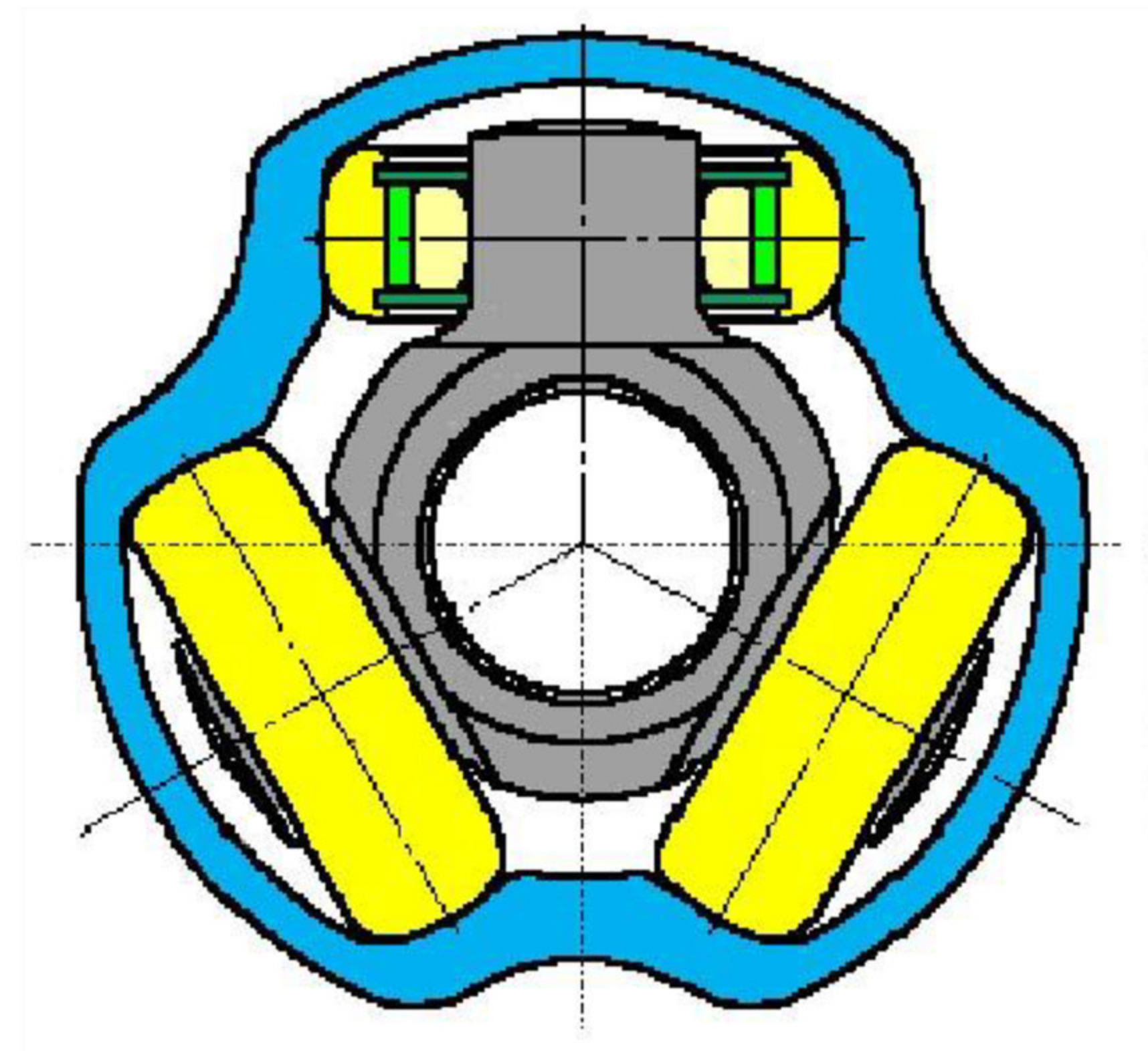
Table 3 presents the geometry and inertial characteristics of the bowl. Using AUTOCAD software,
were computed based on the direct geometric characteristics
and the general geometry of the tulip. The material’s physical properties are the same as those presented in
Table 2.
Figure 10 presents the axonometric cross-section of the bowl.
When comparing these presented geometry characteristics (see
Table 3) with those considered by Steinwede [
4] (p. 112), it can be concluded that they agree. The novelty for investigating the PPR region of an AD is that the AMA was used for such a multibody technical system for the first time. The AMA has no limitations on its use because it allows the development of analytical solutions for the amplitude, phase angle, and dynamic instability frontiers for stationary and nonstationary motion, as can be seen from Equations (65)–(83). Additionally, the AMA allows for significant precision for the computations because it can provide several levels of approximation. In our case, it was used for first-order approximation. For the first time, the amplitude, phase angle, and dynamic instability frontiers for the stationary motion of the FBV of a tulip and bowl in the PPR region were computed, as can be seen by analyzing Equations (78), (79) and (81). In the meantime, the amplitude spectrum, “speed” amplitude spectrum, and representation in the phase space
of the “speed” amplitude versus amplitude for the nonstationary motion in transition through the PPR region of the tulip and the bowl was determined for the first-time using Equations (77), (82) and (83).
7. Results and Discussion
The first results obtained were represented by the natural free frequencies in bending and shearing of the midshaft, given by Equation (56):
Based on Equations (56) and (83), the natural free frequencies of the midshaft in bending-shearing is an infinite series covering a wide range of frequencies, and thus by comparing the numerical results obtained with the mentioned equations and the experimental data and numerical data (using FEA-ANSYS) presented in the literature [
13] and analyzing the data presented in
Table 4, agreement for the bending natural free frequencies of the midshaft of the AD was found.
As can be seen from
Table 4, the agreement of the results was for the free bending natural frequency, while the second free natural frequency represents the free shearing natural frequency that, as can be noticed, was like the principal parametric resonance compared with the bending. This confirms that the designed DMFFBVM of the AD was much more reliable than the FEA-ANSYS and modal analysis presented in the literature [
13]. As mentioned in [
13], the dynamic forced vibration of the AD was inducing cracks in the AD’s structure, a fact also revealed by Steinwede [
4]. Additionally, it was mentioned in [
13] that experimental data were found for the midshaft, and this aspect revealed the fact that the midshaft had such a nonlinear dynamic behavior that represented the excitation element for the other components of the AD, namely the tulip and the bowl, playing the same role as the internal tuned damper (ITD) mentioned in the literature [
8] for the superharmonic nonlinear lateral vibrations (bending vibrations) of the AD. The fundamental natural free bending vibrations of the tulip given by Equation (56) was
, considering the geometrical characteristic and the physical properties presented in
Table 1 and
Table 2 for the AD designed for a heavy duty SUV, which conformed with the experiments of Steinwede that imposed an investigation of the forced torsional or bending vibrations of a driveshaft in the range of 0.5–15 kHz [
6] (p. 119). Unfortunately, no published experiments investigated the natural free frequency in bending only for the global tulip, midshaft, or global bowl. For the steady state FBV of the tulip and the bowl, specific MATLAB software was developed to compute the amplitude and phase angle in the region of principal parametric resonance based on Equations (78) and (79).
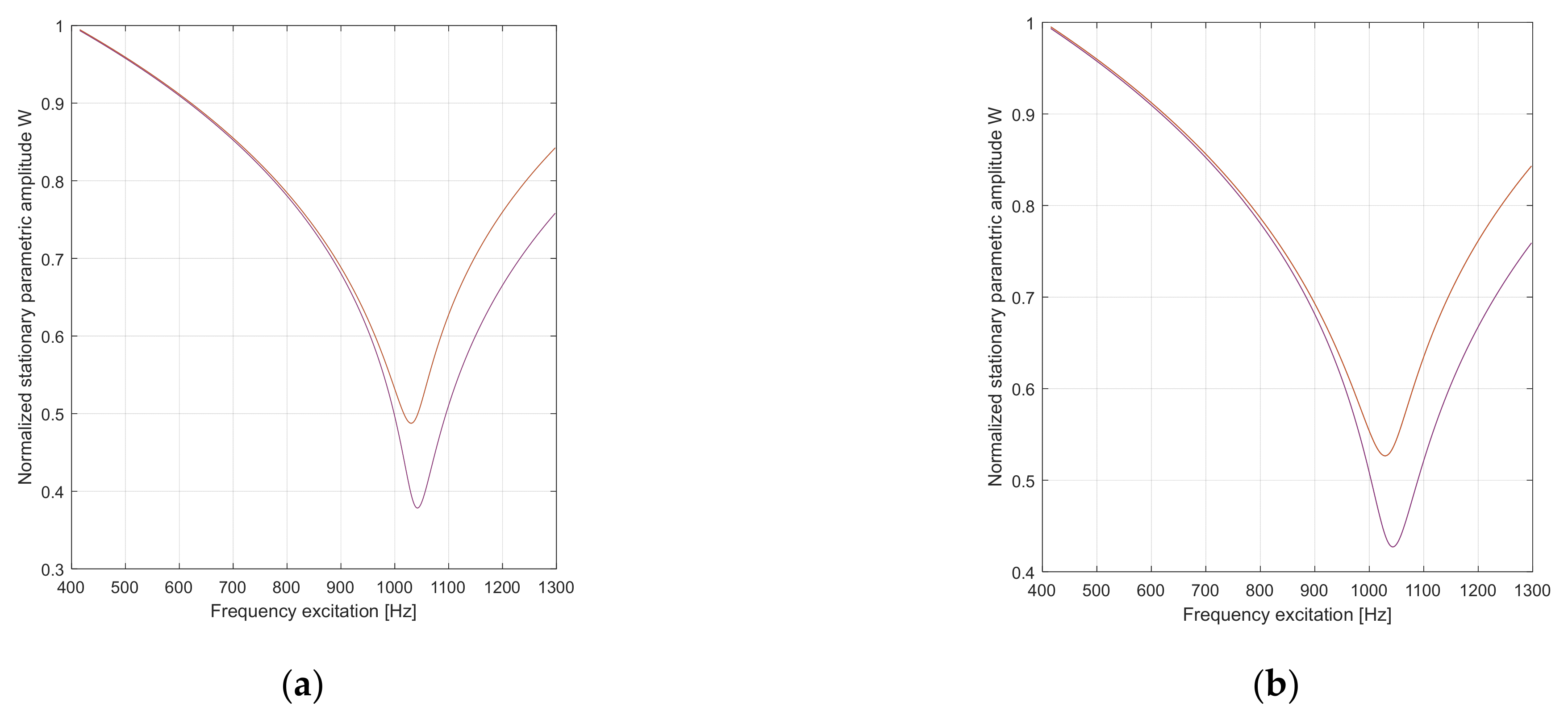
Figure 11 and
Figure 12 present the variation of the normalized stationary amplitude for the FBV in the PPR region for the tulip of an AD, with this being around 1038.38 Hz.
When analyzing the normalized stationary parametric amplitude presented in the graphs in
Figure 11 and
Figure 12 for
= 0.0016–0.0318 and
= 0.25, it can be found that for the cases, we had a manifestation of a “soft spring” with one branch for
that indicated the presence of interaction between the principal parametric resonance and the primary resonance, while for
, two branches of a “hard spring” existed, which suggests the manifestation of interaction with the combination resonance or with the internal resonance for the tulip [
28] (pp. 132–160). This aspect agrees with the experimental data in the literature [
4] (pp. 130–144). It can also be remarked that the increase in the damping ratio in the range of 0.0016–0.0318 increased the minimum normalized stationary amplitude from 0.13 to 0.42 for one branch, and for the second branch, the increase in the minimum normalized stationary amplitude was from 0.32 to 0.425. This can be explained by the existence of dynamic instability in the region of principal parametric resonance, as mentioned in the literature [
28] (pp. 132–160).
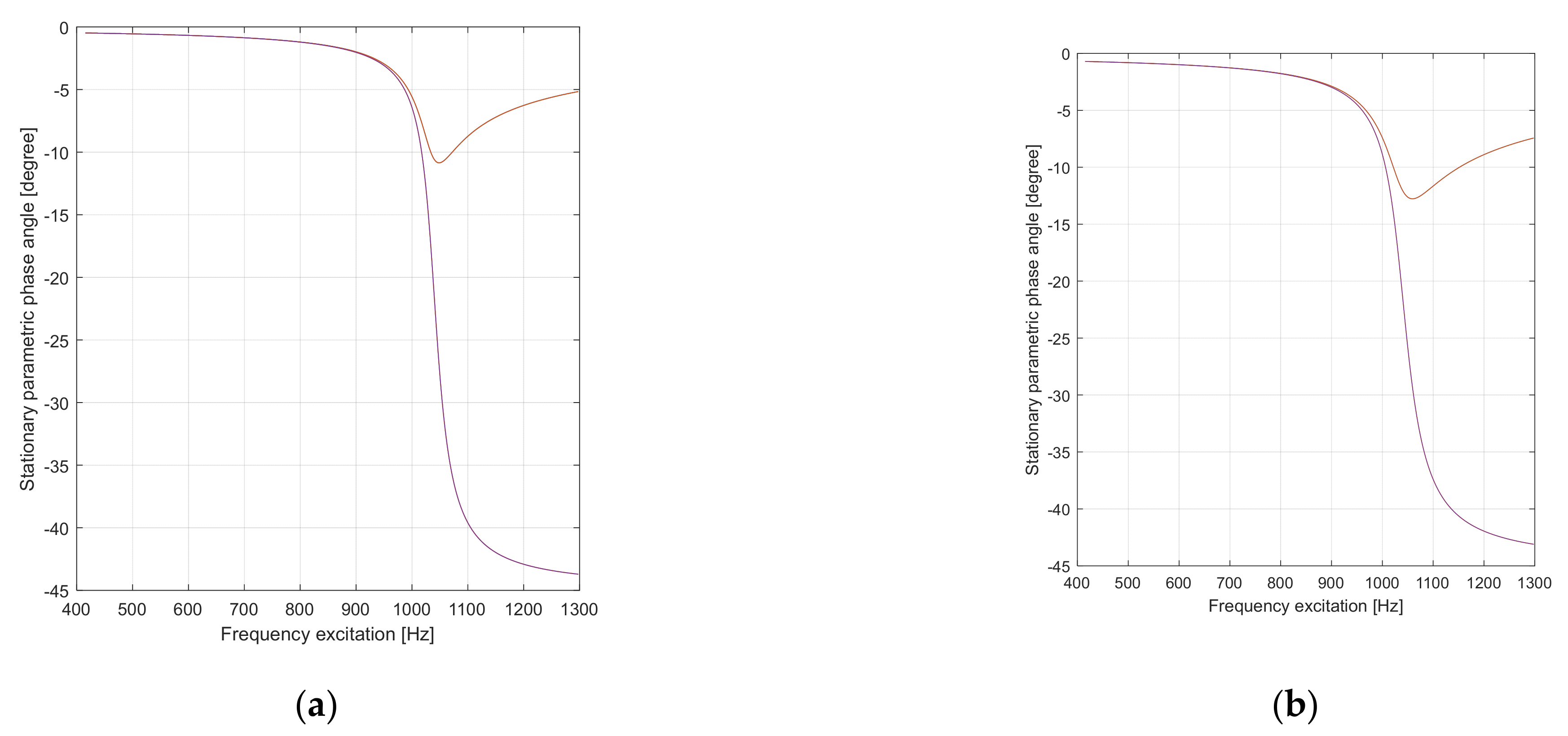
Figure 13 and
Figure 14 present the variation of the stationary phase angle for the FBV in the PPR region for the tulip of an AD.
When analyzing the stationary parametric phase angle presented in the graphs in
Figure 13 and
Figure 14 for ζ = 0.0016–0.0318 and
= 0.25, it can be seen that for the cases, we had a manifestation of a “soft spring” with one branch for
, while for
, two branches of a “hard spring” exist, but with the increase in the damping ratio passing through the principal parametric resonance for
, and in the region of a “hard” spring, the two branches are approaching one against the other. In addition, the manifestation of increasing the value of the minimum of the second branch was sensitive to the increase in the value of the damping ratio in the range mentioned above (0.0016–0.0318). Through experiments, Steinwede demonstrated that the nonlinear parametric dynamic behavior of automotive driveshafts is like that of geared systems [
4] (p. 117), [
32] (pp. 132–160), and therefore, we observed similar pitting phenomena as well as micro-cracks inside the tulip and the bowl of the CVJ tulip-tripod and bowl-inner race joints [
6] (pp. 88–94), which was also mentioned in the literature [
13]. These aspects will “conduct” dynamic behavior through a chaotic dynamic that has, as a practical effect, an accelerating effect on pitting phenomena and cracking, as mentioned by Steinwede [
4] (pp. 88–94) or, in the worst case, results in the manifestation of cracks followed by failure (breaking) of the tulip [
4] (p. 89).
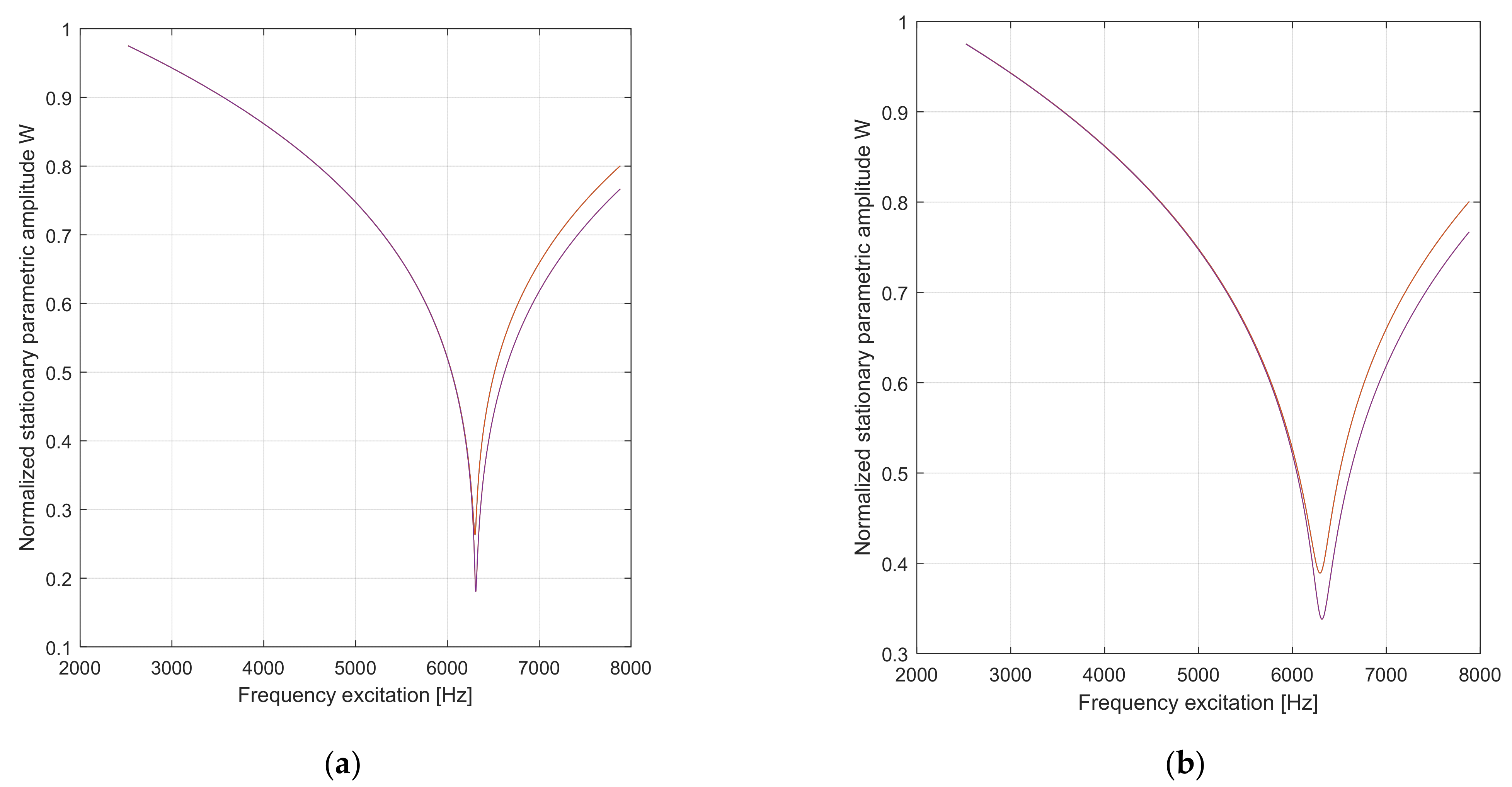
Figure 15 and
Figure 16 present the variation of the normalized stationary amplitude for the FBV in the PPR region for the bowl of an AD (around 6306.6 Hz). The fundamental natural frequency in bending for the bowl (3153.3 Hz) was computed with Equation (57). As can be seen, the natural frequency for the bowl was much bigger than the natural frequency of the tulip, and the PPR region for the bowl was in the PPR region for the forced torsional vibrations of the tulip, as mentioned in the literature [
29].
When analyzing the normalized stationary parametric amplitude of the bowl presented in the graphs in
Figure 15 and
Figure 16 for
= 0.0016–0.0318 and
= 0.10, the same manifestation in the PPR region for the bowl as for the tulip can be seen but in a different range frequency. The manifestation of a “soft spring” with one branch for
can be noted, indicating the presence of interaction between the principal parametric resonance and the primary resonance of the bowl, while for
, two branches of a “hard spring” existed, which indicates the manifestation of interaction with the combination resonance or with the internal resonance for the bowl [
28] (pp. 132–160). This aspect agrees with the experimental data in the literature [
4] (pp. 130–144). It can also be remarked that the increase in the damping ratio in the range of 0.0016–0.0318 increased the minimum normalized stationary amplitude of the bowl from 0.18 to 0.45 for one branch, and for the second branch, the increase in the minimum normalized stationary amplitude was from 0.29 to 0.49. This can be explained by the existence of dynamic instability in the region of principal parametric resonance, as mentioned in the literature [
28] (pp. 132–160).
Figure 17 and
Figure 18 present the variation of the stationary phase angle for the FBV in the PPR region for the AD bowl.
When analyzing the stationary parametric phase angle for the bowl presented in the graphs in
Figure 17 and
Figure 18 for ζ = 0.0016–0.0318 and
= 0.10, the same kind of manifestation as that for the tulip, but in a different range frequency, can be seen, and for the cases, we had a manifestation of a “soft spring” with one branch for
, while for
, two branches of a “hard spring” existed, but with the increase in the damping ratio, the passing through principal parametric resonance was found for
, and in the region of the “hard” spring, the two branches were approaching one against the other. For the bowl, this aspect of the two branches closing one against the other was more accentuated. Additionally, the manifestation of increasing the value of the minimum of the second branch was sensitive to the increase in the value of the damping ratio in the range mentioned above (0.0016–0.0318).
Figure 19a,b illustrates the stationary dynamic instability region of the tulip in the space
using MATLAB software and Equation (81). When analyzing
Figure 19a,b, it can be noticed that the two folded surfaces obtained were symmetrical concerning the plan given by
for the excitation frequency and the damping ratio. In contrast, the excitation coefficient
could be positive or negative. The folded surface of the dynamic instability “kept” inside the two branches the region where it manifested the stationary instability. It can also be seen that increasing the damping ratio had a stabilizing effect on the dynamics of the tulip, as expected.
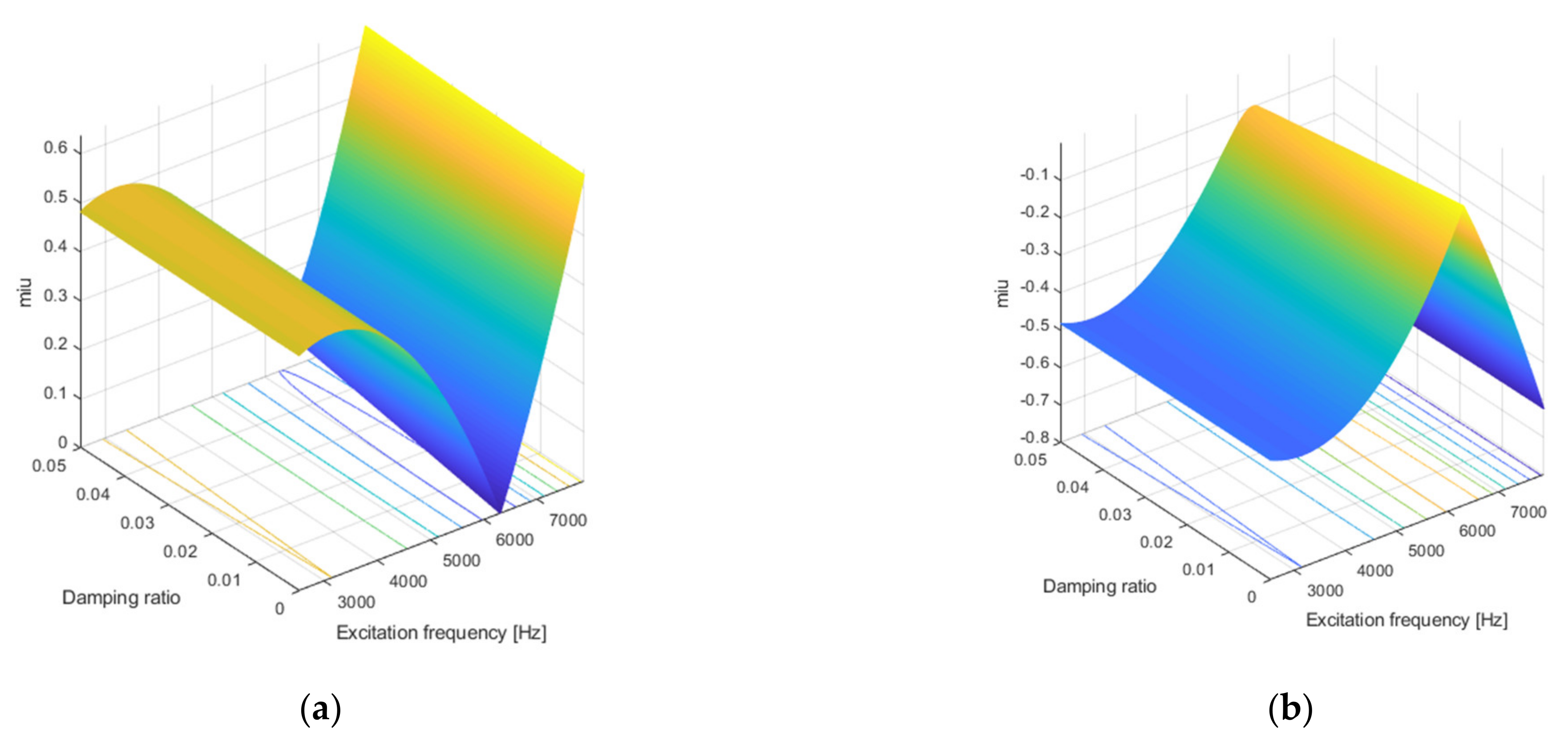
Figure 20a,b illustrates the stationary dynamic instability region of the bowl in the space
using MATLAB software and Equation (81).
By analyzing
Figure 20a,b, it can be noticed that the two folded surfaces obtained were symmetrical concerning the plan given by
for the excitation frequency and the damping ratio, while the excitation coefficient
could be positive or negative. The folded surface of the dynamic instability “kept” inside the two branches the region where it manifested the stationary instability for the bowl. It can also be seen that increasing the damping ratio had a stabilizing effect on the dynamic of the bowl, as expected. The only difference for these phenomena for the bowl was that the manifestation was in another range frequency than that of the tulip: the range frequency given by the natural frequency of the bowl in bending.
Figure 21 illustrates the nonstationary amplitude spectrum
of the FBVM (forced bending vibrating movement) for the tulip during transition through the PPR region.
It may be noted that while the excitation frequency was varied logarithmically through the resonant regime, the load parameter μ was kept constant. A vast number of numerical tests was performed to arrive at a reasonable value for the sweep rate of the excitation frequency m = 0.00008 octaves/min. When analyzing the nonstationary parametric amplitude spectrum presented in
Figure 20 for
= (1.6–31.8) × 10
−3 and
= 0.25, the manifestation of beating effects as well as a significant decrease in the amplitude peaks with the increase in the damping ratio value in the range mentioned above can be seen. The maximum peak of the amplitude was obtained when the excitation frequency was in the close vicinity of PPR 1038 Hz. Each time the damping ratio increased at a rate of 0.01, the maximum peak amplitude decreased by more than five times.
Figure 22 illustrates the nonstationary velocity amplitude spectrum
of the forced bending vibrating movement (FBVM) for the tulip during transition through the PPR region.
When analyzing the graphs in
Figure 22, the moment of passing in close vicinity of the PPR by a sudden increase in the peak velocity amplitude can be seen, while the manifestation of beatings was like the nonstationary amplitude spectrum (see
Figure 20). In the range of 0.0016–0.0116, the increase in the damping ratio had the effect of increasing the maximum peak of the nonstationary velocity amplitude by approximately 15%, while in the range of 0.0116–0.0318, the increase in the damping ratio had the beneficial effect of decreasing the maximum peak by 72%. It can be concluded that the growth of the damping ratio had a beneficial impact through a reduction of the nonstationary velocity amplitude only in the range of 0.0116–0.0318.
Figure 23 illustrates the graphs of the phase space
for the nonstationary FBVM of the tulip in the PPR region.
By analyzing the graphs in
Figure 23, a transition to chaotic behavior for the FBVM of the tulip due to the presence of limit cycles or even of strange attractors can be seen, but this last conclusion needs to be certified by detailed analysis using the methods of chaotic movements. One aspect that is evident is that the transition through the PPR region for the tulip was an unstable one.
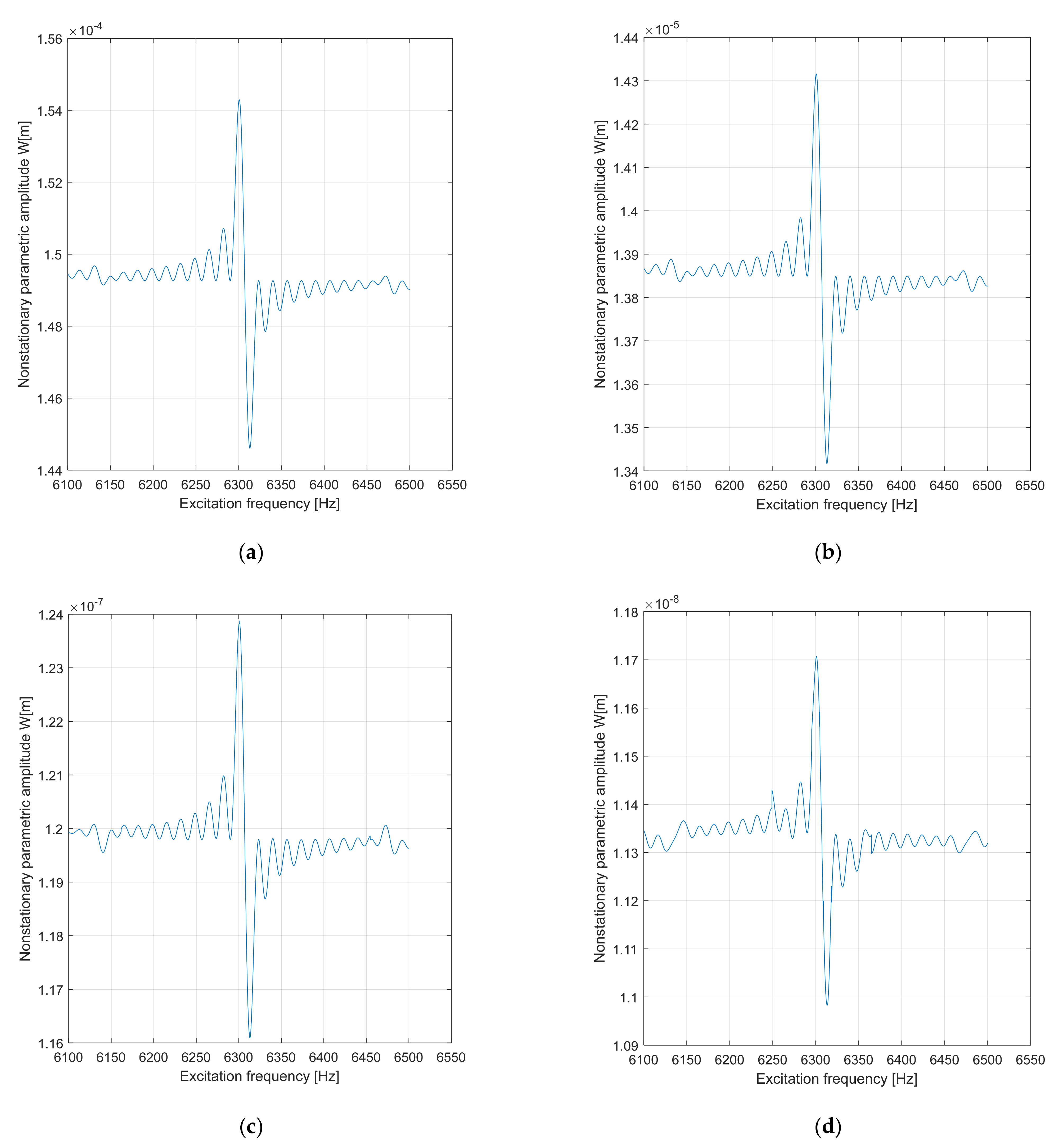
Figure 24 illustrates the nonstationary amplitude spectrum
of the FBVM for the bowl during the transition through the PPR region.
As for the tulip, a vast number of numerical tests was performed to arrive at a reasonable value for the sweep rate of the excitation frequency m = 1.4 × 10
−5 octaves/min. By analyzing the nonstationary parametric amplitude spectrum presented in
Figure 24 for
= (1.6–31.8) × 10
−3 and
= 0.10, the manifestation of beating effects as well as a significant decrease in the amplitude peaks with the increase in the damping ratio value in the range of (1.6–11.6) × 10
−3 can be found, while in the range of (11.6–31.8) × 10
−3, the decrease was more significant. The maximum peak of the amplitude was obtained when the excitation frequency was in close vicinity of the PPR for the bowl (6306 Hz). Each time the damping ratio increased at a rate of 0.01, the maximum peak amplitude decreased by more than 10 times (5 times for the tulip), because the bowl had a more considerable rigidity than the tulip.
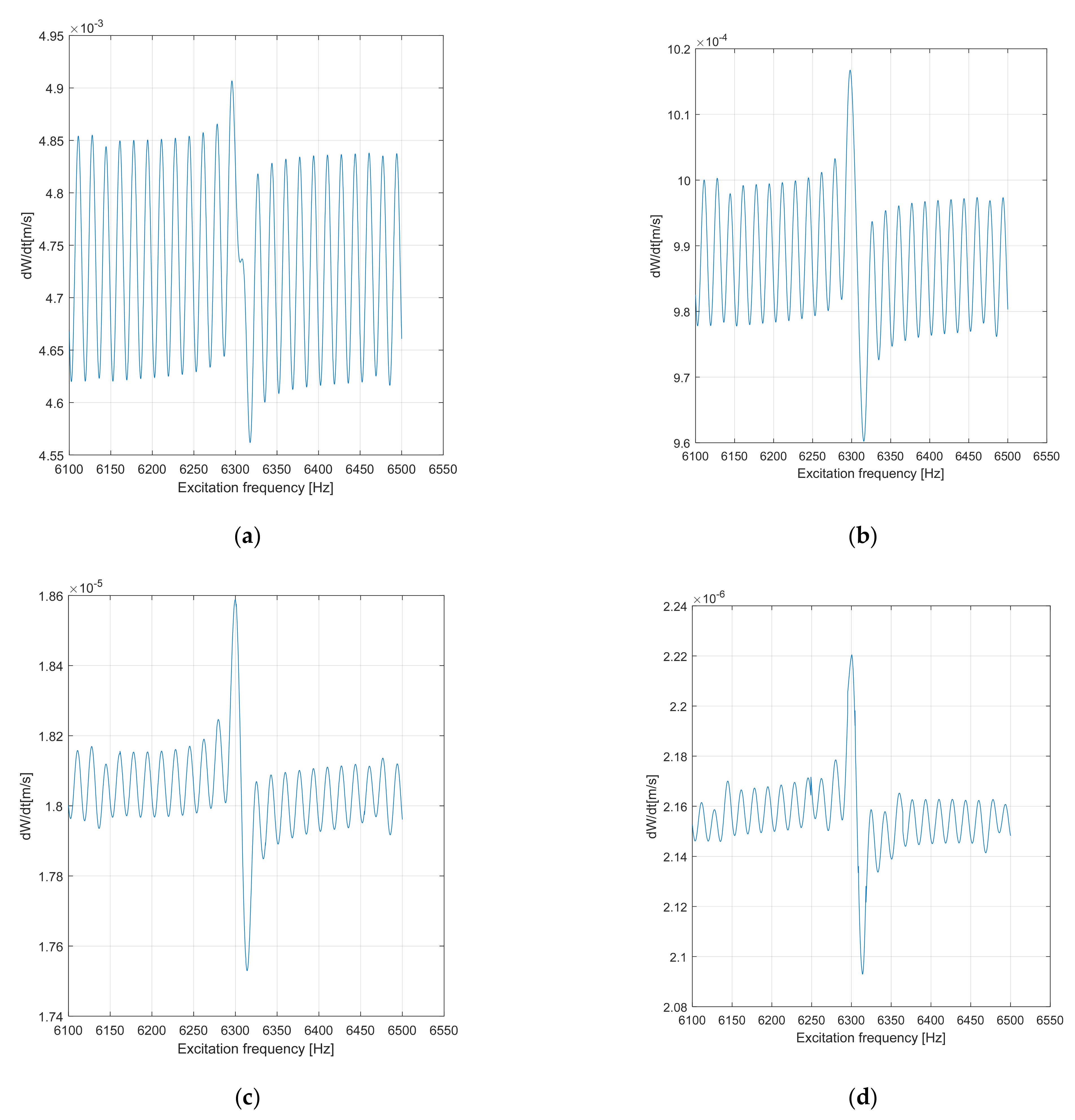
Figure 25 illustrates the nonstationary velocity amplitude spectrum
of the FBVM for the bowl during the transition through the PPR region.
When analyzing the graphs in
Figure 25, the moment of passing in close vicinity of the PPR was marked by a sudden increase in the peak of velocity amplitude, while the manifestation of beatings was like that of the nonstationary velocity amplitude spectrum for the tulip (see
Figure 22). The manifestation for the bowl was different than that for the tulip (see
Figure 22) because from the beginning, in the whole range of the damping ratio (0.0016–0.0318), the increase in the damping ratio had the effect of decreasing the maximum peak of the nonstationary velocity amplitude by approximately 5 times in the range of 0.0016–0.0116, while in the range of 0.0216–0.0318, the increase in the damping ratio had the effect of decreasing the maximum peak by more than 8 times. It can be concluded that the growth of the damping ratio had the beneficial impact of reducing the nonstationary velocity amplitude in the whole range (0.0016–0.0318) of the damping ratio.
Figure 26 illustrates the graphs of phase space
for the nonstationary FBVM of the bowl during the transition through the PPR region.
When analyzing the graphs in
Figure 26, the same manifestation for the bowl as for the tulip (see
Figure 23) can be seen, that being a transition to chaotic behavior for the FBVM of the bowl due to the presence of limit cycles or even strange attractors. However, this last conclusion needs to be certified by detailed analysis using the methods of chaotic movements. This manifestation is valid only in the damping ratio range of 0.0016–0.0096. One aspect that is evident is how the transition through the PPR region for the bowl was also an unstable one.
Unfortunately, there are no published studies which analyze in detail the dynamic behavior of each element of the AD for the FBVM (the tulip, bowl, and midshaft) apart from [
4], as all the studies analyzed the global dynamic behavior of the automotive driveshaft. As can be seen from this paragraph, the use of AMA coupled with Hamilton’s principle allowed the investigation of the stationary motion for the FBV movements of an AD’s tulip and bowl in the PPR region by computing the amplitude (see
Figure 10,
Figure 11,
Figure 14 and
Figure 15), the phase angle (see
Figure 7,
Figure 12,
Figure 13 and
Figure 16), and the dynamic instability frontiers (see
Figure 18 and
Figure 19) in the PPR region. In the meantime, the use of the AMA coupled with Hamilton’s principle allowed the investigation of the nonstationary motion for the FBV movements of an AD’s tulip and bowl in the transition through a PPR region by computing the amplitude spectrum (see
Figure 21 and
Figure 24), the velocity amplitude spectrum (see
Figure 22 and
Figure 25), and the velocity amplitude versus the amplitude in the phase space
(see
Figure 23 and
Figure 26).
Figure 23 and
Figure 26 allowed the investigation of the dynamic instability in the transition through the PPR region. As is noted in
Figure 21,
Figure 22,
Figure 23,
Figure 24,
Figure 25 and
Figure 26, the transition to the PPR region had an aspect of chaotic manifestation due to the manifestation of beating effects. To check whether this nonstationary dynamic behavior is deterministic chaos or a stochastic process, it would be necessary to use Lyapunov’s exponents method coupled with the Poincare map method. All these aspects represent novelties in the dynamic instability investigation for the AD. Based on the phenomena presented above, the direction for future research involves the study of chaotic motion generated by the FBVM of the AD elements. Another future research direction is to investigate the dynamic instability in the proximity of each possible resonance type for the stationary and nonstationary FBVM of the AD elements, such as subharmonic resonance, superharmonic resonance, and combination and internal resonance.


