Article

Combination of Transfer Learning Methods for Kidney Glomeruli Image Classification

Department of Computer Science and Information Engineering, National Quemoy University, Kinmen 89250, Taiwan
*
Author to whom correspondence should be addressed.
Appl. Sci. 2022, 12(3), 1040; https://doi.org/10.3390/app12031040
Submission received: 31 August 2021 / Revised: 15 January 2022 / Accepted: 17 January 2022 / Published: 20 January 2022
(This article belongs to the Special Issue Principles and Applications of Data Science)

Abstract

:
The rising global incidence of chronic kidney disease necessitates the development of image categorization of renal glomeruli. COVID-19 has been shown to enter the glomerulus, a tissue structure in the kidney. This study observes the differences between focal-segmental, normal and sclerotic renal glomerular tissue diseases. The splitting and combining of allied and multivariate models was accomplished utilizing a combined technique using existing models. In this study, model combinations are created by using a high-accuracy accuracy-based model to improve other models. This research exhibits excellent accuracy and consistent classification results on the ResNet101V2 combination using a mix of transfer learning methods, with the combined model on ResNet101V2 showing an accuracy of up to 97 percent with an F1-score of 0.97, compared to other models. However, this study discovered that the anticipated time required was higher than the model employed in general, which was mitigated by the usage of high-performance computing in this study.

1. Introduction

Acute kidney injury is a common and significant complication. And it has been proven that one of the factors that cause the disease to occur frequently is the increase in the widespread distribution of red blood cells and excessive inflammation. [1,2]. The pathophysiological mechanisms that explain the association between increased RDW scores and poorer prognosis remain unclear. According to current knowledge, an increase in RDW is the cause of microcirculation disorders. Older erythrocytes gradually lose the ability to damage cell membranes. This feature is especially important during the squeezing of nucleated cells through small diameter vessels in organs, such as the kidneys. The stiff and large erythrocytes observed in patients with high values of RDW could not enter through the capillaries and thus impaired blood flow through the microcirculation, leading to ischemia of the renal tissue [1].
Recently, kidney disease is increasingly being found in the spread of the coronavirus during the current pandemic [3]. The identification of the host of the second angiotensin-converting enzyme (ACE2) is the first step in the entry of viral infections into the body, where this host leads to cell fusion and entry into host cells in the lungs. Other epithelial cells, such as renal cells, have a high ACE2 expression [4]. As a result, several studies have shown that the long-term consequences of COVID-19 infection may cause COVID-19 patients to develop chronic kidney disease. The antigen capture technique showed that an increase in the SARS-CoV-2 protein in urine samples was detectable when compared to patients before the epidemic. By considering this condition, kidney disease detection needs some prerequisites to obtain the results quickly and accurately. Since COVID-19 is implicated in kidney function, this study aims in identifing how the anatomy of kidney disease is affected by COVID-19. Histopathology revealed that abnormalities in the kidney occur when the shape of the glomerulus in the kidney structure is different, eventually leading to chronic kidney disease [5]. Understanding how the complex structure of kidney tissue differs, requires the use of imaging technology to compare normal and diseased kidneys.
Until recently, there were two types of glomerular tissue disorders: sclerosed and focal-segmental sclerosed [6]. The difference between these two types may be seen in Bowman’s capsule structure around the glomerular network. Bowman’s visible capsule surrounds the glomerulus, suggesting that the glomerular tissue is undeniably normal, whereas Bowman’s capsule that seems faint or even disappears indicates that the glomerular tissue is unhealthy [7]. This explanation is supported by the morphological and Karpinski scores, which indicated the presence of a difference between nucleus and capillary lumens, and the number of areas (mesangial matrix) on the typical glomerular capillary lumens were absent. Moreover, the Bowman’s capsule was filled by collagen in glomerular non-healthy kidneys. Focal segmental sclerosis is a disease of the glomerulus that affects many people. A difference in glomerular size, the degree of leg process elimination and the alteration do the celial cells are all signs of this illness [6]. Figure 1 depicts the anatomy distinctions among three types of glomeruli. Imaging technology is predicted to aid in the accurate detection of individuals with renal disease, allowing for better medical performance. Furthermore, the model’s ability to analyze data will be determined by how much time is allotted to it. The transfer learning technique used in this study was taken from several machine learning models after reviewing various methods by considering the procedures and work results obtained. Bueno et al. [8] used UNet and SegNet to divide the glomerulus into three groups based on segmentation pixels. The data processing findings demonstrate that data prediction from the train data is accurate to 98.16 percent.
As a result, the combination of these approaches is used as a benchmark for comparing the proposed study with the EfficientNet method [9]. In the previous two years, this technique has been enhanced by altering the model’s structure, combining the models and employing the iterative model process. The ImageNet dataset, which comprises random pixel data (non-medical picture), has recently been used in some studies to show that this method’s accuracy rate approaches 99.70 percent [10]. This result is utilized as a proof-of-concept that the EfficientNet technique can provide high accuracy when utilizing the medical picture dataset. Therefore, the goal of this research is to demonstrate how this approach may be used in medical imaging collections.
The majority of deep learning in the categorization of glomeruli comprises of normal, sclerosed and non-glomerular classes, according to the prior studies. As a result, this study proposes three possible classifications: normal, sclerosed and focal-segmental sclerosed. Since focal-segmental sclerosed glomeruli [11] are a type of sclerosis that cause anomalies in the glomerular tissue and affect a large number of people, it is critical to correctly detect the focal-segmental anatomy of sclerosed glomeruli in kidney disease diagnosis.
The normal glomerulus, sclerosed glomerulus and focal-segmental glomerulus were all used to create this approach for transfer learning. Section 2 and Section 3 provide detailed explanations of the database, materials and research techniques, whereas Section 4 and Section 5 contain the results of the tests and conclusions.

2. Materials and Methods

This section details the procedures involved in conducting the study, including the data sources, methodologies and models used to enhance and manage the studies for improved outcomes.

2.1. Data and Preparation

The experimental data consisted of 5095 biomolecular pictures of the kidneys in png format, each of which was derived from 2926 photos of the segmentation data conducted by Bueno et al. [8,12]. These data can be used to benchmark the assessment data in a test classification system that divides the data into normal glomeruli and sclerosed glomeruli. Dimitris, in the Kaggle dataset [13], separated the 1584 pictures from the open data challenges, according to the form of the glomeruli tiles, into raw data and 585 additional focal-segmental images obtained from the study obtained by Kannan et al. [14].
The picture has a resolution of 256 × 256 pixels and is divided into three categories: normal, sclerosed, and focal-segmental. This clustering was performed to show the part of the experimental section’s categorization findings that were correct. Rosenberg et al. [6] conducted studies on focal-segmental sclerosis. Martin-Navarro [11] discovered focal-segmental kidney disease types in pulmonary sarcoidosis, while Asinobi et al. [15] performed histology on the trend of children’s nephrotic syndrome in Ibadan, Nigeria. Since the research into the identification of focal-segmental sclerosis has presented few findings, it is necessary to conduct preprocessing on the image dataset by rotating, changing picture size and replicating images to achieve uniformity. Since the data train is more accurate, this technique is suited for the testing the focal-segmental class. As a result, the information gathered is split into three categories.
Data preparation was performed using previously acquired data, according to the most recent data source. In this step, the transfer learning approach requires data labeling on the dataset to identify the different classes. The HuBMAP dataset was used to label the data train encoded into the path annotation, where the primary data was an image file in the Big TIFF format that was then examined on the raw tiles using Python programming. The Mendeley dataset consisted of 31 SVS pictures that were provided as raw data and converted to PNG files. Data labeling was created for focal-segmental sclerosed, and the data was separated into train, test and validation. Given the variety of techniques used, we considered executing the code offline using the system specified in Table 1 (which was compatible with the Python version) to conduct all tests, as well as performing the experiments using the cloud service using GPU instances.
The script code was obtained from past research and experiments, and its structure and methods were modified to meet our study goals. The goal of the project was to assess the performance of the experiments and compare them to the dataset that was chosen. As a result, the purpose of this research was to test and enhance the accuracy of picture categorization using the existing image dataset.

2.2. Exploration Data Analysis

The presence or absence of the ring was determined by assessing the circular shape of Bowman’s capsule in the nucleus of the glomerular cells. We used the breadth of the red blood cell distribution (RSVP) to distinguish between sclerosed and localized segmental illness, in addition to the study’s main emphasis. In the training data portion, this picture recognition method is examined first.
The utilized dataset, as indicated in the preceding section, is an unlabeled dataset collected from three sources. It was then separated into two halves for use as training and test sets. Additionally, one component created a validation set to demonstrate the viability of training or testing according to a predefined categorization. As a result, this study developed a normal, sclerosed and focused training, test and validation set. Figure 2 depicts the validation set data, which includes the true label for each class presented.
With a scale of 3:3:1, the data set was split into the train, test and validation sets. The train set had 2100 photos, with 700 pictures for each class, 2290 test sets with 763 pictures for each class and 705 pictures validation set with 235 pictures for each class. Figure 3 depicts the findings, which include a graph of each created set. The training set and validation set as the pre-trained models in the transfer learning process, are generalized based on the dataset’s objectives.
The dataset utilized must be ignored since the data is generalized; therefore, the image is shrunk into 150 × 150 pixels before the data training process. This step has an influence on the resolution of the loaded image, so make sure it meets the criteria for intensity. The count number ranges from 0 to 8000, and the beginning pixel value is on a scale from 0 to 1. Figure 4 depicts an example of the picture data that meets the learning process’s criteria. The example image does not reflect all image intensity values from the dataset, but it does confirm that the data imported is correct.

2.3. Efficient Network (EfficientNet)

Since it has fewer work parameters to optimize the time resources needed, the EfficientNet design necessitates considerable relevance in data processing performance [9]. EfficientNet is comparable to the MobileNetV3 model [16], which uses the MBConv mobile inverted bottleneck as the fundamental building component of its design. The squeeze-excitation layer in the process [17], separates this model from prior versions. Before the picture is extracted further, Figure 5 reveals its resemblance to the previously generated layers and combined additional model to the last layer for obtaining improved results. The schema of the proposed combination model takes the form of a dense layer, in which it is possible to have more of the model than the bundle layer. Afterwards, the design was created after the transfer learning process on each model was completed, since this combination needs the first trained model to process the whole model in one design. However, because this layering issue was still extremely parametric, the impact resulted in a decreased efficiency. Furthermore, as compared to the conventional layers, the combination with depth-wise separated convolution reduces computation by a factor of k2. When the method was presented, the difference was obvious owing to a mix of compound scaling between the scaling width, depth and resolution, with the aim of improving the overall performance using the available resources.
Compound scaling has two stages: finding the scalping dimension parameters of the baseline network on the resource input using a grid search, and applying the coefficients obtained from adjusting the input dimensions on the baseline network to influence the size of the target model or computational budget, using the coefficients obtained from adjusting the input dimensions on the baseline network. Tan et al. [9] found a mathematical equation that employs the compound coefficient to equalize the scale throughout the network breadth, depth and resolution, as shown below:
depth : d = α ϕ
width : w = β ϕ
resolution : = γ ϕ
s . t . α · β 2 · γ 2 2
α 1 , β 1 , γ 1  
where the variables α , β , γ are the constants obtained from a small grid search. Logically, ϕ is a user-controlled coefficient regarding the number of resources available in model scaling, where α , β , γ determine the additional resources at the network width, depth and resolution, respectively. In particular, the floating-point operations per second (FLOPS) of the convolution process was proportional to the variables d , w 2 , r 2 by doubling the network depth, even though the network width and resolution increased four times. Scaling ConvNet will increase FLOPS by a total of ( α β 2 γ 2 ) ϕ because convolution operations usually dominate the computeing costs presented on ConvNet. EfficientNet contains the same architectural components as the convolutional network in general, despite its distinct working technique.
The EfficientNet-B7 [18] and EfficientNet-L2 [19] models from the EfficientNet architecture are used in this research. These two models are EfficientNet’s final models, which have a higher level of precision and scalability than previous EfficientNet models.

2.4. Residual Network (ResNet)

We picked the ResNet model as one of the models in this experiment, as a contrast to the approach we evaluated. ResNet, being the most widely used technique, requires layers to be reformulated as learning residual functions that refer to the layer inputs rather than the learning non-referenced functions [20]. ResNet has an advantage over other models, in that it does not add many layers to directly match the underlying mapping. In one of the examples, ResNet piled the leftover blocks at the top of each network form, illustrating the transfer of the layer work to the next processed layer in ResNet-50, which has 50 layers.
Formally, the function that represents how ResNet works is ( x )   = ( x ) x , where ( x ) is underlying mapping. The original mapping was recast into ( x ) + x . There is empirical evidence that these networks are easy to manipulate and optimize, and can gain accuracy by considering the addition of depth to the network without creating new layers.
This research uses the ResNet101V2 and ResNet50V2 models. The equation for this model is to utilize 50 remaining blocks so that the learning process does not take as long to estimate. The only difference between these two models is how the mappings are identified in the learning process [21]. ResNetV2 has this capacity by evaluating the form of the mapping before stacking the rest of the blocks. To put it another way, the model architecture changes as a result of the process. Constant scaling, exclusive gating and shortcuts, such as convolutional or dropout shortcuts, are available in some situations. As a result, while performing the tests, this difference had a substantial impact.

2.5. Very Deep Convolutional Networks for Large-Scale Image Recognition (VGG)

Furthermore, we chose the VGG model as a comparison model in this study, based on the numerous studies that used it in recent years. VGG [22] is a common picture classification method. The VGG’s architecture adds depth to the network layer by using a modest network width. The network employs tiny 3 × 3 filters, where the layer components are made out of the same three blocks, as is standard on CNN. A network, on the other hand, is defined by its simplicity and is otherwise organized with additional components, such as pooling layers and completely linked layers [23]. The VGG16 and VGG19 models were used in this VGG approach.
These two models are the VGG method’s final models, with a higher readout rate for the image processing than the other models. VGG16 has 16 weight layers, each of which consists of 13 3 × 3 convolutional layers and 3 fully connected layers, whereas VGG19 has 19 weight layers, each of which consists of 16 3 × 3 convolutional layers and 3 fully connected layers. The VGG19 model differs in that it adds a 3 × 3 convolutional layer to each max pool block with varying sizes, depending on the max pool block.
When compared to numerous newer techniques, the VGG method’s performance is deemed steady. This outcome was demonstrated by the method’s adaptability, which allowed new methods to be created [8]. The simplicity of the VGG approach influenced other methods that could enhance analytical findings without entirely altering the existing architecture.

3. Results

3.1. Independent Model Experiment Results

We used several treatments for each model in a transfer learning procedure. When presented with the same treatment, the differing model designs caused problems in the learning process. The study began with a comparison of two identical models in the same architecture, with the historical correctness of the models being assessed (Table 2)
VGG19. VGG19 was tested by training a 3 × 3 convolutional layer using an ImageNet classification model using average pooling. The output was assessed by permitting numerous fine-tuning approaches, such as the activation of the rectified linear unit (ReLU) dense layer to achieve a low learning rate, the activation of the soft-max layer and saving checkpoints on the best model [24]. The period began with an evaluation of the time spent during training, the number of total parameters processed and the storage of a learning process evaluation. With a total parameter of 20,090,435, VGG19 successfully completed the training with an average model accuracy of 0.9361, validated with a high value of 0.9390 and the maximum accuracy value of 0.9981. It is possible to infer that the two VGG models can depict models that are good enough to be classed as medical pictures, based on the findings of the two models. The accuracy of the case suggested by the VGG model was in the range of 0.80 to 0.90 and above. In terms of the value scale, the VGG19 value is an appropriate category to use as an image classification model, as shown in Table 3. 
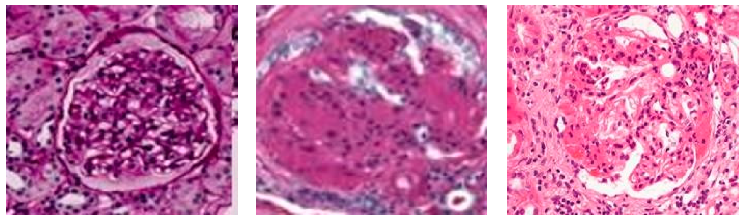
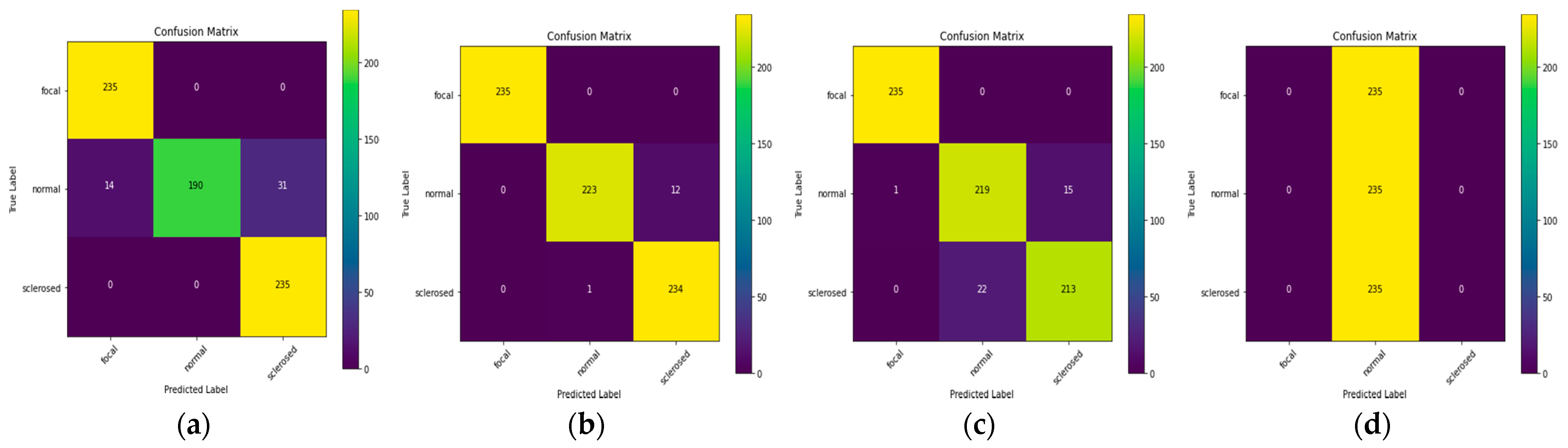
Figure 6a demonstrates that the original value’s correlation with the predicted value shows a high color prediction for the focal and sclerosed classes, while the projected normal class has a sufficient color in the classification.
ResNet101V2. The architectural resemblance between these two models may also result in the same model performance configuration. On the convolutional network, both model sets are constructed with a resolution of 150 × 150 using ImageNet weight. With a logistic regression (LR) value of 0.01 and a momentum value of 0.7, both of these models employed stochastic gradient descent (SGD) optimization for fine-tuning [25]. This setting is an iterative approach for fine-tuning the objective function. Each high-accuracy validation point was saved in the model checkpoint function and utilized as a weight model in a pre-trained model.
ResNet101V2 runs 55,637,123 parameters in total. After determining these parameters, ResNet101V2 completed the training with an average accuracy of 0.9815, which was confirmed by the maximum value of 0.9801, for which the greatest accuracy score was 1000. The training results, as shown in Table 3, demonstrate that each model employed in the experiment had the best accuracy.
EfficientNetB7 and EfficientNetL2. The EfficientNet model employed in this study differs significantly from the previous one. EfficientNet-B7 can operate using ImageNet weight, but EfficientNet-L2 requires noisy student weight as a pre-trained model, according to prior research. This occurred because EfficientNet-L2 was incompatible with the ImageNet weights, when the number of layer weight initiations of the model differed. The unevenness of the pre-trained models employed was caused by weight fluctuations, although this is an exception to correctly performing the training process. Even when running on different models, these two models employed the same fine-tuning. The average-pool layer was added to the end of the flattened layer. In addition, the use of the ReLU feature and a dropout layer with a value of 0.2 created a dense layer. A thick layer was seen in the last portion. Furthermore, this approach employed an optimizer in the form of Adam [26], throughout the compilation process.
With a training parameter of 2,625,539, EfficientNet-B7 achieved an average accuracy of 0.9461. The highest value, 0.9291, was used to confirm this accuracy, and the maximum accuracy was 0.9662. Meanwhile, EfficientNet-L2 utilized a training parameter of 5,640,195, with an average accuracy of 0.3333 as a consequence. The greatest accuracy as 0.3424, and this accuracy was confirmed using the highest value of 0.3333.
The EfficientNet-B7 and EfficientNet-L2 designs had significant variations in their training outcomes. EfficientNet-B7 does a far better job at presenting results than EfficientNet-L2. Figure 6c,d indicate that the EfficientNet-L2 predictions show that everything is in the usual class, but the EfficientNet-B7 predictions are evenly distributed in each class. These findings demonstrate that the allied model does not generate accurate transfer learning predictions.
Based on the training data, we may infer that the EfficientNet model does not have a high level of accuracy. The inequality found in the EfficientNet-L2 model indicates that the accuracy findings in EfficientNetB7 are inconsistent. The model’s incompatibility with the dataset utilized, on the other hand, prevents it from producing the optimal results.

3.2. Combining Model Experiment Results

After reviewing the results of the experiment, we tried again, this time using many models that were judged unfit for classification. As shown in Table 3, the findings of Effi-cientNet-L2 do not exhibit a high degree of accuracy, especially when compared to the criteria set by the trials. In a model with low accuracy, a high yield model has a substantial impact on improving accuracy. The experiments on a cognate or unrelated model confirmed this idea.
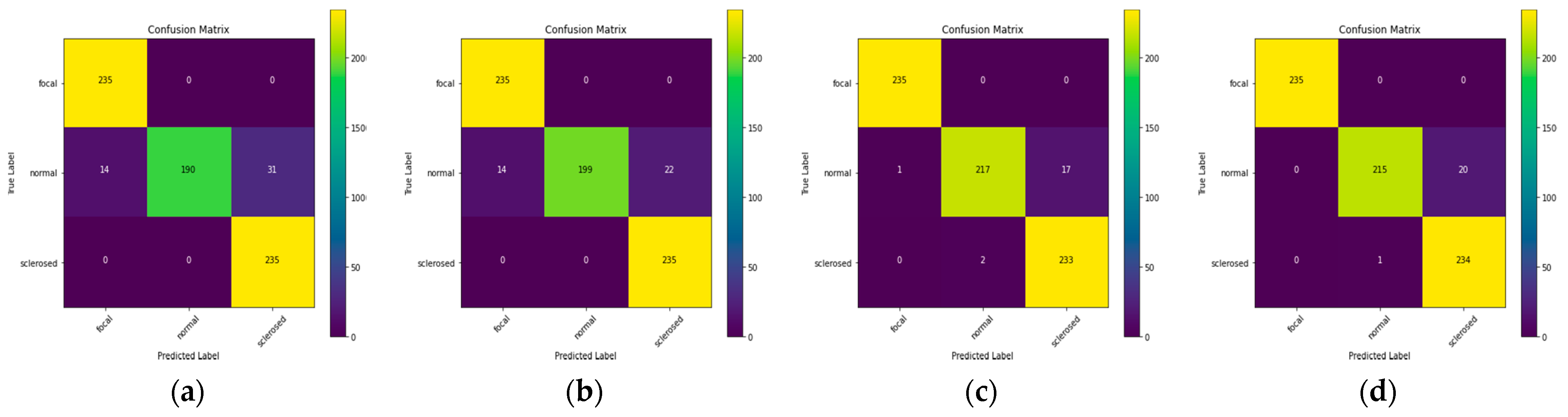
Combination Allied Model. The accuracy value obtained from the combination of the associated models is dependent on the base model utilized. The value obtained in the combination model was proportional to the model’s independent accuracy value. This experiment was carried out on three family models that is VGG, ResNet, and EfficientNet, all of which have different layer designs despite being related. With VGG16 as the basic model, the VGG model accuracy is 93.62 percent, as shown in Table 4. According to Figure 7, the normal class distribution offers less predictive data than the focused and sclerosed classes.
Combination Cross-Model. Cross-model combination refers to the model that is prioritized in order to enhance its accuracy value, limiting the models that may be combined to those that meet these requirements. EfficientNet-L2 and ResNet 101, for example, confirmed the need to improve. As a result, it is necessary to properly test each of these two models.
According to the base model employed in these tests, there are some varied categorization findings. Table 4 indicates that the classification results of Res-Net101V2 may enhance the accuracy results of EfficientNet-L2 by approaching the ResNet101V2 value independently, by achieving 97.16 percent. The projected value in Figure 7c is affected by this finding, with the distributions of each class matching the original value with a few erroneous values.
Combination Multivariate Model. EfficientNet-L2 has risen by up to two times while using ResNet101 as the basic model, compared to the prior trial when the model was conducting independent training. In this situation, ResNet101 has a low accuracy value, but it is still better than EfficientNet-L2; thus, the gain is not substantial. As a result of attempting to add another model with greater accuracy to this combination, two VGG models are used in the classification process as a multi-model combination experiment. The accuracy value from the combination model produces similar results, which are better than the EfficientNet-B7 model independently.
VGG, ResNet and EfficientNet were all used to perform model tests. One model from each model family was selected as the basic model, since it generated high accuracy results. Each model’s accuracy has greatly improved as a result of this setup. This model’s combination experiment takes two to three times as long as the models that conduct experiments individually, depending on the number of models that can be combined. As shown in Table 4, the time necessary to combine three particular models to obtain the best results, is equal to the training time for each model. This impact does not apply to the combinations inside the same model, since the predicted outcomes do not need numerous iterations, allowing the results to be taken from the same model without having to retrain the model. However, by combining the two models in the same model, it does not significantly enhance the model classification accuracy. As a result, in order to obtain more optimum findings, the time efficiency of this model combination experiment must be addressed.

3.3. Evaluation

We compared and contrasted two categorization studies, each of which had its own set of benefits and drawbacks. This study discovered mixed findings from all of the models evaluated in the different model trials. These outcomes were influenced by the model architecture used, as well as the fine-tuning the model. The projected time for each model was also dependent on the parameters that were utilized during training; the more parameters that are used, the longer the training will take. Furthermore, the training per epoch method produced diverse graphs. The graphs observed did not develope steadily and there was significant irregularity in the graphs acquired. As a result, it is not recommended to use a model with such dramatic findings for classifying medical pictures. The F1-score evaluation parameter was utilized to examine the value of each class and the mean of each model. The accuracy and recall levels in the arithmetic theorem provided this F1-score. Table 5 indicates that the normal glomeruli class dominates the EfficientNet-L2 model’s prediction results, which is consistent with Figure 6d, which displays predictions in the normal class. In Table 6, the class predictions for ResNet101V2 are dispersed in each class with a modest error rate, as shown in Figure 6b, in which the original and predicted values overlap fairly well.
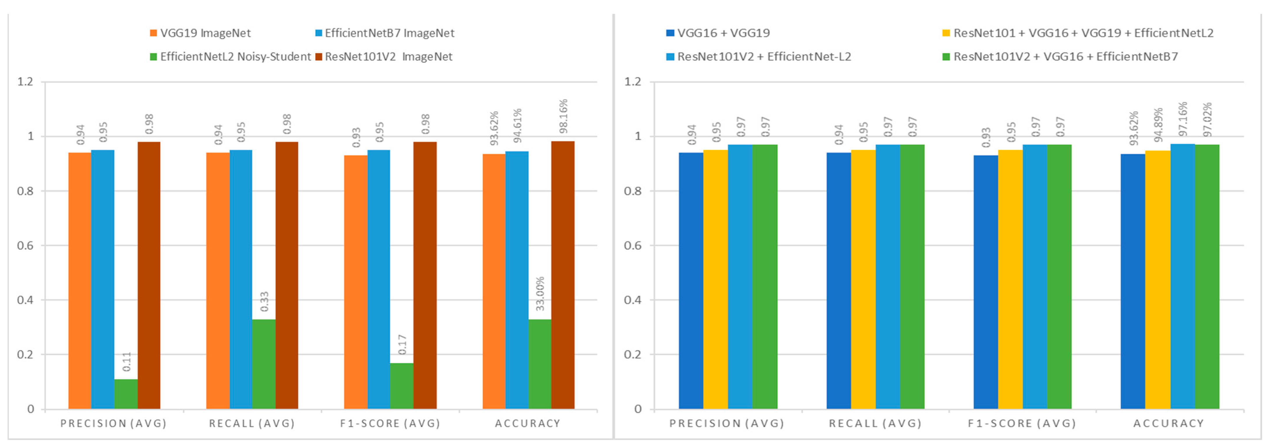
When comparing the independent assessment models displayed in Figure 8 (left), it is clear that EfficientNet-L2 is not acceptable as a reference model for medical image classification since it has the lowest evaluation value, with just a 0.17 F1-score. With an F1-score of 0.98, ResNet101V2 is the best reference model for medical picture categorization. The findings of the combination technique experiment were identical for each model combination. Table 4 demonstrates that the model combination experiment yields findings that are more than 90% accurate over time. Figure 8 shows this outcome, with a predictive value in each class’s distribution that matches the original value and many error values in the incorrect predictions.
Based on these findings, this study assesses each model’s classification prediction class to demonstrate the impact of accuracy on model performance. The three model combination trials revealed a metric assessment value that was relatively steady with a low error rate (Table 7, Table 8 and Table 9). The prediction value of the class distribution, which is near to 1.00, indicates that the forecast value closely follows the actual value. Figure 8 (right) indicates that all the combination technique trials achieved an assessment value of more than 0.90, with an average F1-score of 0.955. However, the predicted training time for this model combination experiment was very high, with an average of 28 min required, making it less time efficient.

4. Discussion

Based on the research results, the combination of deep transfer learning methods to classify kidney disease in glomeruli has many characteristics, in terms of technical data collection, exploratory data analysis and also the comparison with relevant research. By prioritizing the data obtained from previous research coupled with the latest data from relevant health institutions, we attempted to filter the data that was suitable and with a high degree of similarity, so that the data collected could improve the results of machine learning. This technique was also carried out in previous research, by Manzo et al. [29], which used CX-ray images data from various sources to detect COVID-19 disease through machine learning. However, the approach of this study used segmentation techniques from diseases images; therefore, its steps are quite tedious. Meanwhile, we used the diseased kidney data as a dataset to be studied by the machine. As a result, when testing the data, the machine already recognized the exact criteria for the diseased kidney.
For our data exploration, we focused on determining the level of the distribution of red blood cells (RSVP) that appeared in the diseased kidney image by adjusting the pixels and brightness of the image, so that it appeared more proportional. This technique is in line with the method used by Pavinkurve et al. [30], which performs image preprocessing to detect the same disease. In this study, this technique was able to overcome the problem of image bias in CT scan images. The suitability of this technique with the results of the CT scan images is considered as being capable of facilitating the machine learning process to obtain the object of the image. On the other hand, this study utilizes subject matter that is often studied in previous studies, but is unique in its application of the methods.
This research, which focuses on discussing kidney disease, has relevant developments with the same objectives, including the utilization of image classification that applies different machine learning methods in various amounts, and the segmentation of images by combining classification and segmentation methods. We obtained this perspective by developing a combined model research method that utilized various types of methods to compare which results were more accurate and precise, as was also performed by Bueno et al. in two kidney disease studies, which combined the resulting segmentation method with the adopted classification method to find the significant differences in diseased kidneys. Furthermore, they found a new method to produce a more accurate optimal image classification method for diseased kidneys. By utilizing the results obtained in the research of Bruno et al., we expanded the research by adding various transfer learning methods that had been previously studied and adding to the dataset used, so that the results obtained were compared with each other to achieve a higher accuracy value.
The technique that we found in this study is also supported by previous research, which uses a variety of techniques. The use of automatic learning in kidney disease is our focus for the development of the current research. This is in line with what was conducted by Altini et al. [7], who developed research on kidney disease using the DeepLab method through MATLAB, whereby the learning process can present the detailed results requested by the user to facilitate comprehensive research performance. Meanwhile, several previous studies used neural network techniques, either by directly using the model or installing a new model. This technique was found in a study developed by Barros et al. [27] and Marsh et al. [28], by installing neural networks to find the types of glomerular proliferative kidney disease, which implements neural networks in the form of a full model to detect the type of tubulointerstitial kidney glomeruli disease. This condition prompted us to conduct research on a combination of models that utilize neural networks in the transfer learning model. Thus, we could develop our research based on the learning scheme of neural networks in each of the models we used. In addition, the research we used was also supported by the research of Kannan et al. [14], who researched the differences in the sclerosed shape of diseased kidney glomeruli using the CNN model in the form of Inception V3.

5. Conclusions

To obtain the desired results, medical image categorization necessitates the following procedures. The fundamental task in deep machine learning is to find an appropriate model to run on a medical imaging dataset, which may be accomplished by altering an existing model, developing a new model or applying an existing model. This study compared each model to obtain a high classification accuracy value by using an existing model on a medical picture dataset. This study integrated many models into a single model to obtain a higher and more consistent classification accuracy value from the current models.
We found the EfficientNet model to be weak in comparison to various other machine learning models after analyzing the suggested technique. This study demonstrated that EfficientNet-L2 is not yet ideal for correctly identifying medical pictures, since it only achieves a 33 percent accuracy rate. As a result, the EfficientNet model is ineffective in classifying medical images independently. However, we discovered that the ResNet model is a good fit for categorizing medical images. We discovered a ResNet101V2 that is appropriate for usage in the medical picture dataset gathered during the application of current models. ResNet101V2 has the best accuracy of all the tests performed on an independent model, with values over 98.16 percent. As a result of this finding, it is clear that certain models are less accurate than others, necessitating the use of alternative techniques. As a result, combining models becomes a new experiment in order to improve the accuracy of the unfavorable model.
The allied, cross and multivariate models were evaluated in this combination experiment. The classification results from the three trials demonstrate that by using the best model as the base model, all combination models attain accuracy values above 90%. This application focuses on the best model in order to enhance the less-than-ideal model. Since it works highly depending on the number of merged models, the combined model has flaws in terms of the computation time. However, when compared to the models created separately, the absolute accuracy of the combined model is the highest.
With the advancement of medical image classification research, it is important to address the various aspects that influence the model employed. Existing models may be improved by inputting or altering various optimization variables to obtain the best results for the combined model, as well as the procedures required to streamline the model process’s estimated time and its impact on the model architecture. To put it another way, this research is anticipated to continue discovering the best outcomes in terms of architecture and the predicted time necessary, so that the accuracy value attained is achieved using the best methods and models.

Author Contributions

Conceptualization, H.-C.L. and A.F.A.; methodology, H.-C.L.; software, A.F.A.; validation, H.-C.L. and A.F.A.; formal analysis, H.-C.L.; investigation, A.F.A.; resources, A.F.A.; data curation, A.F.A.; writing—original draft preparation, A.F.A.; writing—review and editing, H.-C.L.; visualization, A.F.A.; supervision, H.-C.L.; project administration, H.-C.L.; funding acquisition, H.-C.L. All authors have read and agreed to the published version of the manuscript.

Funding

This research was funded partially by the Ministry of Education of Taiwan (R.O.C.) via the Artificial Intelligence Talent Cultivation Project and was supported partially by the Ministry of Science and Technology of Taiwan (R.O.C) through National Center for High-performance Computing.

Institutional Review Board Statement

Not applicable.

Informed Consent Statement

Not applicable.

Data Availability Statement

Not applicable.

Acknowledgments

We thank Khrisna Kumar S for their input in the project. This program code is modified from Kaggle to suit the needs of the dataset and the architecture used. This research is based on an image database supported by the Cancer Imaging Archive. This work makes use of the supercomputing facilities managed by the Artificial Intelligence Laboratory, National Quemoy University and the online facilities from Ministry Science and Technology of Taiwan through Taiwan Cloud Computing Preferences. This research thanks Google for providing a valuable source of data for our research.

Conflicts of Interest

The authors declare no conflict of interest.

References

  1. Duchnowski, P.; Hryniewiecki, T.; Kuśmierczyk, M.; Szymański, P. The usefulness of selected biomarkers in patients with valve disease. Biomarkers Med. 2018, 12, 1341–1346. [Google Scholar] [CrossRef] [PubMed] [Green Version]
  2. Duchnowski, P.; Hryniewiecki, T.; Kuśmierczyk, M.; Szymański, P. Anisocytosis predicts postoperative renal replacement therapy in patients undergoing heart valve surgery. Cardiol. J. 2020, 27, 362–367. [Google Scholar] [CrossRef] [PubMed] [Green Version]
  3. George, S.; Pal, A.C.; Gagnon, J.; Timalsina, S.; Singh, P.; Vydyam, P.; Munshi, M.; Chiu, J.E.; Renard, I.; Harden, C.A.; et al. Evidence for SARS-CoV-2 spike protein in the urine of COVID-19 patients. Kidney 2021, 2, 924–936. [Google Scholar] [CrossRef]
  4. Kaur, S.P.; Gupta, V. COVID-19 Vaccine: A comprehensive status report. Virus Res. 2020, 288, 198114. [Google Scholar] [CrossRef] [PubMed]
  5. Kolhe, N.V.; Fluck, R.J.; Selby, N.M.; Taal, M.W. Acute kidney injury associated with COVID-19: A retrospective cohort study. PLoS Med. 2020, 17, e1003406. [Google Scholar] [CrossRef] [PubMed]
  6. Rosenberg, A.; Kopp, J. Focal segmental glomerulosclerosis. Clin. J. Am. Soc. Nephrol. 2017, 12, 502–517. [Google Scholar] [CrossRef] [PubMed] [Green Version]
  7. Altini, N.; Cascarano, G.D.; Brunetti, A.; Marino, F.; Rocchetti, M.T.; Matino, S.; Venere, U.; Rossini, M.; Pesce, F.; Gesualdo, L.; et al. Semantic segmentation framework for glomeruli detection and classification in kidney histological sections. Electronics 2020, 9, 503. [Google Scholar] [CrossRef] [Green Version]
  8. Bueno, G.; Fernandez-Carrobles, M.M.; Gonzalez-Lopez, L.; Deniz, O. Glomerulosclerosis identification in whole slide images using semantic segmentation. Comput. Methods Programs Biomed. 2020, 184, 105273. [Google Scholar] [CrossRef] [PubMed]
  9. Tan, M.; Le, Q.V. Efficientnet: Rethinking model scaling for convolutional neural networks. In Proceedings of the 36th International Conference on Machine Learning ICML, Jacksonville Beach, FL, USA, 11 June 2019; pp. 10691–10700. [Google Scholar]
  10. Foret, P.; Kleiner, A.; Mobahi, H.; Neyshabur, B. Sharpness-aware minimization for efficiently improving generalization. arXiv 2020, arXiv:2010.01412. [Google Scholar]
  11. Martín-Navarro, J.A.; Gutiérrez-Sánchez, M.J.; Petkov-Stoyanov, V.; Justo-Ávila, P.; Ionela-Stanescu, R. Glomerulonefritis focal y segmentaria en paciente con sarcoidosis pulmonar. Nefrol 2013, 33, 431–433. [Google Scholar]
  12. Bueno, G.; Gonzalez-Lopez, L.; Garcia-Rojo, M.; Laurinavicius, A.; Deniz, O. Data for glomeruli characterization in histopathological images. Data Brief 2020, 29, 105314. [Google Scholar] [CrossRef] [PubMed]
  13. Dimitris. HuBMAP: Glomeruli Tiles and Mosaics, Kaggle. 2020. Available online: https://www.kaggle.com/anadelta/hubmap-glomeruli-tiles (accessed on 17 March 2021).
  14. Kannan, S.; Morgan, L.A.; Liang, B.; Cheung, M.G.; Lin, C.Q.; Mun, D.; Nader, R.G.; Belghasem, M.E.; Henderson, J.M.; Francis, J.M.; et al. Segmentation of glomeruli within trichrome images using deep learning. Kidney Int. Rep. 2019, 4, 955–962. [Google Scholar] [CrossRef] [PubMed] [Green Version]
  15. Asinobi, A.O.; Ademola, A.D.; Okolo, C.A.; Yaria, J.O. Trends in the histopathology of childhood nephrotic syndrome in Ibadan Nigeria: Preponderance of idiopathic focal segmental glomerulosclerosis. BMC Nephrol. 2015, 16, 213. [Google Scholar] [CrossRef] [PubMed]
  16. Howard, A.; Sandler, M.; Chen, B.; Wang, W.; Chen, L.-C.; Tan, M.; Chu, G.; Vasudevan, V.; Zhu, Y.; Pang, R.; et al. Searching for MobileNetV3. In Proceedings of the International Conference on Computer Vision, Seoul, Korea, 27 October–2 November 2019; pp. 1314–1324. [Google Scholar] [CrossRef]
  17. Hu, J.; Shen, L.; Albanie, S.; Sun, G.; Wu, E. Squeeze-and-excitation networks. IEEE Trans. Pattern Anal. Mach. Intell. 2020, 42, 2011–2023. [Google Scholar] [CrossRef] [PubMed] [Green Version]
  18. Xie, Q.; Luong, M.-T.; Hovy, E.; Le, Q.V. Self-training with noisy student improves imagenet classification. In Proceedings of the 2020 IEEE/CVF Conference on Computer Vision and Pattern Recognition (CVPR), Seattle, WA, USA, 13–19 June 2020; pp. 10684–10695. [Google Scholar]
  19. Pham, H.; Dai, Z.; Xie, Q.; Le, Q.V. Meta pseudo labels. arXiv 2020, arXiv:2003.10580. [Google Scholar]
  20. He, K.; Zhang, X.; Ren, S.; Sun, J. Deep residual learning for image recognition. In Proceedings of the 2016 IEEE Conference on Computer Vision and Pattern Recognition (CVPR), Las Vegas, NV, USA, 27–30 June 2016; pp. 770–778. [Google Scholar] [CrossRef] [Green Version]
  21. He, K.; Zhang, X.; Ren, S.; Sun, J. Identity mappings in deep residual networks. In Computer Vision—European Conference on Computer Vision; Springer: Cham, Switzerland, 2016; pp. 630–645. Available online: https://link.springer.com/chapter/10.1007/978-3-319-46493-0_38 (accessed on 23 February 2021).
  22. Zhu, J.; Shen, B.; Abbasi, A.; Hoshmand-Kochi, M.; Li, H.; Duong, T.Q. Deep transfer learning artificial intelligence accurately stages COVID-19 lung disease severity on portable chest radiographs. PLoS ONE 2020, 15, e0236621. [Google Scholar] [CrossRef] [PubMed]
  23. Simonyan, K.; Zisserman, A. Very deep convolutional networks for large-scale image recognition. In Proceedings of the 3rd International Conference on Learning Representations, ICLR 2015, San Diego, CA, USA, 7–9 May 2015; pp. 1–14. [Google Scholar]
  24. Javid, A.M.; Das, S.; Skoglund, M.; Chatterjee, S. A ReLU dense layer to improve the performance of neural networks. In Proceedings of the ICASSP 2021–2021 IEEE International Conference on Acoustics, Speech and Signal Processing (ICASSP), Toronto, ON, Canada, 6–11 June 2021; pp. 2810–2814. Available online: http://arxiv.org/abs/2010.13572 (accessed on 3 March 2021).
  25. Sra, S.; Nowozin, S.; Wright, S.J. Optimization for Machine Learning; MIT Press: Cambridge, MA, USA, 2012. [Google Scholar]
  26. Kingma, D.P.; Ba, J. Adam: A method for stochastic optimization. In Proceedings of the 3rd International Conference on Learning Representations, ICLR 2015, San Diego, CA, USA, 7–9 May 2015; Available online: https://arxiv.org/abs/1412.6980#:~:text=WeintroduceAdam%2C (accessed on 4 February 2021).
  27. Barros, G.O.; Navarro, B.; Duarte, A.; Dos-Santos, W.L.C. PathoSpotter-K: A computational tool for the automatic identification of glomerular lesions in histological images of kidneys. Sci. Rep. 2017, 7, srep46769. [Google Scholar] [CrossRef] [PubMed] [Green Version]
  28. Marsh, J.N.; Matlock, M.K.; Kudose, S.; Liu, T.-C.; Stappenbeck, T.S.; Gaut, J.P.; Swamidass, S.J. Deep learning global glomerulosclerosis in transplant kidney frozen sections. IEEE Trans. Med Imaging 2018, 37, 2718–2728. [Google Scholar] [CrossRef] [PubMed]
  29. Manzo, M.; Pellino, S. Fighting together against the pandemic: Learning multiple models on tomography images for COVID-19 diagnosis. AI 2021, 2, 261–273. [Google Scholar] [CrossRef]
  30. Pavinkurve, N.P.; Natarajan, K.; Perotte, A.J. Deep vision: Learning to identify renal disease with neural networks. Kidney Int. Rep. 2019, 4, 914–916. [Google Scholar] [CrossRef] [PubMed] [Green Version]
Figure 1. Anatomies of normal glomeruli, sclerosed glomeruli and focal-segmental glomeruli. (Left) Normal glomeruli; (Center) sclerosed glomeruli and (Right) focal-segmental glomeruli.
Applsci 12 01040 g001
Figure 2. Sample Images of the validation set for the focal-segmental, sclerosed and normal glomeruli.
Applsci 12 01040 g002
Figure 3. Distribution of experimental data. (Left) Distribution of the training set; (Center) distribution of the test set and (Right) distribution of the validation set.
Applsci 12 01040 g003
Figure 4. Pixel intensity of images.
Applsci 12 01040 g004
Figure 5. Architecture of the proposed model. (Top) Large block placement application in exchange for small blocks in EfficientNet; (Bottom-Left) squeeze-excitation is applied to the learning process by adjusting the model used for the input scale data. [6], and (Bottom-Right) the dense layer is an additional learning model combined with the main model to produce the learning output.
Applsci 12 01040 g005
Figure 6. Confusion matrixes of various models. (a) VGG19; (b) ResNet101V2; (c) EfficientNet-B7 and (d) EfficientNet-L2.
Applsci 12 01040 g006
Figure 7. Confusion matrixes of combined models. (a) Combined model of VGG16 and VGG19 (allied model); (b) combined model of ResNet101, VGG16, VGG19 and EfficientNetL2 (multivariate model); (c) combined model of ResNet101V2 and EfficientNet-L2 (cross model) and (d) combined model of ResNet101V2, VGG16 and EfficientNetB7 (multivariate model).
Applsci 12 01040 g007
Figure 8. Comparison performance evaluation metrics. (Left) Comparison performance independent model and (Right) comparison performance combination model. The average of each of the evaluation metrics is obtained from the total evaluation metrics value per epoch divided by the total epoch from each model ( E M ¯ = E M E p o c h ) .
Applsci 12 01040 g008
Table 1. System requirements for running the experiments.
SystemNameSpecificationDescription
Operating SystemUbuntu20.04latest version
DisplayNVIDIAGeforce GTX 1080 Tii2 GPUs 12 GiB
MemoryDIMMDDR4 16 GiBSynchronous 266 Mhz
HarddriveATA Disk1863 GiB (2 TB)1.7 TB available
Minimum system requirements for conducting the experiments.
Table 2. Performance evaluation of the independent models.
Model NameWeightPrecision (avg)Recall (avg)F1-Score (avg)AccuracyTrain Estimated Time
VGG19ImageNet0.940.940.9393.62%9 m 23 s
ResNet101V2ImageNet0.980.980.9898.16%7 m 19 s
EfficientNetB7ImageNet0.950.950.9594.61%12 m 52 s
EfficientNetL2Noisy student0.110.330.1733.33%12 m 36 s
Table 3. Performance evaluation combined models.
Model NamePrecision (avg)Recall (avg)F1-Score (avg)AccuracyEstimated Time
VGG16 + VGG190.940.940.9393.62%21 m 25 s
ResNet101 + VGG16 + VGG19 + EfficientNetL20.950.950.9594.89%40 m 38 s
ResNet101V2 + EfficientNet-L20.970.970.9797.16%19 m 55 s
ResNet101V2 + VGG16 + EfficientNetB70.970.970.9797.02%33 m 13 s
Table 4. Classification of the allied model.
Classify Evaluation
PrecisionRecallF1-Score
Focal0.941.000.97
Normal1.000.810.89
Sclerosed0.881.000.94
VGG16 and VGG19 combined into the combination model produce better results.
Table 5. Classification of EfficientNetL2.
Classify Evaluation
PrecisionRecallF1-Score
Focal0.000.000.00
Normal0.331.000.50
Sclerosed0.000.000.00
The classification performance obtained via EfficientNetL2.
Table 6. Classification of Resnet101V2.
Classify Evaluation
PrecisionRecallF1-Score
Focal1.001.001.00
Normal1.000.950.97
Sclerosed0.951.000.97
The classification performance obtained via Resnet101V2.
Table 7. Classification of the cross model.
Classify Evaluation
PrecisionRecallF1-Score
Focal1.001.001.00
Normal0.990.920.96
Sclerosed0.930.990.96
The classification performance of the combined model with ResNet101V2 and EfficientNet-L2.
Table 8. Classification of the multivariate model.
Classify Evaluation
PrecisionRecallF1-Score
Focal1.001.001.00
Normal1.000.910.95
Sclerosed0.921.000.96
The classification performance of the combined model with ResNet101V2, VGG16, and EfficientNetB7.
Table 9. Previous works and the performance metrics regarding glomeruli research.
Author Glomeruli ClassificationMethodDataClassesName of ClassesMean Performance Metrics
Bueno et al. [8] SegNet + VGG191245 images3Non-Glomeruli, Normal and Sclerosed81.91% F1-score
Bueno et al. [12]AlexNet1245 images2Normal and Sclerosed Glomeruli99.57% F1-score
Altini et al. [7]DeepLab v3+2344 images2Non-Sclerosed and Sclerosed Glomeruli84.64% F1-score
Barros et al. [27]KNN811 images2Normal and Proliferative Glomeruli88.3% accuracy
Marsh et al. [28]Fully CNN3867 images3Tubulointerstitial, Non-Sclerosed and Sclerosed84.75% F1-score
Kannan et al. [14]InceptionV31496 images3No glomerulus, Normal or Partially Sclerosed, and Globally Sclerosed92.67% accuracy
Proposed Research MethodCombined Model3924 images3Normal, Sclerosed and Focal Glomeruli98.16% F1-score
Similar research related to chronic kidney disease base on glomeruli disease.
Publisher’s Note: MDPI stays neutral with regard to jurisdictional claims in published maps and institutional affiliations.

