
Deep Learning-Based Water Crystal Classification

 , , , , , and
Abstract
:1. Introduction
2. Related Works
3. The 5K EPP Dataset
- From each bottle, a drop (approximately 0.5 mL) of water is placed into each of the 50 Petri dishes. So, there are 50 waterdrops from each bottle;
- Those dishes are then placed on a tray in a random position in a freezer maintained at −25 to −30 °C. The random placements helps to ensure that potential temperature differences within the freezer would be randomized among the dishes;
- The dishes are then removed from the freezer, and placed in a walk-in refrigerator (maintained at −5 °C). A water crystal photo is taken on the top of each resulting ice drop using a stereo optical microscope at either 100× or 200×, depending on the presence and size of a crystal.
4. Proposed Method
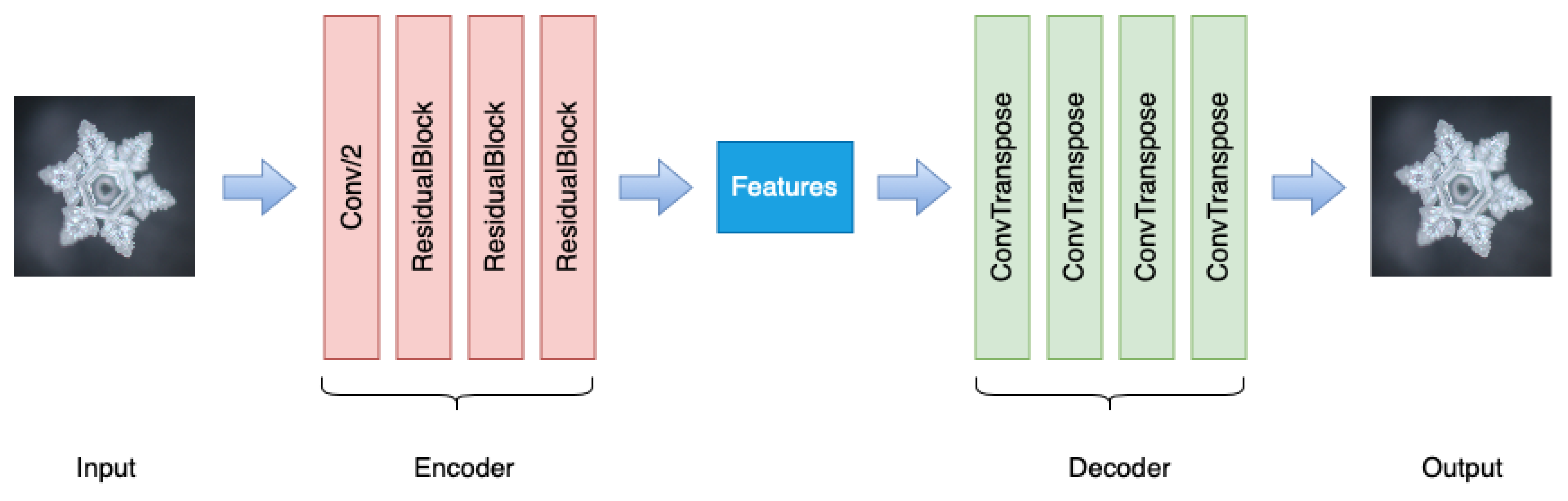
4.1. Feature Extractor
4.1.1. Residual Auto-Encoder
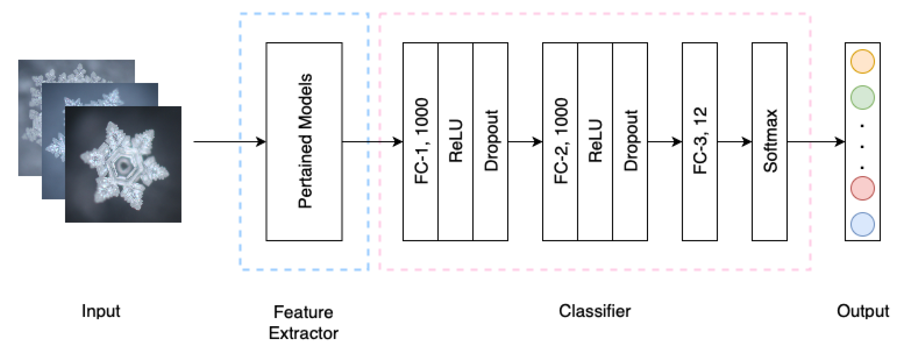
4.1.2. Fine-Tuning Model
4.2. Classification Model
4.3. Imbalanced Data
5. Experiments and Results
5.1. Evaluation Metric
5.1.1. Classification Accuracy
5.1.2. -Score
5.2. Experiments Environment and Setup
5.3. Experiment Results
5.3.1. Residual Auto-Encoder Model (RAE)
5.3.2. Classification Model
5.3.3. Comparative Model
6. Conclusions
Author Contributions
Funding
Informed Consent Statement
Data Availability Statement
Acknowledgments
Conflicts of Interest
References
- Boyd, C.E. Water Quality: An Introduction, 3rd ed.; Springer Nature Switzerland AG: Berlin/Heidelberg, Germany, 2020. [Google Scholar] [CrossRef]
- Pollack, G. The Fourth Phase of Water: Beyond Solid, Liquid and Vapor; Ebner & Sons: Springfield, OH, USA, 2013. [Google Scholar]
- Nakaya, U. Snow Crystals: Natural and Artificial; Hokkaido University: Hokkaido, Japan, 1954. [Google Scholar]
- Magono, C.; Lee, C.W. Meteorological classification of natural snow crystals. J. Fac. Sci. Hokkaido Univ. Ser. 7 Geophys. 1966, 2, 321–335. [Google Scholar]
- Kikuchi, K.; Kameda, T.; Higuchi, K.; Yamashita, A.; Working Group Members for New Classification of Snow Crystals. A global classification of snow crystals, ice crystals, and solid precipitation based on observations from middle latitudes to polar regions. Atmos. Res. 2013, 132, 460–472. [Google Scholar] [CrossRef]
- Hicks, A.; Notaroš, B. Method for Classification of Snowflakes Based on Images by a Multi-Angle Snowflake Camera Using Convolutional Neural Networks. J. Atmos. Ocean. Technol. 2019, 36, 2267–2282. [Google Scholar] [CrossRef]
- Ziletti, A.; Kumar, D.; Scheffler, M.; Ghiringhelli, L.M. Insightful classification of crystal structures using deep learning. Nat. Commun. 2018, 9, 2775. [Google Scholar] [CrossRef] [PubMed] [Green Version]
- Radin, D.; Hayssen, G.; Emoto, M.; Kizu, T. Double-blind test of the effects of distant intention on water crystal formation. Explore 2006, 2, 408–411. [Google Scholar] [CrossRef] [PubMed]
- Radin, D.; Lund, N.; Emoto, M.; Kizu, T. Effects of distant intention on water crystal formation: A triple-blind replication. J. Sci. Explor. 2008, 22, 481–493. [Google Scholar]
- Feng, S.; Zhou, H.; Dong, H. Using deep neural network with small dataset to predict material defects. Mater. Des. 2019, 162, 300–310. [Google Scholar] [CrossRef]
- Masci, J.; Meier, U.; Cireşan, D.; Schmidhuber, J. Stacked convolutional auto-encoders for hierarchical feature extraction. In International Conference on Artificial Neural Networks; Springer: Berlin/Heidelberg, Germany, 2011; pp. 52–59. [Google Scholar]
- Garrett, T.; Fallgatter, C.; Shkurko, K.; Howlett, D. Fall speed measurement and high-resolution multi-angle photography of hydrometeors in free fall. Atmos. Meas. Tech. 2012, 5, 2625–2633. [Google Scholar] [CrossRef] [Green Version]
- Praz, C.; Roulet, Y.A.; Berne, A. Solid hydrometeor classification and riming degree estimation from pictures collected with a Multi-Angle Snowflake Camera. Atmos. Meas. Tech. 2017, 10, 1335–1357. [Google Scholar] [CrossRef] [Green Version]
- Leinonen, J.; Berne, A. Unsupervised classification of snowflake images using a generative adversarial network and K-medoids classification. Atmos. Meas. Tech. 2020, 13, 2949–2964. [Google Scholar] [CrossRef]
- Goodfellow, I.; Pouget-Abadie, J.; Mirza, M.; Xu, B.; Warde-Farley, D.; Ozair, S.; Courville, A.; Bengio, Y. Generative adversarial nets. In Advances in Neural Information Processing Systems; MIT Press: Cambridge, MA, USA, 2014; pp. 2672–2680. [Google Scholar]
- Jain, A.K.; Murty, M.N.; Flynn, P.J. Data clustering: A review. ACM Comput. Surv. (CSUR) 1999, 31, 264–323. [Google Scholar] [CrossRef]
- Emoto, H.; Doan Thi, H.; Andres, F.; Hayashi, M.; Katsumata, K.; Oshide, T.; Tran, L. 5K EPP Dataset 2021. Available online: https://ieee-dataport.org/documents/5k-epp-dataset (accessed on 15 October 2019). [CrossRef]
- Otsu, N. A threshold selection method from gray-level histograms. IEEE Trans. Syst. Man Cybern. 1979, 9, 62–66. [Google Scholar] [CrossRef] [Green Version]
- He, K.; Zhang, X.; Ren, S.; Sun, J. Deep residual learning for image recognition. In Proceedings of the IEEE Conference on Computer Vision and Pattern Recognition, Las Vegas, NV, USA, 27–30 June 2016; pp. 770–778. [Google Scholar]
- Tran, B.; Le Thi, H.A. Deep Clustering with Spherical Distance in Latent Space. In International Conference on Computer Science, Applied Mathematics and Applications; Springer: Berlin/Heidelberg, Germany, 2019; pp. 231–242. [Google Scholar]
- Deng, J.; Dong, W.; Socher, R.; Li, L.J.; Li, K.; Fei-Fei, L. Imagenet: A large-scale hierarchical image database. In Proceedings of the 2009 IEEE Conference on Computer Vision and Pattern Recognition, Miami, FL, USA, 20–25 June 2009; pp. 248–255. [Google Scholar]
- Krizhevsky, A.; Sutskever, I.; Hinton, G.E. Imagenet classification with deep convolutional neural networks. In Advances in Neural Information Processing Systems; MIT Press: Cambridge, MA, USA, 2012; pp. 1097–1105. [Google Scholar]
- Simonyan, K.; Zisserman, A. Very deep convolutional networks for large-scale image recognition. arXiv 2014, arXiv:1409.1556. [Google Scholar]
- Iandola, F.N.; Han, S.; Moskewicz, M.W.; Ashraf, K.; Dally, W.J.; Keutzer, K. SqueezeNet: AlexNet-level accuracy with 50x fewer parameters and <0.5 MB model size. arXiv 2016, arXiv:1602.07360. [Google Scholar]
- Huang, G.; Liu, Z.; Van Der Maaten, L.; Weinberger, K.Q. Densely connected convolutional networks. In Proceedings of the IEEE Conference on Computer Vision and Pattern Recognition, Honolulu, HI, USA, 21–26 July 2017; pp. 4700–4708. [Google Scholar]
- Goutte, C.; Gaussier, E. A probabilistic interpretation of precision, recall and F-score, with implication for evaluation. In European Conference on Information Retrieval; Springer: Berlin/Heidelberg, Germany, 2005; pp. 345–359. [Google Scholar]
- Balouek, D.; Carpen Amarie, A.; Charrier, G.; Desprez, F.; Jeannot, E.; Jeanvoine, E.; Lèbre, A.; Margery, D.; Niclausse, N.; Nussbaum, L.; et al. Adding Virtualization Capabilities to the Grid’5000 Testbed. In Cloud Computing and Services Science; Ivanov, I.I., van Sinderen, M., Leymann, F., Shan, T., Eds.; Communications in Computer and Information Science; Springer International Publishing: Berlin/Heidelberg, Germany, 2013; Volume 367, pp. 3–20. [Google Scholar] [CrossRef]
- Kingma, D.P.; Ba, J. Adam: A method for stochastic optimization. arXiv 2014, arXiv:1412.6980. [Google Scholar]
- Wang, Z.; Bovik, A.C.; Sheikh, H.R.; Simoncelli, E.P. Image quality assessment: From error visibility to structural similarity. IEEE Trans. Image Process. 2004, 13, 600–612. [Google Scholar] [CrossRef] [Green Version]
- Ng, A. Machine Learning Yearning. 2017. Available online: http://www.mlyearning.org/(96) (accessed on 15 October 2019).
- Srivastava, N.; Hinton, G.; Krizhevsky, A.; Sutskever, I.; Salakhutdinov, R. Dropout: A simple way to prevent neural networks from overfitting. J. Mach. Learn. Res. 2014, 15, 1929–1958. [Google Scholar]


| Category | Crystal Example | Definition |
|---|---|---|
| Microparticule |  | Crystal made up of fine particle on a hexagonal plate |
| Simple plate |  | Hexagonal crystal with no outer decoration |
| Fan-like plate | 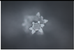 | Square plate with a fan-shaped decoration on the outside |
| Dentrite plate | 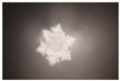 | A square plate with dendritic decoration on the outside |
| Fern-like dendrite plate |  | A square plate with fern-like decorations on the outside |
| Column/Square | 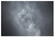 | Square or columnar crystal/block crystal |
| Singular Irregular |  | Square plate with a fan-shaped decoration on the outside |
| Cloud-particle | 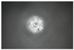 | A granular decoration on a square plate |
| Combinations | 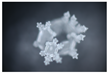 | Multiple square plates assembled together without overlapping vertically |
| Double plate | 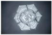 | Two square plates stacked on top of each other |
| Multiple Columns/Squares | 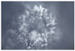 | Multiple square or columnar crystals / Multiple block crystals |
| Multiple Irregulars | 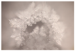 | Multiple asymmetrical crystals or crystals that are not fully formed |
| undefined |  | Types of water crystals without crystals |
| Category | Card(Photo) | Percentage |
|---|---|---|
| Microparticle | 161 | 3.2% |
| Simple plate | 104 | 2% |
| Fan-like plate | 341 | 6.81% |
| Dendrite plate | 1388 | 27.72% |
| Fern-like dendrite plate | 674 | 13.46% |
| Column/Square | 38 | 7.5% |
| Singular Irregular | 674 | 13.46% |
| Cloud-particle | 3 | 0.0006% |
| Combination | 129 | 2.57% |
| Double plates | 204 | 4% |
| Multiple Columns/Squares | 172 | 3.4% |
| Multiple Irregular | 692 | 13.82% |
| Undefined | 427 | 8.52% |
| Backbone | Loss | Accuracy | -Score |
|---|---|---|---|
| RAE | 0.094 | 94.35% | 91.64% |
| AlexNet | 0.086 | 93.71% | 87.79% |
| VGG | 0.049 | 96.21% | 92.03% |
| SqueezeNet | 0.130 | 91.16% | 83.31% |
| DenseNet | 0.046 | 96.93% | 93.55% |
| ResNet | 0.025 | 98.50% | 97.25% |
Publisher’s Note: MDPI stays neutral with regard to jurisdictional claims in published maps and institutional affiliations. |
© 2022 by the authors. Licensee MDPI, Basel, Switzerland. This article is an open access article distributed under the terms and conditions of the Creative Commons Attribution (CC BY) license (https://creativecommons.org/licenses/by/4.0/).
Share and Cite
Thi, H.D.; Andres, F.; Quoc, L.T.; Emoto, H.; Hayashi, M.; Katsumata, K.; Oshide, T. Deep Learning-Based Water Crystal Classification. Appl. Sci. 2022, 12, 825. https://doi.org/10.3390/app12020825
Thi HD, Andres F, Quoc LT, Emoto H, Hayashi M, Katsumata K, Oshide T. Deep Learning-Based Water Crystal Classification. Applied Sciences. 2022; 12(2):825. https://doi.org/10.3390/app12020825
Chicago/Turabian StyleThi, Hien Doan, Frederic Andres, Long Tran Quoc, Hiro Emoto, Michiko Hayashi, Ken Katsumata, and Takayuki Oshide. 2022. "Deep Learning-Based Water Crystal Classification" Applied Sciences 12, no. 2: 825. https://doi.org/10.3390/app12020825
APA StyleThi, H. D., Andres, F., Quoc, L. T., Emoto, H., Hayashi, M., Katsumata, K., & Oshide, T. (2022). Deep Learning-Based Water Crystal Classification. Applied Sciences, 12(2), 825. https://doi.org/10.3390/app12020825