Abstract
Skin cancer treatment is a combination of BRAF and MEK kinase inhibitors administered as tablets, along with immunotherapy treatment (treatment into the vein) with a group of drugs that inhibit the activity of the immune barrier proteins PD-1 and PDL1. Here, we propose a new approach to the therapy for melanoma with the BRAF/MEK inhibitor and anti-PD-1. With the help of explicit analytical functions, we were able to model this combined treatment and present the treatment in a mathematical model described by a system of differential equations including variables, such as Treg, IL12, Il10, TGF-, and cytokine, which are significant variables that are all critical factors which determine the effectiveness of therapies. The most significant advantage of a treatment described by a mathematical model with explicit analytical functions is the control of parameters, such as time and dose, which are variable critical parameters in the treatment, that is, these parameters can be adapted to the patient’s personalized treatment. In the current study, we showed that by simultaneously changing and combining these two parameters, we could decrease the tumor volume. To validate the numerical results, we computed the relative error between the results obtained from the mathematical model and clinical data.
1. Introduction
Melanoma is a rapid growth of melanocyte cells in the skin. This cancerous growth usually starts in the skin or moles. Rarely, it may appear in organs other than the skin, such as the eyeball (extensive information on this subject is provided in a separate chapter below), the oral mucosa, or under the nails. Sometimes, this tumor spreads to other organs in the body through the lymph ducts or the bloodstream. Cancerous growth of the melanoma may appear in the skin and all over the body; however, in women, the most common area for the appearance of melanoma is the skin of calves, and in men, melanoma is more common in the skin of the back [1].
Types of malignant melanoma These include superficially spreading melanoma, nodular melanoma, lentigo maligna melanoma, and acral melanoma. In advanced melanoma, the cancer cells spread from their primary site to other parts of the body, causing another cancerous growth, called a secondary or metastatic cancer. Melanoma spreads to other distant skin areas, distant lymph nodes, lungs, liver, bones, and the brain. Sometimes, advanced melanoma is diagnosed as melanoma that has returned to another part of the body, even many years after the primary melanoma is removed, or when metastatic disease is diagnosed after additional tests are performed after the initial lesion is removed [2].
Symptoms of the disease: Most types of malignant melanoma begin with a change in the skin, such as a new or existing mole that has changed its shape.
Geometry: A mole with an asymmetrical shape.
Border: A mole whose border is not rounded, clear, or defined.
Shade (Color): A mole whose color is not uniform, and consists of several shades, such as brown, black, pink, and more.
Size: A mole exceeding 5 mm in diameter.
Height: Change in height or any change in the previous four sections [3].
Treatment of melanoma is very broad and depends on the stage of the disease. In this section, we will not review all the possibilities of treating the disease but will present those relevant to the current study.
MEK Inhibitors Combined with BRAF Inhibitors for Metastatic Melanoma. These treatments are intended for melanoma at an advanced stage (stage 4, metastatic disease). Patients with melanoma (approximately 40–50 percent) have a mutation in the BRAF gene, which causes uncontrolled cell division and the development of a cancerous tumor. A group of drugs targeting mutations in the BRAF gene neutralizes the mutation and leads to regulated cellular division. These drugs are effective in patients with the BRAF V600E mutation (accounting for 70–80 percent of the BRAF mutation). The MEK gene is closely related to the BRAF gene, and MEK-targeted drugs can treat melanoma with BRAF mutations. It is reported that a combination of a BRAF inhibitor with an MEK inhibitor is more effective in the treatment of melanoma than either type alone [4]. In patients with the BRAF V600K mutation (which accounts for 20–30 percent of BRAF mutations), immunotherapy treatments were more effective. The most common immunotherapeutic drugs to treat melanoma are checkpoint inhibitors that work by releasing T cells—immune cells that can destroy tumors. For example, pembrolizumab is a monoclonal antibody that blocks the activity of the PD-1 protein by binding to its receptor, allowing the body’s immune system to attack melanoma cells [5,6,7,8,9,10,11].
In this study, we present a new personalized treatment protocol for melanoma that combines biological therapy with immunotherapy using a mathematical model. The mathematical model contains analytical functions that depend on parameters and variables that can be changed to control the time of drug administration and dosage.
The purpose of the current study is to propose a treatment protocol for melanoma that is personalized for each patient and differs from the existing standard protocol. The treatment protocol considers changes in the treatment time intervals and dose given to each patient.
2. Medical Assumptions and Mathematical Equations
In this section, we present the assumptions of a mathematical model that considers the correlation between PD-1 inhibitors and BRAF/MEK inhibitors in melanoma therapy [12]. The dynamic variables of the model are as follows: H is the HMGB-1 concentration, is the density of necrotic cancer cells, D is the density of DCs, is the density of activated CD4+T cells, is the density of activated CD8+T cells, is the density of activated Treg cells, M is the density of activated MDSCs, C is the density of cancer cells, concentration, concentration, is the TGF- concentration, concentration, concentration, is the PD-1 concentration, is the PD-L1 concentration, Q is the PD-1-PD-L1 concentration, is the anti-PD-1 concentration, and is the BRAF/MEK inhibitor concentration.
The main medical assumptions of the model are as follows [13,14,15,16,17,18,19,20]: the tumor is spherical, and growth depends on time, and its radius is denoted by ; the total density of cells within the tumor is constant in space and time, that is, ; and the densities of immature dendritic cells and naive CD4+T and CD8+T cells remain constant throughout the tumor tissue. All cells have the same velocity u dependent on space and time, and all cytokines and anti-tumor drugs diffuse within the tumor.
The anti-PD-1 as well as the BRAF/MEK inhibitor are injected intradermally every three days for 30 days [21]. The cells involved in the interaction have approximately the same surface area and volume, and hence, the diffusion coefficients of all these cells are the same. All densities and concentrations are radially symmetric; hence, they are a function of the radial time space .
Let us define the following operators , where ∘ is the dynamical variable of the system (for example, , such that , and , where are the dynamical variables of the system, for example . In addition, we define the inhibition by IL-10 as , the inhibition by Tregs as , and the inhibition by PD-1-PD-L1 as .
The dynamic variables of the system (in units of g/cm) are as follows:
HMGB-1 concentration;
density of necrotic cancer cells;
Density of DCs;
density of activated T cells;
density of activated T cells;
density of activated Treg cells;
density of activated MDSCs;
density of cancer cells;
IL-12 concentration;
IL-2 concentration;
TGF- concentration;
IL-6 concentration;
IL-10 concentration;
PD-1 concentration;
anti-PD-1 concentration;
BRAF/MEK inhibitor concentration;
tumor radius;
cell velocity.
The operators , contain two mathematical terms. The first one, , expresses velocity, and the second one, , expresses diffusion.
Under the above assumptions, the mathematical model includes nonlinear partial differential equations in the following form:
Equation for DCs (D)
Biological interpretation of the mathematical expressions is as follows: , released from necrotic cancer cells; , degradation; and , the life of cancer cells.
Dendritic cells are activated by HMGB-1
The expression describes the activation of dendritic cells by HMGB-1, and describes the death of dendritic cells.
Equation for cells and
The expressions in the RHS of these equations are the first terms describe the activation by IL-12, the inhibition by IL-10, and Treg. All these expressions are multiplied by the factor , which describes inhibition by PD-1-PD-L1. The second term is IL-2-induced proliferation, and the last term is the death of and cells.
Equation for activated Tregs
The term is the -induced proliferation, is the activated Tregs recruited into the tumor by tumor-derived immunosuppressive cytokine IL-6, and the last term describes the death of Tregs.
Equation for activated MDSCs
The term describes the MDSCs that are chemotactically attracted to the tumor microenvironment by IL-6, and is the death of MDSC.
Equation for tumor cells
The expression is the proliferation of cancer cells, the term is the inhibition by BRAF/MEKi, the term describes the killing by T cells, and the last term is the death of tumor cells.
Equation for IL-12
The first term is the production by DCs, and the second term is the degradation of IL-12.
Equation for IL-2
The first term is the production by T1, and the second term is the degradation of IL-2.
Equation for TGF-
The term is the production by cancer cells, is the production by Tregs, is the production by MDSCs, and is the degradation of TGF-.
Equation for IL-6
The first term describes the production of IL-6 by cancer cells, and the second term is the degradation of IL-6.
Equation for IL-10
The term represents the production of IL-10 by cancer cells, is the production of IL-10 by MDSCs, and is the degradation of IL-10.
Equation for PD-1, PD-L1 and PD-1-PD-L1
where . PD-1 is expressed on the surface of activated cells, activated cells, and Tregs. The mathematical relationship between the number of PD-1 and and is proportional to the factor (it is constant when no anti-PD-1 drug is administered), and the number of PD-1 is smaller than Treg by the factor .
In addition, PD-L1 is expressed on the surface of activated cells, activated cells, MDSCs, and tumor cells. The mathematical connection between the number of PD-L1 and , and is proportional to the factor , and the number of PD-L1 is smaller than that of C cells by the factor and smaller than that of the M cells by the factor ; hence, .
Equation for anti-PD-1
where is the treatment of anti PD-1, is the depletion through blocking PD-1, is the degradation of anti PD-1.
Equation for BRAF/MEK inhibitor
where is the treatment of BRAF/MEK, is the absorption of BRAF/MEKi by cancer cells, and is the degradation of the BRAF/MEK inhibitor.
Equation for cells velocity
The treatment is biological, assuming all the cells have the same volume and surface area, the diffusion of all the cells are the same.
Equation for free boundary
We assumes that the free boundary moves with the velocity of cells.
The boundary conditions of the model are as follows ( flux conditions at the tumor boundary):
The initial conditions of the model are as follows:
The following analytical functions represent the biological and immunotherapy treatment protocols, with the parameter q describing the dose, and variable t representing the time interval. These two parameters can be changed, that is, they are customizable parameters.
3. Results and Discussion
In this section, we present the results obtained by solving the mathematical models (1)–(18) (under the boundary and initial conditions (19) and (20)) using the functions (21) and (22) for different dosages q and time intervals t. The parameters for numerical simulations are presented in the tables in the Appendix A section.
We solved the mathematical model using the MATLAB PDE solverfor initial-boundary value problems for PDE systems. We applied different combinations of treatments using functions (21) and (21). Figure 1, Figure 2, Figure 3, Figure 4, Figure 5, Figure 6 and Figure 7 present examples of our results.
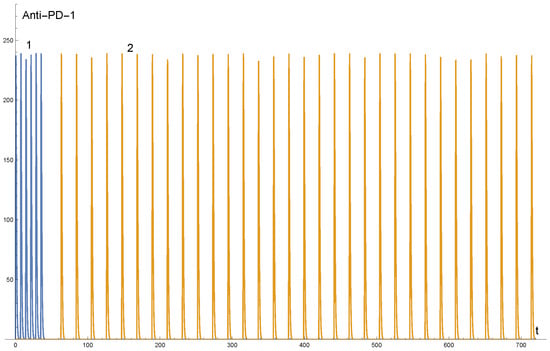
Figure 1.
The y-axis represents the dosage of the ANTI PD-1 treatment and x-axis represents the time in days. The given dosage is 3 mg per kg. This figure presents a treatment for a patient weighing 82 kg. The scheduled administration and doses were: once a week infusion into the vein for 7 weeks, break in the treatment for 3 to 4 weeks, and then the treatment was repeated once a week. The dose was 242 mg each time. Line 1 presents the first period of treatment, that is, the first 7 weeks, and line 2 presents the second period of treatment.
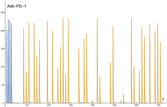
Figure 2.
The y-axis represents the dosage of the ANTI PD-1 treatment and x-axis represents the time in days. The doses and the time of administration of the drug varied.
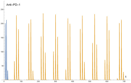
Figure 3.
The y-axis represents the dosage of the ANTI PD-1 treatment, and x-axis represents the time in days. The doses and the time of administration of the drug varied.
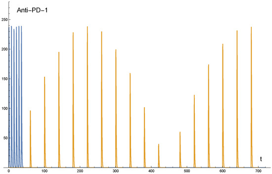
Figure 4.
The y-axis represents the dosage of the ANTI PD-1 treatment and x-axis represents the time in days. The doses and the time of administration of the drug varied.
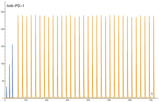
Figure 5.
The y-axis represents the dosage of the ANTI PD-1 treatment and x-axis represents the time in days. At the first period of the treatment, the dosages varied in time, and at the second period of the treatment, the dosages were fixed.
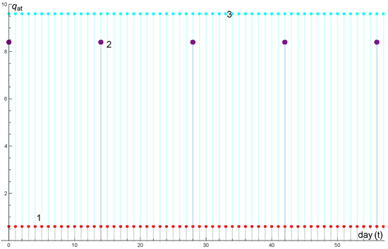
Figure 6.
The y-axis (divided by 100) represents the dosage of the drug and x-axis represents the time in days. Discrete plot 1: drug: cobimetinib, 60 mg. Discrete plot 2: drug: atezolizumab, 840 mg. Discrete plot 3: drug: vemurafenib, 960 mg.
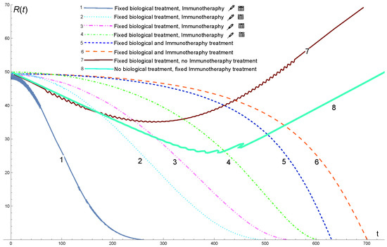
Figure 7.
Solution profiles of the mathematical model for different combinations of treatment, that is, biological and immunotheraphy treatments. The injector drawing indicates varying doses, and the calendar drawing indicates that the times vary.
Figure 1 presents the function of anti , which is an example of the protocol treatment. Function depends on the time and dose. Both these parameters can be changed to customize the treatment. This figure presents only one combination of protocols, that is, a fixed schedule of administration and doses. The standard treatment was as follows: once a week, infusion into the vein for 7 weeks at a dose of 3 mg per kg. After that, there was a break in the treatment for 3–4 weeks, and the treatment was repeated once a week. This treatment was administered for 24 months.
All immunotherapeutic protocols in our numerical simulation were divided into two periods: once-a-week infusion into the vein for 7 weeks with q mg per kg. After that, there was a break in the treatment for 3–4 weeks, and the treatment was repeated once a week. This treatment was administered for 24 months. The minimum dosage was 0.9 mg per kg, and the maximum dosage was 3 mg per kg.
Figure 6 shows an example of the following treatment protocol.
Drug: Vemurafenib;
Dosage and schedule: 960 mg twice daily during the run-in phase, followed by 720 mg twice daily;
Drug: Cobimetinib;
Dosage and schedule: 60 mg once daily;
Drug: Atezolizumab;
Dosage and schedule: 840 mg every 2 weeks.
Figure 7 shows the solution profiles of the mathematical model for different combinations of treatment. Line 7 presents a treatment that includes only a biological protocol without immunotherapy, that is, the function and . As shown in the graph, the tumor decreased from the initial conditions (initial treatment) during the ≈300 days of treatment, after which the tumor grew.
Figure 7 line 8 presents a treatment that includes only immunotherapy without biological treatment, that is, the function and . As shown in the graph, the tumor decreased from the initial conditions (initial treatment) during the ≈400 days of treatment, after which the tumor grew.
Figure 7 lines 5 and 6 present a combination of biological treatment and immunotherapy (no changes in time and dosage), that is, , the standard protocol. The protocol for biological treatment is presented in function (22). The immunotherapy protocol was as follows: for line 5, 1 mg per kg fixed interval and dosage during the entire treatment period; and for line 6, 1.42 mg per kg fixed interval and dosage during the entire treatment period. As can be seen from these results the tumor, in both cases, it decreases very slowly.
Figure 7 line 1 presents the optimal treatment because the tumor decreased to zero very quickly compared to the other treatment protocols. The protocol was a combination of biological and immunotherapy treatments. The biological treatment had a fixed time and dosage, as presented in function (22). The immunotherapy treatment differed from the standard protocol. In this case, we defined the treatment so that it varies in terms of the administration of the drug and also the dose (see Figure 2). The change in the dose and time of drug administration was not arbitrary, but in the following order: after the initial treatment (that is, solving the mathematical model with the boundary and initial conditions), we extracted the vector of the model’s results and defined it as the initial conditions and boundary conditions for the mathematical model, in order for the initial conditions to change and not be fixed as usual when solving a system of differential equations (the standard method to solve a system of ODE, PDE with an initial condition is that the initial condition is fixed and does not change in time). In this method, in fact, the mathematical model is updated at any given moment regarding the size of the tumor and thus the dose changes according to the size of the tumor. For example, if the size of the tumor increases during treatment, then the dose will increase accordingly, and if the size of the tumor decreases during treatment, then the dose will decrease accordingly.
Figure 7 line 2 presents a combination of biological treatment and immunotherapeutic treatments (see Figure 3). The biological treatment was fixed, as present in function (22). The immunotherapy treatment in this case was cyclical during both periods of treatment (according to the above comment). The treatment varies in terms of time, meaning that it is not given at fixed times but is given in cycles of treatment. The dose is also variable and not fixed, that is, the dose changes cyclically. In this case, we observed that the cancerous tumor decreased to zero but only after 480 days of combined treatment.
Figure 7 line 3 presents a combination of biological treatment and immunotherapy (see Figure 4). Biological treatment is a fixed treatment. The immunotherapy treatment in the first period was the same as the standard treatment, meaning a fixed dose and fixed treatment times (i.e., once a week infusion into the vein for 7 weeks with a dose of q milligrams per 1 kilogram). However, in the second period, the dose and treatment times changed cyclically. Initially, the dose was increased up to 220 days, after which the dose was decreased to almost zero for another 220 days and so on. In this case, the growth dropped to zero after 540 days.
Figure 7 line 4 presents a combination of biological treatment and immunotherapy such that the biological is the standard protocol, and the immunotherapy treatment changes as follows (see Figure 5): in the first period of 7 weeks, the treatment varied in terms of the dose but was given at fixed interval times, and in the second period of the treatment, the doses and the time interval of the treatments were fixed throughout the rest of the treatment time. In this case, we observed that the size of the cancer tumor decreased only after 600 days.
Relative Error Analysis
In this section, we compute the relative error between the results obtained from the mathematical model for the standard protocol, with the clinical results obtained from the open access NIH U.S. national Library of Medicine [22]. To this end, we define the following expressions:
i.e., the index 6 refers to numerical plot number 6 from Figure 7, and 5 refers to numerical plot number 5 from Figure 7. It should be noted that the data shown in these graphs (Figure 8 and Figure 9) are discrete and not continuous, so we must extract the information about the size of the tumor from the numerical mathematical solution for comparison with the clinical data.
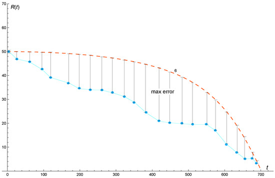
Figure 8.
Comparison of results between the solution profile of the mathematical model with the standard protocol and clinical data. The dashed line represents the plot obtained from the mathematical model (see plot number 6 from Figure 7) and the dot plot represents the clinical data obtained from the open access data: https://www.clinicaltrials.gov/, accessed on 25 September 2022.
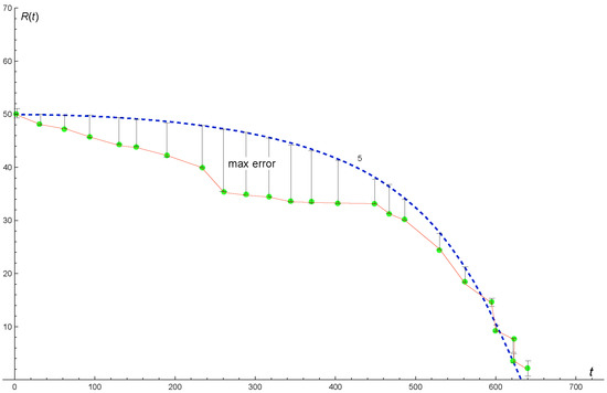
Figure 9.
Comparison of results between the solution profile of the mathematical model with the standard protocol and clinical data. The dashed line represents the plot obtained from the mathematical model (see plot number 5 from Figure 7) and the dot plot represents the clinical data obtained from the open access data: https://www.clinicaltrials.gov/, accessed on 25 September 2022.
According to our analysis, we obtained that and . This means that the maximum relative error is between 0 and percent for the standard protocol of plot 6 and the maximum relative error is between 0 and percent for the standard protocol of plot 5.
4. Conclusions
In the current study, we investigated an innovative treatment for melanoma that includes biological therapy and immunotherapy. The research was conducted using a mathematical model that included a combined system of partial and ordinary differential equations. We modeled the treatment of melanoma using two analytical functions. One function for the anti PD-1, PD-L1, and biological treatment, and one function for the BRAF/MEK inhibitor. These two functions depend on two parameters: dose of the drug and time interval. These two parameters can be controlled so that the treatment is personalized. We solved the mathematical model for different combinations of treatments. We considered changes in different periods of time and doses. We solved the model each time for different combinations of treatments. Through numerical simulations, we discovered that the optimal treatment in which the cancer drops to zero the fastest is a combined treatment of biological treatment and immunotherapy so that the biological treatment is the standard treatment, that is, giving a drug in equal and fixed periods of time and the same amount of medicine in every treatment. However, immunotherapy treatment is not fixed in terms of time and dose. The time periods were not fixed, and the dosage varied from treatment to treatment. To differentiate from other combinations of the immunotherapy treatment where although the doses were not fixed, they were of a cyclical nature and so were the periods of time between treatments.
In addition, we compared our numerical results to clinical data for the standard protocol. We defined the relative error related to the numerical solutions and we found that the maximal gap between these results and data was between 0 and .
Author Contributions
Methodology, O.N. and M.S. Numerical simulations and application of algorithm, O.N. All authors have read and agreed to the published version of the manuscript.
Funding
This research received no external funding.
Institutional Review Board Statement
OPhir nave nd Moriah Sigron: Jerusalem College of Technology, Academic Lev Center Jerusalem, Israel.
Informed Consent Statement
Informed consent was obtained from all subjects involved in the study.
Data Availability Statement
Not applicable.
Conflicts of Interest
The authors declare no conflict of interest.
Appendix A
The following parameters were used for the analysis [12]:
| Parameter | Description | Value and Units |
| Diffusion coefficient of DCs | cmday | |
| Diffusion coefficient of T cells | cmday | |
| Diffusion coefficient of MDSCs | cmday | |
| Diffusion coefficient of tumor cells | cmday | |
| Diffusion coefficient of | cmday | |
| Diffusion coefficient of | cmday | |
| Diffusion coefficient of | cmday | |
| Diffusion coefficient of | cmday | |
| Diffusion coefficient of | cmday | |
| Diffusion coefficient of anti- | cmday | |
| Diffusion coefficient of BRAF/MEK | cmday | |
| Flux rate of and cells at the boundary | 1 cm | |
| Chemoattraction coefficient of | 10 cm/g· day | |
| Production rate of by | day | |
| Production rate of by MDSCs | day | |
| Production rate of by cancer cells | day | |
| Production rate of by cancer cells | day | |
| Production rate of by MDSCs | day | |
| Production rate of by MDSCs | day | |
| Production rate of by cells | day | |
| Growth rate of cancer cells uninhibited (by immune cells) | day | |
| Production rate of by cancer cells | day | |
| Activation rate of MDSCs | day | |
| Growth rate of cancer cells | day | |
| Production rate of by DCs | day | |
| Production of by BRAF/MEKi | 1 | |
| Activation rate of by | day | |
| Activation rate of DCs by tumor cells | 4 g/cm day | |
| Activation rate of cells by | day | |
| Activation rate of cells by | day | |
| Activation rate of cells by | day | |
| Activation rate of by | day | |
| Killing rate of tumor cells by cells | day cm/g | |
| Killing rate of tumor cells by cells | 46 day cm/g | |
| Blocking rate of by anti- | cm/g· day | |
| Absorbtion rate of BRAF/MEKi by cancer cells | day | |
| Expression of in T cells | ||
| Expression of in T cells | ||
| Expression of in tumor cells | ||
| Expression of in MDSCs | day | |
| Death rate of DCs | day | |
| Death rate of cells | day | |
| Death rate of cells | day | |
| Death rate of Tregs | day | |
| Death rate of MDSCs | day | |
| Death rate of tumor cells | day | |
| Degradation rate of | day | |
| Degradation rate of | day | |
| Degradation rate of | day | |
| Degradation rate of | day | |
| Degradation rate of | day | |
| Degradation rate of anti- | day | |
| Degradation rate of BRAF/MEKi | day | |
| Density of inactive DCs | g/cm | |
| Density of naive cells in tumor | g/cm | |
| Density of naive cells in tumor | g/cm | |
| CM | Carrying capacity of cancer cells | g/cm |
| Density of cells from lymph node | g/cm | |
| Density of cells from lymph node | g/cm | |
| Half-saturation of cells | g/cm | |
| Half-saturation of cells | g/cm | |
| Half-saturation of Tregs | g/cm | |
| Half-saturation of tumor cells | g/cm | |
| Half-saturation of | g/cm | |
| Half-saturation of | g/cm | |
| Half-saturation of | g/cm | |
| Half-saturation of | g/cm | |
| Half-saturation of | g/cm | |
| Half-saturation of | g/cm | |
| Half-saturation of BRAF/MEKi | g/cm | |
| Inhibition of function of T cells by | g/cm | |
| Inhibition of proliferation of cancer cells by BRAF/MEKi | g/cm |
References
- Israel Cancer Association. Available online: https://www.cancer.org.il/ (accessed on 25 September 2022).
- MAYO CLINIC. Available online: https://www.mayoclinic.org/diseases-conditions/melanoma/symptoms-causes/syc-20374884 (accessed on 25 September 2022).
- National Health Service (NHS). Available online: https://www.nhs.uk/conditions/melanoma-skin-cancer/symptoms/ (accessed on 25 September 2022).
- Memorial Sloan Kettering Cancer Center. Available online: https://www.mskcc.org/cancer-care/types/melanoma/treatment/targeted-therapy-melanoma (accessed on 25 September 2022).
- Ghate, S.; Ionescu-Ittu, R.; Burne, R.; Ndife, B.; Lalibert, F.; Nakasato, A.; Duh, M.S. Patterns of treatment and BRAF testing with immune checkpoint inhibitors and targeted therapy in patients with metastatic melanoma presumed to be BRAF positive. Melanoma Res. 2019, 29, 301–310. [Google Scholar] [CrossRef] [PubMed]
- Haist, M.; Stege, H.; Ebner, R.; Fleischer, M.I.; Loquai, C.; Grabbe, S. The Role of Treatment Sequencing with Immune-Checkpoint Inhibitors and BRAF/MEK Inhibitors for Response and Survival of Patients with BRAFV600-Mutant Metastatic Melanoma A Retrospective, Real-World Cohort Study. Cancers 2022, 14, 2082. [Google Scholar] [CrossRef] [PubMed]
- Lelliott, E.J.; McArthur, G.A.; Oliaro, J.; Sheppard, K.E. Immunomodulatory Effects of BRAF, MEK, and CDK4/6 Inhibitors: Implications for Combining Targeted Therapy and Immune Checkpoint Blockade for the Treatment of Melanoma. Front. Immunol. 2021, 12, 661737. [Google Scholar] [CrossRef] [PubMed]
- Pires da Silva, I.; Zakria, D.; Ahmed, T.; Trojanello, C.; Dimitriou, F.; Allayous, C.; Gerard, C.; Zimmer, L.; Lo, S.; Michielin, O.; et al. Efficacy and safety of anti-PD1 monotherapy or in combination with ipilimumab after BRAF/MEK inhibitors in patients with BRAF mutant metastatic melanoma. J. Immunother. Cancer 2022, 10, e004610. [Google Scholar] [CrossRef] [PubMed]
- Van Breeschoten, J.; Wouters, M.W.J.M.; Hilarius, D.L.; Haanen, J.B.; Blank, C.U.; Aarts, M.J.B.; van den Berkmortel, F.W.P.J.; de Groot, J.-W.B.; Hospers, G.A.P.; Kapiteijn, E.; et al. First-line BRAF/MEK inhibitors versus anti-PD-1 monotherapy in BRAFV600-mutant advanced melanoma patients: A propensity-matched survival analysis. Br. J. Cancer 2021, 124, 1222–1230. [Google Scholar] [CrossRef] [PubMed]
- Yan, C.; Chen, S.-C.; Ayers, G.D.; Nebhan, C.A.; Roland, J.T.; Weiss, V.L.; Johnson, D.B.; Richmond, A. Proximity of immune and tumor cells underlies response to BRAF/MEK-targeted therapies in metastatic melanoma patients. Npj Precis. Oncol. 2022, 6, 6. [Google Scholar] [CrossRef] [PubMed]
- Ribas, A.; Algazi, A.; Ascierto, P.A.; Butler, M.O.; Chandra, S.; Gordon, M.; Hernandez-Aya, L.; Lawrence, D.; Lutzky, J.; Miller, W.H., Jr.; et al. PD-L1 blockade in combination with inhibition of MAPK oncogenic signaling in patients with advanced melanoma. Nat. Commun. 2020, 11, 6262. [Google Scholar] [CrossRef] [PubMed]
- Lai, X.; Friedman, A. Combination therapy for melanoma with BRAF/MEK inhibitor and immune checkpoint inhibitor: A mathematical model. BMC Syst. Biol. 2017, 11, 70. [Google Scholar] [CrossRef] [PubMed]
- Tran Janco, J.M.; Lamichhane, P.; Karyampudi, L.; Knutson, K.L. Tumor-Infiltrating Dendritic Cells in Cancer Pathogenesis. J. Immunol. 2015, 194, 2985–2991. [Google Scholar] [CrossRef] [PubMed]
- Saenz, R.; Futalan, D.; Leutenez, L.; Eekhout, F.; Fecteau, J.F.; Sundelius, S.; Sundqvist, S.; Larsson, M.; Hayashi, T.; Minev, B.; et al. TLR4-dependent activation of dendritic cells by an HMGB1-derived peptide adjuvant. J. Transl. Med. 2014, 12, 211. [Google Scholar] [CrossRef] [PubMed]
- Ma, Y.; Shurin, G.V.; Peiyuan, Z.; Shurin, M.R. Dendritic Cells in the Cancer Microenvironment. J. Cancer 2013, 4, 36–44. [Google Scholar] [CrossRef] [PubMed]
- Kawakami, Y.; Yaguchi, T.; Sumimoto, H.; Kudo-Saito, C.; Iwata-Kajihara, T.; Nakamura, S.; Tsujikawa, T.; Park, J.H.; Popivanova, B.K.; Miyazaki, J.; et al. Improvement of Cancer Immunotherapy by Combining Molecular Targeted Therapy. Front. Oncol. 2013, 3, 136. [Google Scholar] [CrossRef] [PubMed]
- Palucka, K.; Banchereau, J. Cancer immunotherapy via dendritic cells. Nat. Rev. Cancer 2012, 12, 265–277. [Google Scholar] [CrossRef] [PubMed]
- Perrot, C.Y.; Javelaud, D.; Mauviel, A. Insights into the Transforming Growth Factor-β Signaling Pathway in Cutaneous Melanoma. Ann. Dermatol. 2013, 25, 135. [Google Scholar] [CrossRef] [PubMed]
- Oelkrug, C.; Ramage, J.M. Enhancement of T cell recruitment and infiltration into tumours. Clin. Exp. Immunol. 2014, 178, 1–8. [Google Scholar] [CrossRef] [PubMed]
- Whiteside, T. The role of regulatory T cells in cancer immunology. ImmunoTargets Ther. 2015, 4, 159. [Google Scholar] [CrossRef] [PubMed]
- Hu-Lieskovan, S.; Mok, S.; Homet Moreno, B.; Tsoi, J.; Robert, L.; Goedert, L.; Pinheiro, E.M.; Koya, R.C.; Graeber, T.G.; Comin-Anduix, B.; et al. Improved antitumor activity of immunotherapy with BRAF and MEK inhibitors in BRAF V600E melanoma. Sci. Transl. Med. 2015, 7, 279ra41. [Google Scholar] [CrossRef]
- U.S. National Library of Medicine. Available online: https://www.clinicaltrials.gov/ct2/home (accessed on 2 November 2022).
Publisher’s Note: MDPI stays neutral with regard to jurisdictional claims in published maps and institutional affiliations. |
© 2022 by the authors. Licensee MDPI, Basel, Switzerland. This article is an open access article distributed under the terms and conditions of the Creative Commons Attribution (CC BY) license (https://creativecommons.org/licenses/by/4.0/).