The Bernoulli Assembly Line: The Analytical and Semi-Analytical Evaluation of Steady-State Performance

Abstract

Assembly lines are one of the cornerstones of modern production systems, significantly affecting the global society, economy, and other ancillary sectors. This is why the evaluation of assembly lines is particularly significant. Hence, the research on modeling approaches is presented in this paper, yielding an efficient mathematical tool that enables the evaluation of the steady-state performance of assembly lines at low CPU cost. First, the analytical model and the transition matrix were developed for the general case, and second, dimensionality issues and demanding computational requirements were tackled by applying the finite state method. Both approaches were employed in different theoretical cases in order to validate the finite state method against the analytical solution. Additionally, the developed evaluation framework was applied in the case of a realistic assembly system, and the obtained results were successfully validated against the factory floor measurements. The comparison of the obtained results proves the finite state method as a reliable and CPU-efficient method, suitable for the evaluation of its key performance indicators as well as implementation within more sophisticated design procedures. This kind of predictive analytics is intended to support production management and enhance the reliability of long- and short-term decision-making in the context of the digital twinning of production systems.

1. Introduction

Today’s global society significantly depends on production, which affects global markets and supply chains, transport systems, local commerce, state economies and policies, our daily routines and habits, social relationships, quality of life, scientific research and development, education, the environment and biodiversity, to name a few. It is a sophisticated and delicate process with the potential to bring societal norms from conventional to new and unprecedented frontiers including its positive and potentially negative consequences at the local and global levels. According to the World Bank, the share of the manufacture of merchandise exports and imports in 2020 amounted to 70.11% and 70.62%, respectively, which is closely related to the service sector, strictly following the evolution of manufacture at the global level [1]. Consequently, any improvement or deterioration in the manufacturing sector has repercussions on a broad spectra of society and its work-force. This is particularly evident if a value of an estimated USD 115 billion is attributed to the export of the manufacturing services of countries such as China, Vietnam, Philippines, the United Kingdom, Japan, Norway, political unions such as the European Union, and others [2]. Simultaneously, production systems are exposed to numerous external (market demands, material supply, financial markets, workforce availability, energy supply, information disruption) and internal (machine failures, storage capacities, cycle time, production quality, rework demands) factors of a predominantly stochastic nature [3]. Therefore, production systems may be considered as inherently stochastic, requiring a suitable mathematical approach that will enable their improvement, design, and management, while at a same time being governed by the principle of profit increase. Such mathematical models have been considered for many years by the production system engineering community [4].

Production systems include the different arrangements of machines, work stations, buffers, and transport devices. Some of the most representative ones are the serial production line, production lines with the splitting of material flow, lines with rework and quality control, lines with assembly operations, or any of their combinations. In such a context, the assembly system represents a production process in which different elements are sequentially added until an end product is created. Therefore, assembly systems involve at least two serial lines and one merging operation, yielding assembled parts delivered for further production activities or, conversely, end products [5]. Depending on the nature of the production process, the product either moves through the production system or is kept stationary in cases when it is of a large scale. In the former case, the machinery and working stations are strictly arranged and kept stationary, while in the latter, workers perform sequential assembly operations according to a predefined layout. Thus, assembly systems are sometimes characterized as concurrent processes (i.e., as multiple parallel production activities) that add value to parts and provide intermediate products to a following or final assembly stage.

Starting with the Industrial Revolution, assembly systems were considered as one of the first mass-production enablers, simultaneously enhancing production efficiency and profit margins, while introducing product quality, reliability, and uniformity. This would consequently be reflected in the development of new management strategies. In addition, the specialization of various work-stations along the assembly line contributed to the standardization of working procedures, the employment of low-wage personnel, and the simpler replacement of departing employees. Therefore, assembly systems often became considered as a company’s growth indicator, standing alongside serial production lines as the workhorse of the industry [4,6]. However, rather expensive production assets came to be associated with the introduction of new assembly systems including demanding management and production organizations, considerable warm-up stages, and additional investments through dedicated education, labor, or factory space [7]. Hence, a rational approach to the problem of assembly system evaluation including the communication between work-stations, material flow plans, and work schedules is a necessary prerequisite, underpinning the companies’ strategic decisions and opening new perspectives of business development. Otherwise, an eventual failure in the system could seriously affect the production process through slowdowns and ineffectiveness, manifested as starvations, blockages, and finally, decreased production rates [8].

Usually, the effectiveness of a particular production system is expressed in terms of the key performance indicator (KPI) for each element of the production system, while the more general concept of overall equipment effectiveness (OEE) is taken into account when considering losses at a systemic level. Both KPI and OEE are of great significance when implementing the lean philosophy principle, particularly in the context of value stream mapping [9]. From a general perspective, KPIs can be classified as quantitative or qualitative values, reflecting objective and measurable facts as well as personal opinions or interpretations. Quantitative KPIs are of particular importance in the context of production system engineering, and these can be categorized into four groups related to revenue, production cost, process improvements, and customer satisfaction. A list of relevant KPIs and their further classification is presented in detail by [10]. Aside from KPIs, the OEE plays a significant role in modern production system management, as a framework providing classification, measurement, and the minimization of production losses and, thus, an increase in effectiveness [11]. The OEE is a measure of the production system’s efficiency, based on a ratio of T_I/T_R, where T_I is the time required for the manufacture of high quality products in ideal conditions, and T_R is the time required for their manufacture in realistic conditions, taking into account the production system availability, breakdowns, scheduled maintenance, defective parts, rework requirements, material supply uncertainties, financial capability, and others [10]. These may be considered as deterministic or stochastic variables and thus will have an impact on the reliability of OEE estimates.

The evaluation of KPIs and OEE requires the application of suitable mathematical models, particularly when variables of a stochastic nature are considered. Some examples include queuing networks, process algebra, Petri nets, or stochastic automata. However, the Markov chain theory is employed as a reliable approach in most cases, yielding joint probability distributions, reflecting the likelihoods of systems in certain states [4]. This approach has therefore been the main focus of the majority of research publications and papers, especially those primarily addressing issues related to serial production lines including different machine reliability definitions. Other line arrangements such as ones including material flow splitting, assembly systems, or lines with reworking stations and quality control have been considered to a significantly smaller extent. This is particularly valid in the case of assembly production lines that are dominantly evaluated through a reduction in the Markovian framework, due to the so-called “dimensionality curse”, to semi-analytical methods such as the aggregation procedure [12] and the decomposition method [13].

Therefore, the major goal of this paper is to present an analytical model of the Bernoulli assembly production line using the Markovian framework through the concept of the generalized transition matrix [14]. This approach will yield an analytically formulated joint probability distribution of a system being in a certain state, which may be used to directly evaluate associated KPIs such as the production rate, work-in-process, and the probabilities of blockage/starvation in the case of an assembly system. Additionally, the state space dimensionality issue is tackled by the finite-state method (FSM). The finite-state method has previously been successfully applied as a reliable, fast, and analytically based method in the case of serial production lines and lines involving the splitting of material flow. Here, and for the first time, it will be extended and validated in relation to assembly lines.

1.1. Brief Literature Review

The simulation of manufacturing systems has continuously attracted attention from researchers and professionals, particularly in the context of digitalization, which has become a cornerstone of factories of the future. It has, thus, become an avenue of new and challenging research, ranging from conventional manufacture to emerging technologies such as the Internet of Things, cyber-physical systems, augmented and virtual realities, digital twinning, and others. However, the majority of research activities have recognized this approach as an excellent tool for the increase in production capacity, while simultaneously controlling the production costs, time, quality, energy efficiency, and finally productivity, particularly in the context of complex manufacturing systems [15]. Indeed, the main goal of this highly emerging field is the development of methodologies for the evaluation of KPIs in the context of process simulation, continuous improvements, quality maintenance, and production system design. While numerous advances have been achieved recently throughout production system engineering [4], this paper will focus on issues of the assembly line considered in the present literature to a considerably lesser extent compared to, for example, serial lines.

The first approximating model of the assembly system was presented in [16], providing a method for the evaluation of the performance of transfer lines with finite inventory banks, typical for the automobile industry. This was followed by the development and application of the decomposition approach, based on a system’s flow conservation principle [17]. Similarly, the approximate evaluation of the production rate and work-in-process was considered in [18] in the case of discrete and continuous flow through the assembly system as an extension of the transfer line theory. An extension of the aggregation procedure and its application in the case of the improvability of the simplest assembly station was presented in [19] including an evaluation of the performance measures and bottleneck identification as well as constrained and unconstrained improvability aspects. This approach has been extended to more general cases such as in [20] and later in [12]. Assembly systems composed of machines of exponential reliability and of different cycle times were presented and evaluated using the decomposition technique in [13], while multiple failure modes were considered in [21] in the same context. Stability conditions, state probabilities, stockout probability, and availability as well as the expected times of failure of an assembly system, composed of two working stations and one merging operation, were elaborated analytically in [22] including an insight into various performance indices. Similarly, the exact solution of a three-station one-buffer assembly system was presented in [23], which included unreliable machines and a definition of the transition matrix. The research efforts focused on topics such as integrated quality and production control [24,25], assembly systems with non-exponential machines [26], the preventive maintenance of assembly systems [27], lead time evaluation [28], multi-product assembly systems [29], or transient response evaluation [30].

However, all of the outlined research efforts and contributions rely predominantly on the application of the decomposition method or the aggregation procedure. The main reason for this is the lack of clear formulation of the transition matrix in the general case of an assembly line, composed of an arbitrary number of machines and buffers of arbitrary capacities. Thus, the same issue (curse of dimensionality), as in the case of serial lines, presents the main obstacle for formulating an analytical solution of the problem [14]. This problem had already been addressed in 1962 in the work of Sevast’yanov, where an approach based on integral equations was employed. However, the obtained system of equations turned out to be complex to the point that its closed-form solution could not be retrieved for the general case. Therefore, the problem was reduced to two random variables, and an associated analytical solution was formulated [31]. As the reach of such a solution is well below practical needs, many researchers (mostly originating from the field of operations’ research and bioinformatics) have developed alternative methods and algorithms through tackling large-scale and dense transition systems. Examples include the decomposition method, aggregation procedure, external memory storage (storing complete transition matrix), selective matrix criteria, state lumping, and sparse matrix approximation [6].

The decomposition method assumes that a large-scale random system may be represented by the decomposition of its state space into multiple communicating classes, with characteristic probability distributions summarizing the behavior of the original system [32]. The applicability of the method was demonstrated in several production lines by addressing various performance measures. The need for more rigorous verification using analytical results was pointed out in [33,34,35]. An opposite approach to the problem of dense and large-scale random systems was applied in the case of the aggregation procedure through the reduction in the system’s state space into a single class of states and the evaluation of the associated probability distribution. This procedure was first introduced in [36] in the research on the simple and analytical modeling of traditional production lines. The method has demonstrated accuracy and validity for application in modern mass-production industry and its main feature is the modeling simplicity and low computational burden.

Apart from operations research, the issue of state-and transition-rich random processes was discussed in [37], following [38] in the case of bioinformatics. Several approaches were suggested, namely the external storage of the complete transition matrix, selective matrix criteria, and matrix approximation through state lumping or by neglecting some of its elements. In the first case, a dedicated parallel computing algorithm has to be employed in order to enable communication between the local and global memory stored on separate devices [39]. Although this approach may solve memory storage issues, it can affect the computing resources, though only to a limited extent. This approach is based on the assumption that the transition matrix is known and readily available, easily far from the truth in most cases. Alternatively to storing a complete matrix, only its selected part may be formulated and used when evaluating the state probability distributions, as an eigenvalue problem, using an algorithm such as the implicitly restarted Arnoldi method [40]. As in the previous case, this approach does not solve the fundamental question of transition matrix formulation, but rather aims for the reduction in the memory requirements and processing times of a computer. A similar effect is achieved if the transition matrix is approximated to its sparse form by neglecting some of the transitional probabilities, or if the scale of the transition matrix is reduced through state lumping by neglecting some of the system’s states.

All of the presented approaches, procedures, and approximations are based on the assumption that the transition matrix is reachable and formulated. However, this may be an issue in numerous realistic cases, particularly those involving myriads of states, interrelated through rich and diverse transition mechanisms. In addition, these approaches do not enable the formulation of complete joint probability distribution at the level of a random system, nor do they yield functional relationships between the system’s properties and key performance indicators. This, in turn, is of importance concerning post-processing, interpretation, and the further evaluation of the results. Some examples include bottleneck identification, improvability considerations, lead time evaluation, lean design, and others.

1.2. Research Gaps

Based on the surveyed literature, the following research gaps could be identified considering the modeling and evaluation issues [41]:

• The formulation of the transition matrix in the case of general assembly lines, composed of an arbitrary number of machines and buffers of arbitrary capacity, is not available in present literature;
• Available approximation methods cannot reconstruct steady-state probability distribution, nor do they keep a functional relationship between properties of assembly systems and associated KPIs;
• Current evaluation techniques suffer from high CPU and memory storage requirements, especially when large-scale and transition-rich systems are considered.

1.3. Research Questions, Objective, and Contribution of the Study

According to the outlined research gaps, this study addresses the following research questions:

Can we formulate the transition matrix in the case of a general assembly line composed of an arbitrary number of machines and buffers of arbitrary capacity?

Can we formulate finite state elements in the case of assembly systems to cope with dimensionality issues while keeping a functional relationship between the properties of assembly systems and associated KPIs?

The main objective of this study was to develop an efficient mathematical model of assembly lines that will enable the evaluation of associated steady-state performance and relevant KPIs at low CPU cost.

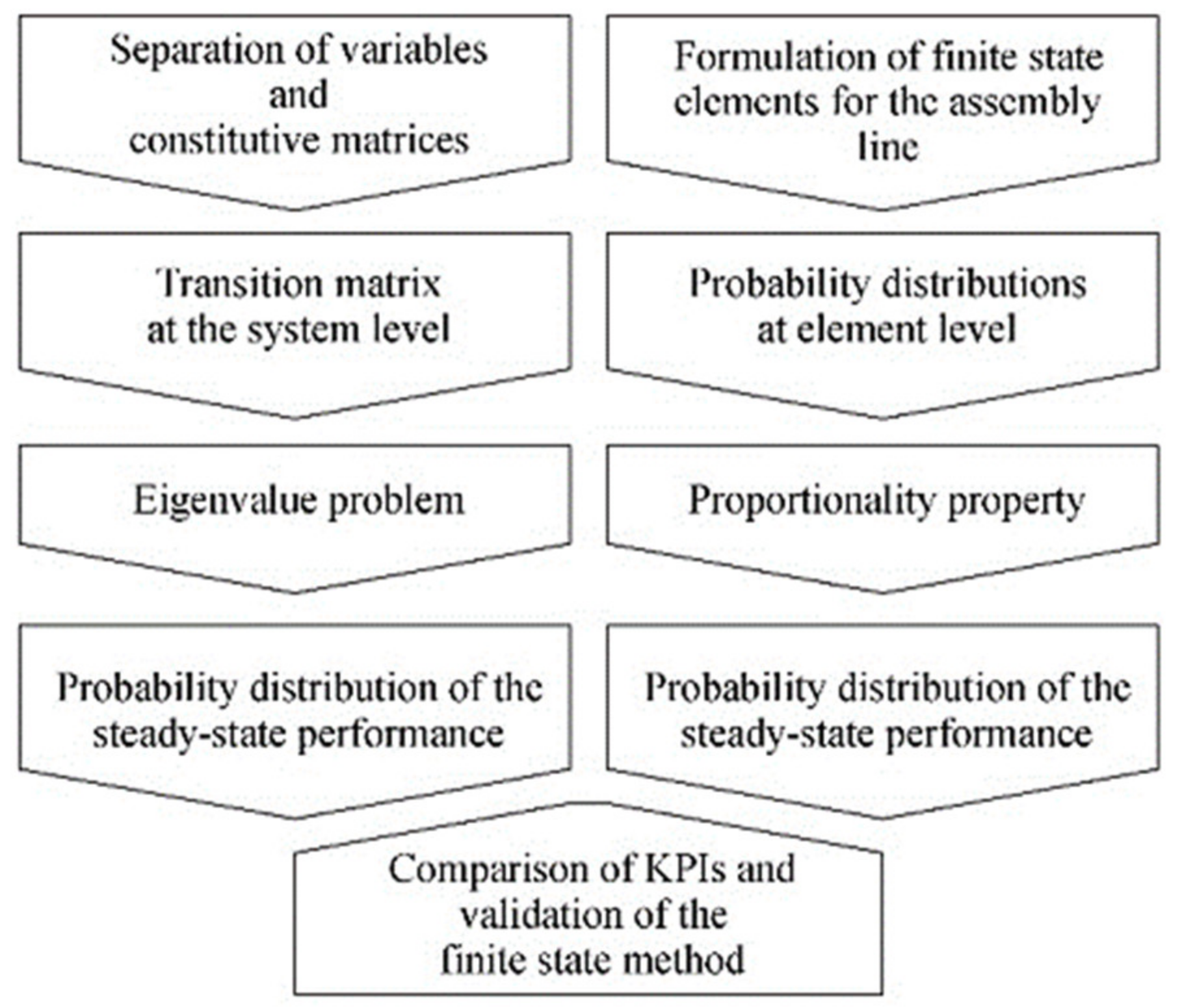
As such, the main contributions of this research paper are (a) the formulation of an analytical solution of the steady-state response of a Bernoulli assembly line in the general case (arbitrary number of machines and buffers of arbitrary capacity) using constitutive transition matrices and the eigenvalue problem; (b) the development, validation, and application of the finite state method while bypassing the system states’ dimensionality issue in the case of the Bernoulli assembly line; and (c) the reconstruction of joint probability distribution while keeping its functional relationships with the system’s properties. This proposition of the joint probability distribution as well as the low computational burden, are of the utmost importance in the evaluation of key performance indicators, improvability considerations, bottleneck identification, and the design of production systems. Additionally, it has to be pointed out that this methodology, involving analytical development and the formulation of the finite state elements, has already been successfully applied in the case of the serial Bernoulli production lines [6,14,42,43] as well as in the case of the Bernoulli splitting lines [3]. In other words, this paper represents a continuation of research that seeks to extend the current application of the Markovian framework in the case of production system engineering.

The remainder of the paper is organized as follows. The analytical formulation of the problem and the formulation of the associated finite state elements are introduced in Section 2. Section 3 presents the application cases including the validation of the FSM and a discussion of the obtained results. The application of the developed theory in the case of the power transformers’ production is summarized in Section 4. Finally, the main conclusions and directions for further research are outlined in Section 5.

2. Mathematical Modeling

Mathematical modeling is performed in two directions (Figure 1). First, the transition matrix in the case of a general assembly line is developed, using the separation of variables and constitutive matrices at the level of each machine. Then, the probability distribution in the case of the steady-state performance is obtained as a solution to the eigenvalue problem. Second, finite state elements are formulated in the case of the assembly line, and the steady-state probability distribution is approximated using the proportionality of distributions at the level of finite state elements. Finally, obtained results are validated through a comparison with the analytical results.

2.1. The Analytical Solution

Consider a Bernoulli assembly line (Figure 2) composed of M machines of the Bernoulli reliability, p_i~Bernoulli(p_i), i = 1, 2, …, M, and M − 1 buffers of capacity N_i ∈ ℕ₀, i = 1, 2, …, M − 1, where machine m_A performs the assembly of parts delivered through R primary flows, and transfers the assembled product for further processing to the secondary flow. Each primary flow is composed of K_i, i = 1, 2, …, R, machines and buffers, while their sum, ${\displaystyle \sum _{i=1}^R{K}_i}$, equals A − 1. This assembly system can be mathematically modeled as an ergodic Markov chain over the system’s state space, composed of all the combinations of the occupancies of buffers [5,44]. However, additional assumptions have to be taken into account, in other words,

• Each machine is in state {up} with probability p_i, conversely it is in state {down} with probability 1 − p_i;
• The state of ith machine does not depend on the state of other machines and is determined at the beginning of each time instance;
• All machines have the same cycle time;
• The system obeys the mass conservation law, thus parts can enter the system only through the first machine at each primary flow, and can exit the only through machine m_M;
• The first machines in the primary flow cannot be starved and machine m_M cannot be blocked.

The steady-state response of a system at-hand can thus be evaluated using the well-known Chapman–Kolmogorov equations, [44,45], relating probabilities P_i and P_j of a system being in the state i, respectively j, in other words,

$$P_i={\displaystyle \sum _{j=1}^S{P}_{ij}{P}_j}, {\displaystyle \sum _{i=1}^S{P}_i}=1$$

(1)

where S is the total number of the system’s states, and P_ij is the transition matrix. In the case when the Markov chain is irreducible and aperiodic, the Chapman–Kolmogorov equation, Equation (1), yields a unique stationary (limiting) solution, in turn reflecting the steady-state response of a stochastic system. One possibility to retrieve this solution is to employ the eigenvalue problem [3,14],

$$\det \left(\left[P\right]-\Lambda \left[I\right]\right)=0,$$

(2)

where [P] is the transition matrix; [I] the unit matrix; and Λ is the eigenvalue. Given the fact that the transition matrix is also stochastic, its first eigenvalue, Λ₁, takes a unit value and is attributed to the first eigenvector {P₁}, representing the normalized form of a stationary solution of the problem. Although this may seem as a quite elegant and straightforward way for the evaluation of the steady-state probability distribution of stochastic systems, it may be far from the truth when realistic systems, composed of large-scale and transition-rich states, are considered. This problem manifests in a 2-fold way, as the inability to formulate the transition matrix and as significant and sometimes unrealistic CPU (central processing unit) resource and time requirements. The former is addressed here in the context of the analytical solution formulation, while the latter is tackled through the formulation of finite state elements.

The formulation of transition probabilities in the general case is a challenging task, particularly when large-scale production systems are considered. The scale of the system, D, is usually determined as the total number of combinations of buffer occupancy levels and equals

$$D={\displaystyle \prod _i^{M-1}\left(N_i+1\right)}$$

(3)

quickly taking quite significant values. For example, in the case when M equals 11 and N_i = 9, the scale of the system, D, takes a value of 10 billion, leading to the conclusion that the dimension of the associated transition matrix equals D², and thus contains 10²⁰ entries. Consequently, a case-by-case formulation of transition matrices is not a reasonable nor advisable strategy. Hence, in this paper, we propose an alternative way to formulate transition matrices by using the concept of the generalized transition matrix formulation.

Each transition matrix, [P], is a function of machine reliabilities, p_i, and thus can be presented as [P] = [P(p₁, p₂, …, p_A, …, p_M)], which upon the separation of its variables can be expressed as a consecutive multiplication of constitutive matrices, [P_i(p_i)], in other words,

$$\begin{array}{l}\left[P\left(p_1,p_2,\dots ,p_A,\dots p_M\right)\right]=\\ \hspace{1em}\hspace{1em} \left[P_1\left(p_1\right)\right]\left[P_2\left(p_2\right)\right]\dots \left[P_A\left(p_A\right)\right]\dots \left[P_M\left(p_M\right)\right]={\displaystyle \prod _i^M\left[P_i\left(p_i\right)\right]}.\end{array}$$

(4)

The ith constitutive matrix, [P_i(p_i)], reflects the contribution of machine m_i to the movement of the stochastic system from state $〈H^n〉=〈h_1^n,h_2^n\dots ,h_A^n,\dots h_{M-1}^n〉$ in the nth cycle, where $h_i^n$, i = 1, 2, …, M − 1 is the state of the ith buffer in the nth cycle, to state $〈H^{n+1}〉=〈h_1^{n+1},h_2^{n+1}\dots ,h_A^{n+1},\dots h_{M-1}^{n+1}〉$, attributed to the cycle n + 1. In the considered case of the assembly production line, four different types of constitutive matrices can be formulated (i.e., $\left[P_{\zeta }\right]$, $\left[P_{\overline{\zeta }}\right]$, $\left[P_A\right]$, and $\left[P_M\right]$), where ζ = {1, K₁ + 1, K₁ + K₂ + 1, …, A − K_R} and $\overline{\zeta }$ = {1, 2, …, M − 1}\{ζ, A}.

The generic structure of each constitutive matrix contains four different entries, namely 1 − p_i in the case when the ith machine does not alter the state of the system due to a breakdown, p_i, when the state of the system is altered due to the activity of machine m_i, 1 in the case when the state of the system cannot be altered due to starvation or blockage of machine m_i, and 0 for all other cases. Therefore, the constitutive matrix $\left[P_{\zeta }\right]$ is equal to

$$\left[P_{\zeta }\right]=\left\{\begin{array}{l}1-p_{\zeta }, \mathrm{if} h_{\psi }^{n+1}=h_{\psi }^n,h_{\zeta }^n<N_{\zeta }\\ p_{\zeta }, \mathrm{if} h_{\zeta }^{n+1}=h_{\zeta }^n+1,h_{\overline{\psi }}^{n+1}=h_{\overline{\psi }}^n,h_{\zeta }^n<N_{\zeta }\\ 1, \mathrm{if} h_{\psi }^{n+1}=h_{\psi }^n,h_{\zeta }^n=N_{\zeta }\\ 0, \mathrm{else},\end{array}\right.$$

(5)

where $\psi =\left\{1,2,3,\dots ,M-1\right\}$ and $\overline{\psi }=\psi \backslash \zeta$. Similarly, it follows that the second constitutive matrix, $\left[P_{\overline{\zeta }}\right]$, can be formulated as

$$\left[P_{\overline{\zeta }}\right]=\left\{\begin{array}{l}1-p_{\overline{\zeta }}, \mathrm{if} h_{\psi }^{n+1}=h_{\psi }^n,h_{\overline{\zeta }-1}^n>0,h_{\overline{\zeta }}^n<N_{\overline{\zeta }}\\ p_{\overline{\zeta }}, \mathrm{if} h_{\overline{\zeta }-1}^{n+1}=h_{\overline{\zeta }-1}^n-1,h_{\overline{\zeta }}^{n+1}=h_{\overline{\zeta }}^n+1,h_{\overline{\psi }}^{n+1}=h_{\overline{\psi }}^n,h_{\overline{\zeta }-1}^n>0,h_{\overline{\zeta }}^n<N_{\overline{\zeta }}\\ 1, \mathrm{if} h_{\psi }^{n+1}=h_{\psi }^n,h_{\overline{\zeta }-1}^n=0\vee h_{\overline{\zeta }}^n=N_{\overline{\zeta }}\\ 0, \mathrm{else},\end{array}\right.$$

(6)

where $\overline{\psi }=\psi \backslash \overline{\zeta }$. The third constitutive matrix is associated with the machine performing assembly operations and is equal to

$$\left[P_A\right]=\left\{\begin{array}{l}1-p_A, \mathrm{if} h_{\psi }^{n+1}=h_{\psi }^n,h_{\xi }^n>0,h_A^n<N_A\\ p_A, \mathrm{if} h_{\xi }^{n+1}=h_{\xi }^n-1,h_A^{n+1}=h_A^n+1,h_{\overline{\psi }}^{n+1}=h_{\overline{\psi }}^n,h_{\xi }^n>0,h_A^n<N_A\\ 1, \mathrm{if} h_{\psi }^{n+1}=h_{\psi }^n,h_{\xi }^n=0\vee h_A^n=N_A\\ 0, \mathrm{else},\end{array}\right.$$

(7)

where $\xi =\left\{K_1,K_1+K_2,K_1+K_2+K_3,\dots ,A-1\right\}$ is a set of buffers placed immediately before the assembly machine, m_A, and $\overline{\psi }=\psi \backslash \xi$. Finally, the constitutive matrix, associated with machine m_M, $\left[P_M\right]$, equals

$$\left[P_M\right]=\left\{\begin{array}{l}1-p_M, \mathrm{if} h_{\psi }^{n+1}=h_{\psi }^n,h_{M-1}^n>0\\ p_M, \mathrm{if} h_{M-1}^{n+1}=h_{M-1}^n-1,h_{\overline{\psi }}^{n+1}=h_{\overline{\psi }}^n,h_{M-1}^n>0\\ 1, \mathrm{if} h_{\psi }^{n+1}=h_{\psi }^n,h_{M-1}^n=0\\ 0, \mathrm{else},\end{array}\right.$$

(8)

where $\overline{\psi }=\psi \backslash \left(M-1\right)$. The procedure for the transition matrix formulation is illustrated in Appendix A in the simple case of an assembly system composed of three machines and two buffers of capacity N₁ = N₂ = 2, while more complex cases are taken into account in Section 3.

2.2. The Finite State Method

The analytical solution of the assembly systems’ steady-state response reveals the complexity of the problem, particularly as the formulation of the transition matrix becomes rather cumbersome and impractical, even for the simplest cases, not to mention the issues of the consecutive multiplication of large-scale matrices and the solution of the eigenvalue problem. Therefore, a more convenient way to evaluate performance measures of the assembly systems, especially when design issues are in question, is to consider some of the approximative procedures, for example, the finite state method. This method has already been successfully applied in the case of Bernoulli serial and splitting lines [3,6], and will thus be further extended here in the case of assembly systems.

The central idea of the finite state method is to model complex transition relationships of an assembly system in the general case by using the simple and analytical solution of the two-machine-one buffer problem. In this way, an intricate mathematical problem can be significantly simplified, while keeping all of the necessary relationships between the system properties and key performance indicators. The analytical solution of the two machine-one buffer problem can be retrieved in several ways, however, its formulation, using a recursive procedure, is readily available in the literature [5], and equals

$$P_0=\frac{\left(1-p_L\right)\left(1-\alpha \right)}{1-\frac{p_L}{p_R}{\alpha }^N}, P_i=\frac{{\alpha }^i}{1-p_R}{P}_0, i=1,2,\dots ,N, \alpha =\frac{p_L\left(1-p_R\right)}{p_R\left(1-p_L\right)},$$

(9)

where P_i, i = 0, 1, 2, …, N, is the probability of a system being in state I; N is the capacity of the buffer; and p_L and p_R are the reliabilities of machines positioned, respectively, at the left and right hand of the buffer. The same solution can be applied when formulating finite state elements of the assembly production line concerning the weakest machine, m_m, where m is such that

$$p_m=\min \left\{p_1,p_2,\dots ,p_M\right\}$$

(10)

An example of the structural scheme of finite state elements is presented in Figure 3 including the primary flows and a secondary flow. In this case, the total number of M − 1 elements can be formulated, with each composed of only two machines and one buffer placed between them. Depending on the relative position of machine m_m, finite state elements can be formulated and characterized as upstream or downstream.

In the case when m ≤ K₁, machine m_m is placed in the first primary flow (r = 1), while it is placed in the second primary flow (r = 2) when K₁ < m ≤ K₁ + K₂. In the more general case, machine m_m is a component of the r^th primary flow if m falls within range $〈\left.{\displaystyle \sum _{i=1}^{K_{r-1}}i},{\displaystyle \sum _{i=1}^{K_r}i}\right]$, r = 2, 3, …, R. In a special case when r = 1, this range is simplified to the form $〈\left.1,{\displaystyle \sum _{i=1}^{K_1}i}\right]$. Additionally, when m ≥ A, machine m_m is placed in the secondary flow. Consequently, the assembly system (Figure 3) can be decomposed into a set of serial lines while extending flows not containing the weakest machine with the additional (imaginary) machine to the right in the case of primary flows and to the left in the case of the secondary flow. This fictive machine is presented in Figure 3b using a dashed line. Thus, upstream elements are defined in the range $e=\left[1,m-1\right]$ and $e=\left[K_1,K_1+K_2-1\right]$. Similarly, downstream elements range within $e=\left[m,K_1\right]$ and $e=\left[A-1,M-1\right]$.

In the case of the upstream elements, the left-hand side machine is associated with a reliability of p_L = p_e, $e=\left[1,m-1\right]$ and $e=\left[K_1,K_1+K_2-1\right]$, while the reliability of the right-hand side machine always equals p_R = p_m. Consequently, the steady-state distribution at upstream element level, $P^{\left(e\right)}$, equals

$$\left\{P^{\left(e\right)}\right\}=\left\{\begin{array}{l}\frac{\left(1-p_e\right)\left(1-\alpha \right)}{1-\frac{p_e}{p_m}{\alpha }^N}\\ P_1=\frac{{\alpha }^i}{1-p_m}{P}_0\\ \dots \\ P_{N_e}=\frac{{\alpha }^{N_e}}{1-p_m}{P}_0\end{array}\right\}, \alpha =\frac{p_e\left(1-p_m\right)}{p_m\left(1-p_e\right)},$$

(11)

where N_e is the capacity of the buffer associated with element e. Similarly, the steady-state distribution of downstream elements, when the reliability of the left-hand side machine equals p_L = p_m, and the reliability of the right-hand side machine p_R = p_e, $e=\left[m,K_1\right]$ and $e=\left[A-1,M-1\right]$ equals

$$\left\{P^{\left(e\right)}\right\}=\left\{\begin{array}{l}\frac{\left(1-p_m\right)\left(1-\alpha \right)}{1-\frac{p_m}{p_e}{\alpha }^N}\\ P_1=\frac{{\alpha }^i}{1-p_e}{P}_0\\ \dots \\ P_{N_e}=\frac{{\alpha }^{N_e}}{1-p_e}{P}_0\end{array}\right\}, \alpha =\frac{p_m\left(1-p_e\right)}{p_e\left(1-p_m\right)}.$$

(12)

Once steady-state distributions at the level of finite state elements are defined, the global, or system level distribution can be derived, assuming the independence of events on each buffer. Consequently, the probability of an assembly system being in state $〈H〉=〈h_1,h_2,\dots h_{M-1}〉$, $P_{h_1{h}_2\dots h_{M-1}}$, is equal to an intersection of events $\left\{h_1\right\}$, $\left\{h_2\right\}$, …, $\left\{h_{M-1}\right\}$,

$$P_{h_1{h}_2\dots h_{M-1}}=P\left[{\displaystyle \underset{i=1}{\overset{M-1}{\cap }}\left\{h_i\right\}}\right]={\displaystyle \prod _{e=1}^{M-1}{P}_{i=h_e}^{\left(e\right)}}$$

(13)

where $P_{i=h_e}^{\left(e\right)}$ is the probability of the eth buffer being in state i.

2.3. Performance Measures

Once steady-state distribution at the system level is formulated, it is possible to evaluate associated performance measures such as the production rate (PR), work-in-process at the i^th buffer (WIP_i), probabilities of blockage (BL), and probabilities of starvations (ST). The definitions of the production rate and work-in-process in the case of an assembly system remain the same as in the case of a typical Bernoulli serial line. On the other hand, defining the probabilities of blockage and starvation requires some modifications in the case of machines m_ξ (recalling that $\xi =\left\{K_1,K_1+K_2,K_1+K_2+K_3,\dots ,A-1\right\}$) and m_A due to the structure of the assembly lines. Hence, the formulation of the production rate and work-in-process will be omitted here as it is well-known and available in the literature (e.g., [3,5,14]).

The probability of the blockage of machine m_ξ can be formulated as the union of events [{m_ξ is up}∩{b_ξ is full}∩{m_A is down}], [{m_ξ is up}∩{b_ξ is full}∩{m_A is blocked}], and [{m_ξ is up}∩{b_ξ is full}∩{m_A is starved}], yielding

$$B{L}_{\xi }=p_{\xi }\left(1-p_A+B{L}_A+S{T}_A^{\prime }\right){\displaystyle \sum _{h_1= 0}^{N_1}{\displaystyle \sum _{h_2= 0}^{N_2}\dots }{\displaystyle \sum _{h_{M-1}}^{N_{M-1}}{P}_{h_1{h}_2\dots h_{\xi }=N_{\xi }\dots h_{M-1}}}},$$

(14)

where BL_A is the probability of blockage of machine m_A. The probability $S{T}_A^{\prime }$ takes into account the starvation of machine m_A due to the emptiness of buffers b_ξ, other than a considered machine, in other words,

$$S{T}_A^{\prime }=S{T}_A-{\displaystyle \sum _{h_1= 0}^{N_1}{\displaystyle \sum _{h_2= 0}^{N_2}\dots }{\displaystyle \sum _{h_{M-1}}^{N_{M-1}}{P}_{h_1{h}_2\dots h_{\xi }= 0\dots h_{M-1}}}},$$

(15)

where ST_A is the probability of the starvation of machine m_A, determined as a union of events [{one buffer from the set ξ is empty}∩{m_A is up}], [{two buffers from the set ξ are empty}∩{m_A is up}], …, [{R buffers from the set ξ are empty}∩{m_A is up}], or as

$$\begin{array}{l}S{T}_A=p_A\left({\displaystyle \sum _{h_1= 0}^{N_1}{\displaystyle \sum _{h_2= 0}^{N_2}\dots }{\displaystyle \sum _{h_{M-1}}^{N_{M-1}}{P}_{\dots h_{K_1}= 0\dots }}}+{\displaystyle \sum _{h_1= 0}^{N_1}{\displaystyle \sum _{h_2= 0}^{N_2}\dots }{\displaystyle \sum _{h_{M-1}}^{N_{M-1}}{P}_{\dots h_{K_1}= 0\dots h_{K_2}= 0\dots }}}+\dots \right.\\ \left.\hspace{1em}\hspace{1em}\hspace{1em}\hspace{1em}\hspace{1em}\hspace{1em}\hspace{1em}\hspace{1em}\hspace{1em}\hspace{1em}\hspace{1em}\hspace{1em}\hspace{1em}\hspace{1em}\hspace{1em}\hspace{1em}\hspace{1em}\hspace{1em}\hspace{1em}\hspace{1em}+{\displaystyle \sum _{h_1= 0}^{N_1}{\displaystyle \sum _{h_2=0}^{N_2}\dots }{\displaystyle \sum _{h_{M-1}}^{N_{M-1}}{P}_{\dots h_{\xi }= 0\dots }}}\right).\end{array}$$

(16)

3. Application of the Developed Theory

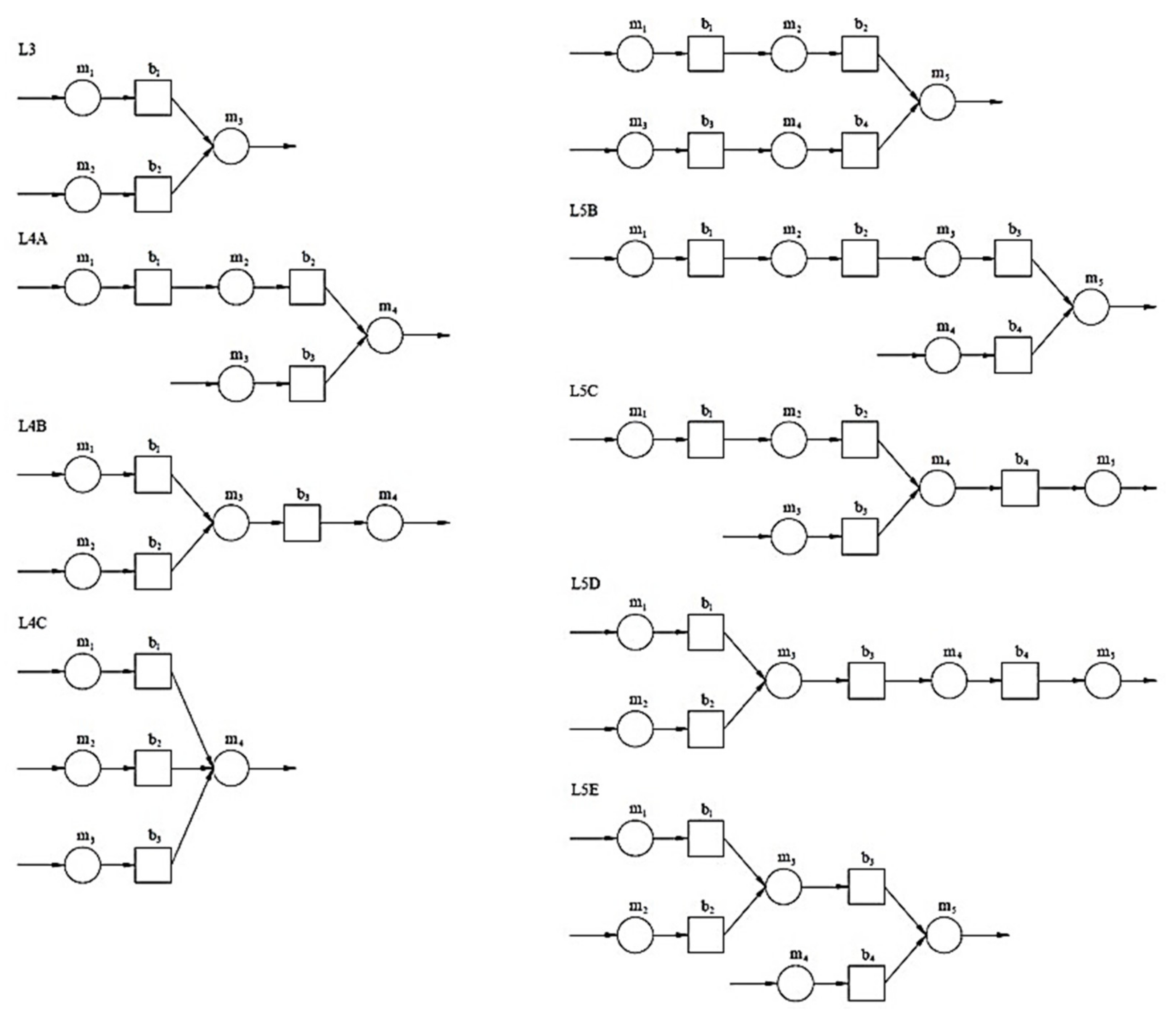
The presented theoretical framework has been applied in several cases including theoretical assembly lines composed of three, four, and five machines, in different arrangements (Figure 4). The respective machine reliabilities as well as the even and uneven distributions of buffer capacities, are summarized in

Table 1. Machine reliabilities and the capacities of buffers in the case of theoretical assembly lines.

Line	p1	p2	p3	p4	p5	N1	N2	N3	N4
L3	0.4	0.5	0.6	/	/	N	N	/	/
	0.4	0.5	0.6	/	/	N	½N	/	/
L4A	0.4	0.5	0.6	0.7	/	N	N	N	/
	0.4	0.5	0.6	0.7	/	N	⅔N	⅓N	/
L4B	0.4	0.5	0.6	0.7	/	N	N	N	/
	0.4	0.5	0.6	0.7	/	N	⅔N	⅓N	/
L4C	0.4	0.5	0.6	0.7	/	N	N	N	/
	0.4	0.5	0.6	0.7	/	N	⅔N	⅓N	/
L5A	0.4	0.5	0.6	0.7	0.8	N	N	N	N
	0.4	0.5	0.6	0.7	0.8	N	¾N	½N	¼N
L5B	0.4	0.5	0.6	0.7	0.8	N	N	N	N
	0.4	0.5	0.6	0.7	0.8	N	¾N	½N	¼N
L5C	0.4	0.5	0.6	0.7	0.8	N	N	N	N
	0.4	0.5	0.6	0.7	0.8	N	¾N	½N	¼N
L5D	0.4	0.5	0.6	0.7	0.8	N	N	N	N
	0.4	0.5	0.6	0.7	0.8	N	¾N	½N	¼N
L5E	0.4	0.5	0.6	0.7	0.8	N	N	N	N
	0.4	0.5	0.6	0.7	0.8	N	¾N	½N	¼N

.

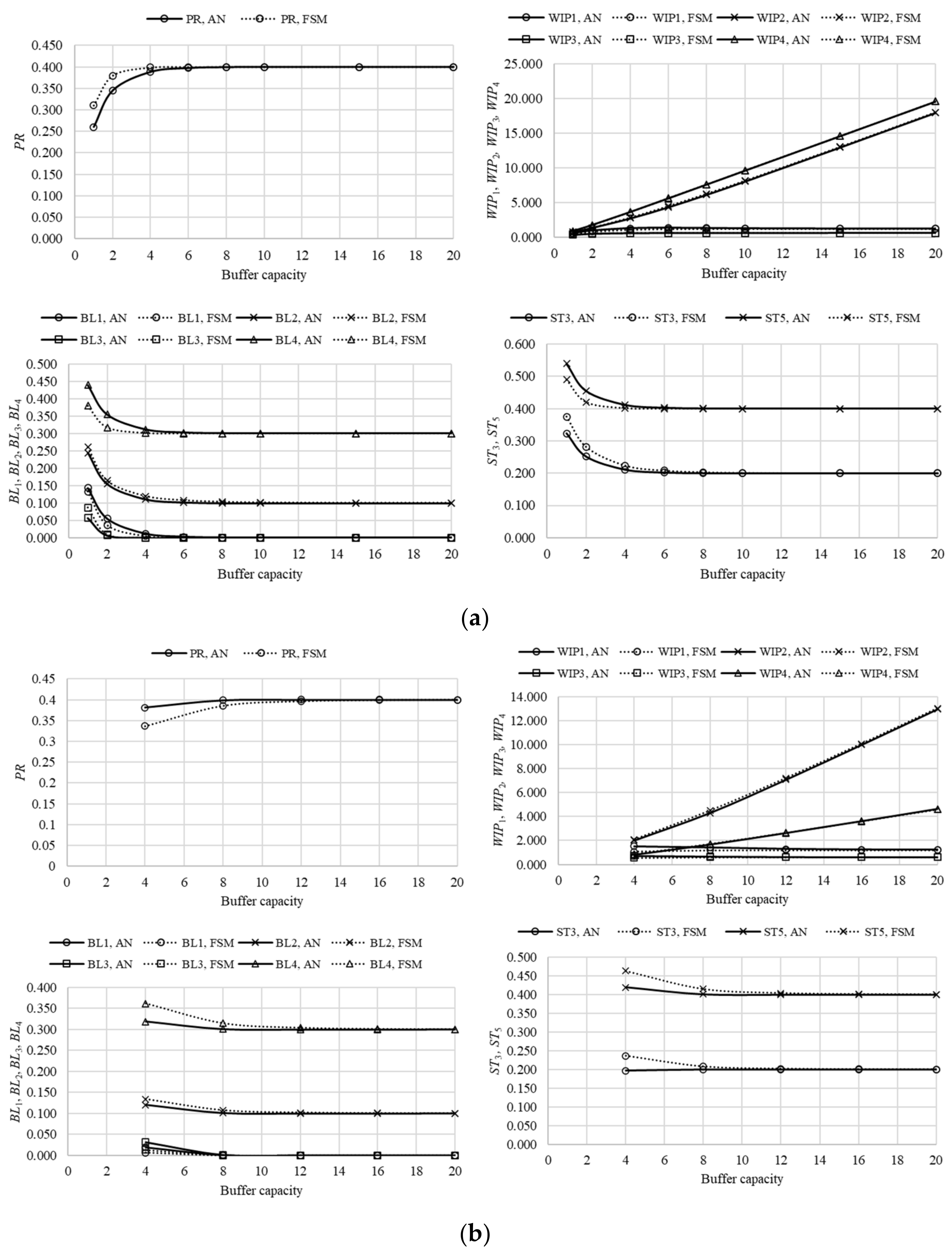
The range of buffer capacities was considered between 1 and 20 per buffer (21 in the case of lines with four machines). Each case was evaluated using the analytical approach (AN) and the finite state method (FSM) to enable their comparison and validation. Hence, in the first case, key performance indicators, namely the production rate (PR), the work-in-process at the ith buffer (WIP_i), and the probabilities of blockage and starvation of machines (BL_i and ST_i) were evaluated using steady-state probability distribution, obtained using Equations (2)–(8), while the same performance indicators were obtained in the second case, using the distribution retrieved by the finite state method, Equations (11)–(13). The obtained results are presented in Figure 5, Figure 6, Figure 7, Figure 8, Figure 9, Figure 10, Figure 11, Figure 12 and Figure 13 including even and uneven buffer capacities in each of the considered assembly systems.

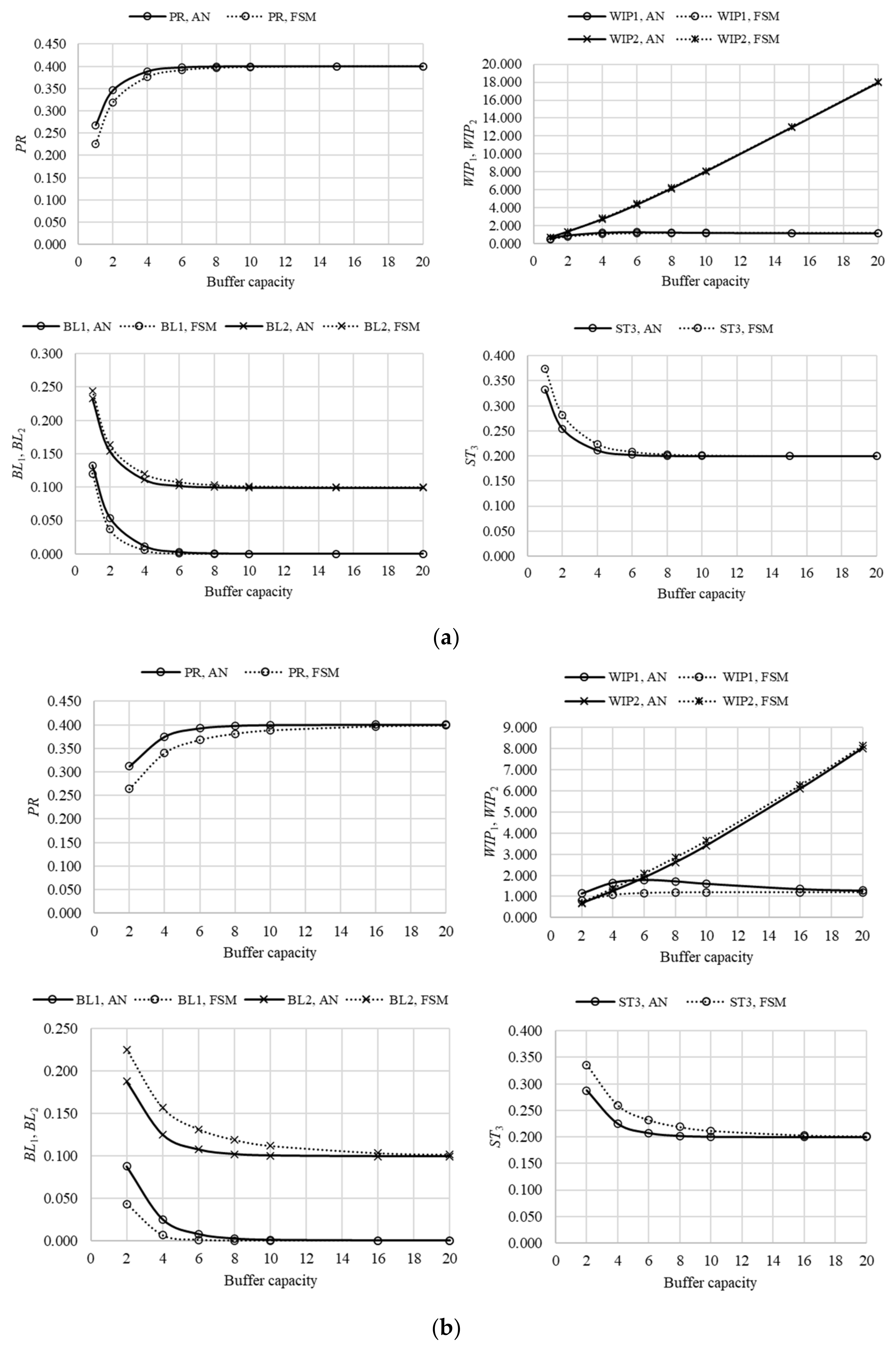
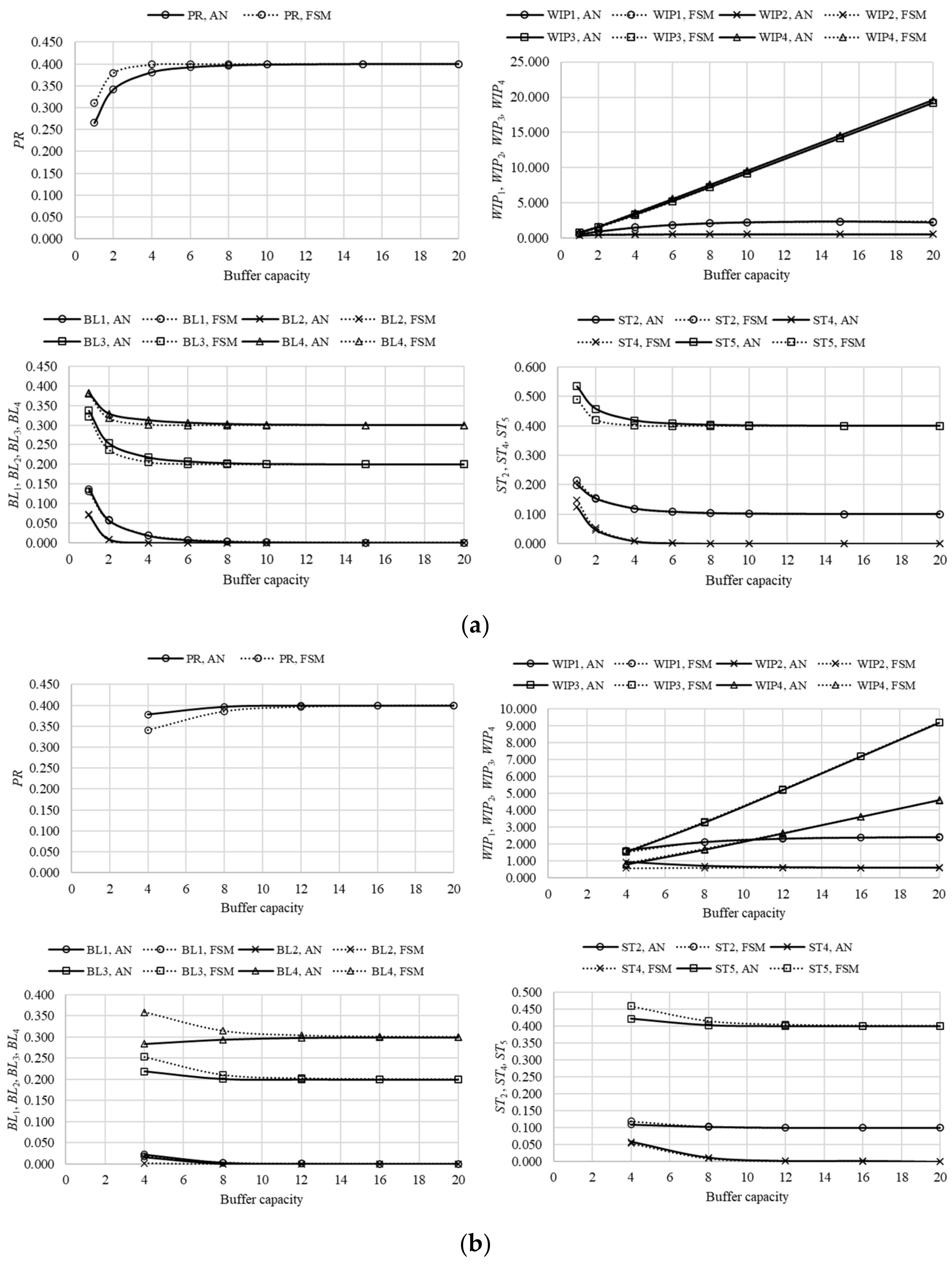
The performance measures of the simplest assembly system, composed of three machines and two buffers (line L3), are presented in Figure 5, where agreement between the results, obtained using different approaches, can be seen. Although, the finite state method demonstrates some discrepancies concerning the analytical approach, in the case of uneven distribution and lower range of buffer capacities. Even though these discrepancies are more pronounced when compared to, for example, Bernoulli serial or splitting lines [3,14]), they diminish quickly as the capacity of the buffers increases. The asymptotic values of the performance measures retain the same properties as in the case of Bernoulli serial and splitting lines. Thus, the production rate of line L3 approaches the reliability of the worst machine in the system, which is $\underset{N\to \infty }{PR}=\min \left(p_i\right)$. Similarly, the work-in-process increases almost linearly when the machine of lower reliability induces a blockage of the machine placed immediately before the respective buffer. Alternatively, the work-in-process quickly converges to a finite limit. The probability of blockage BL₁ diminishes quickly as the reliability of machine m₃≡m_A is greater than the reliability of machine m₁, while BL₂ converges to the difference p₂-p_m, where p_m = p₁. Similarly, the probability of starvation ST3 approaches the value p₃-p_m, with an increase in buffer capacity.

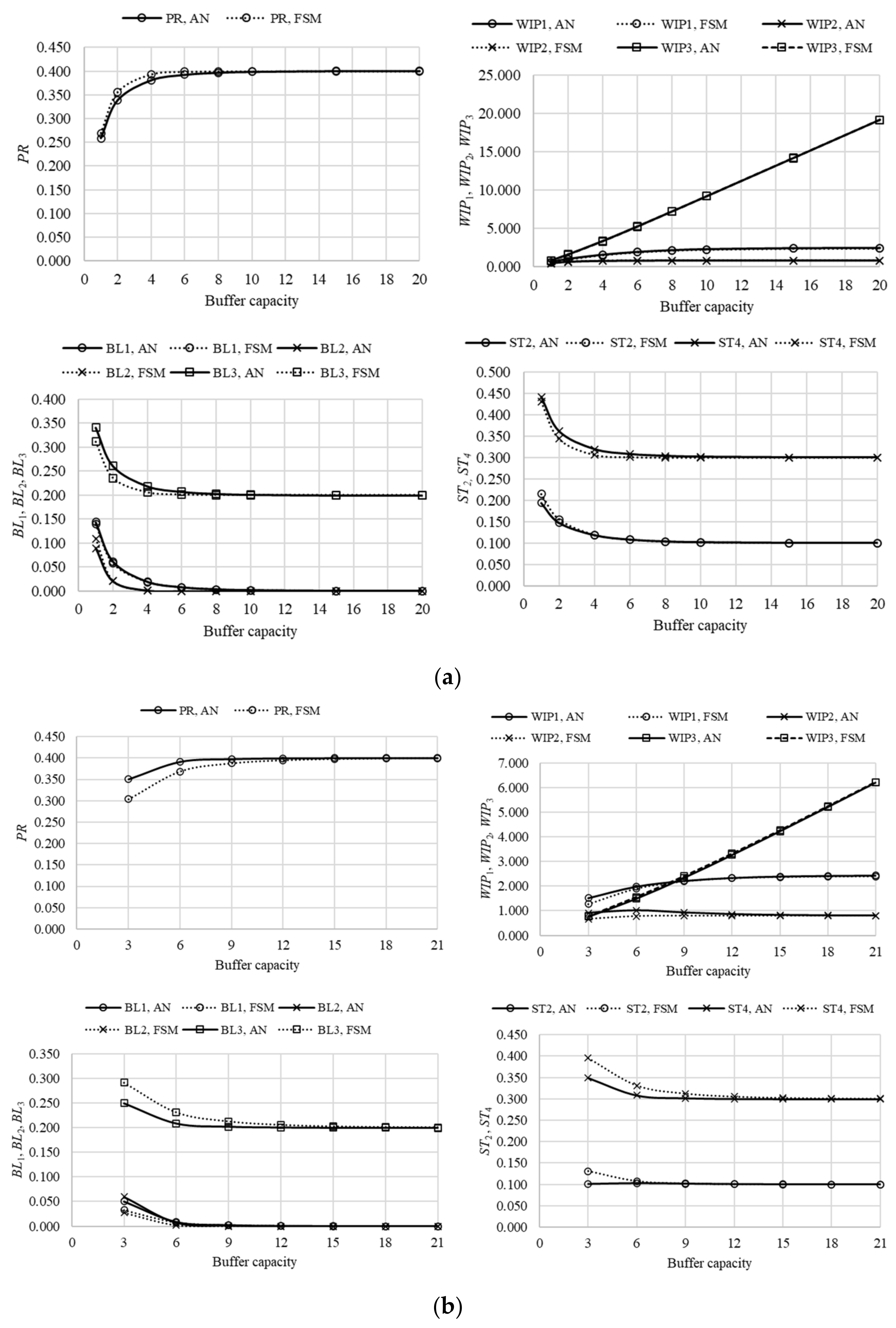
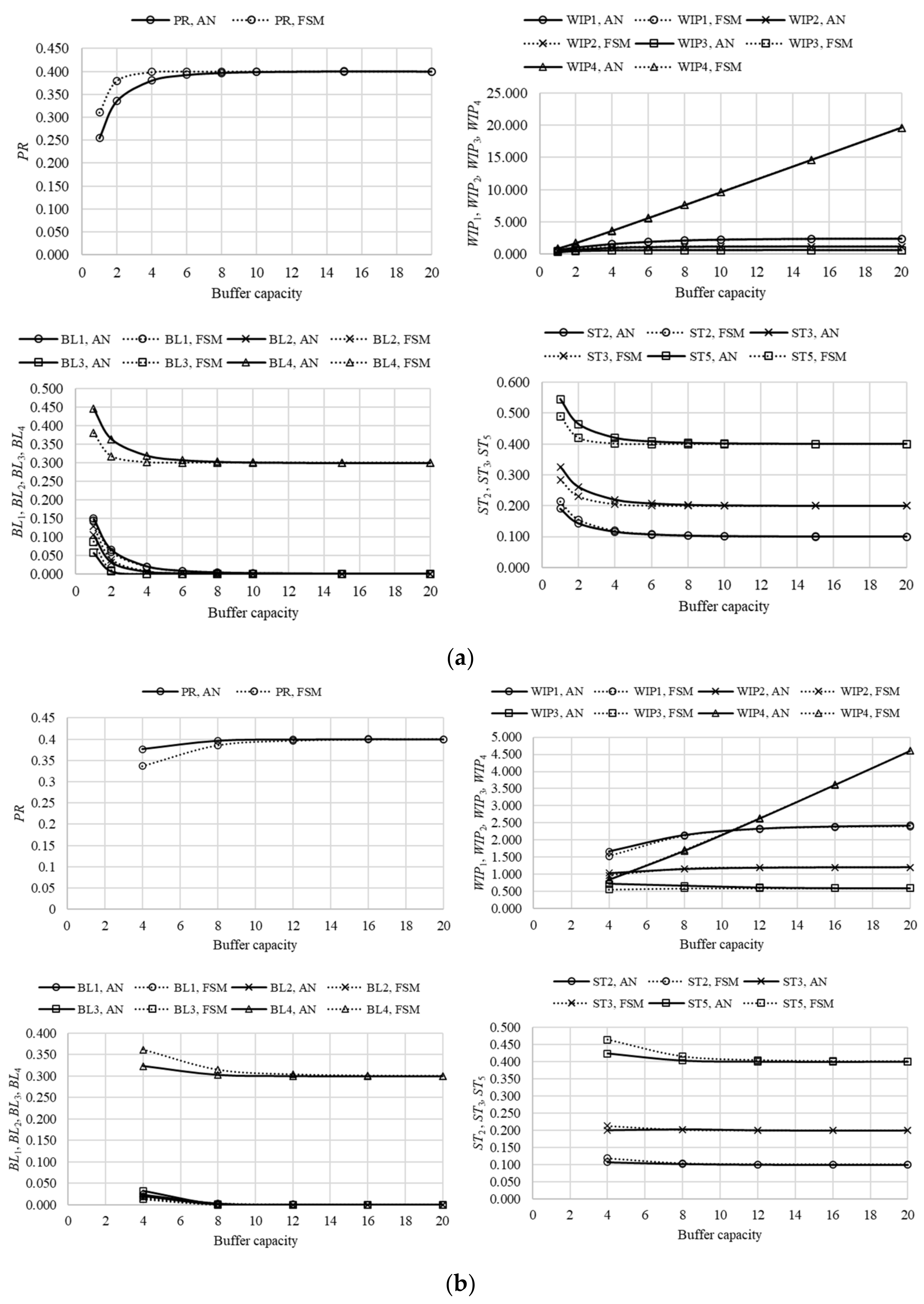
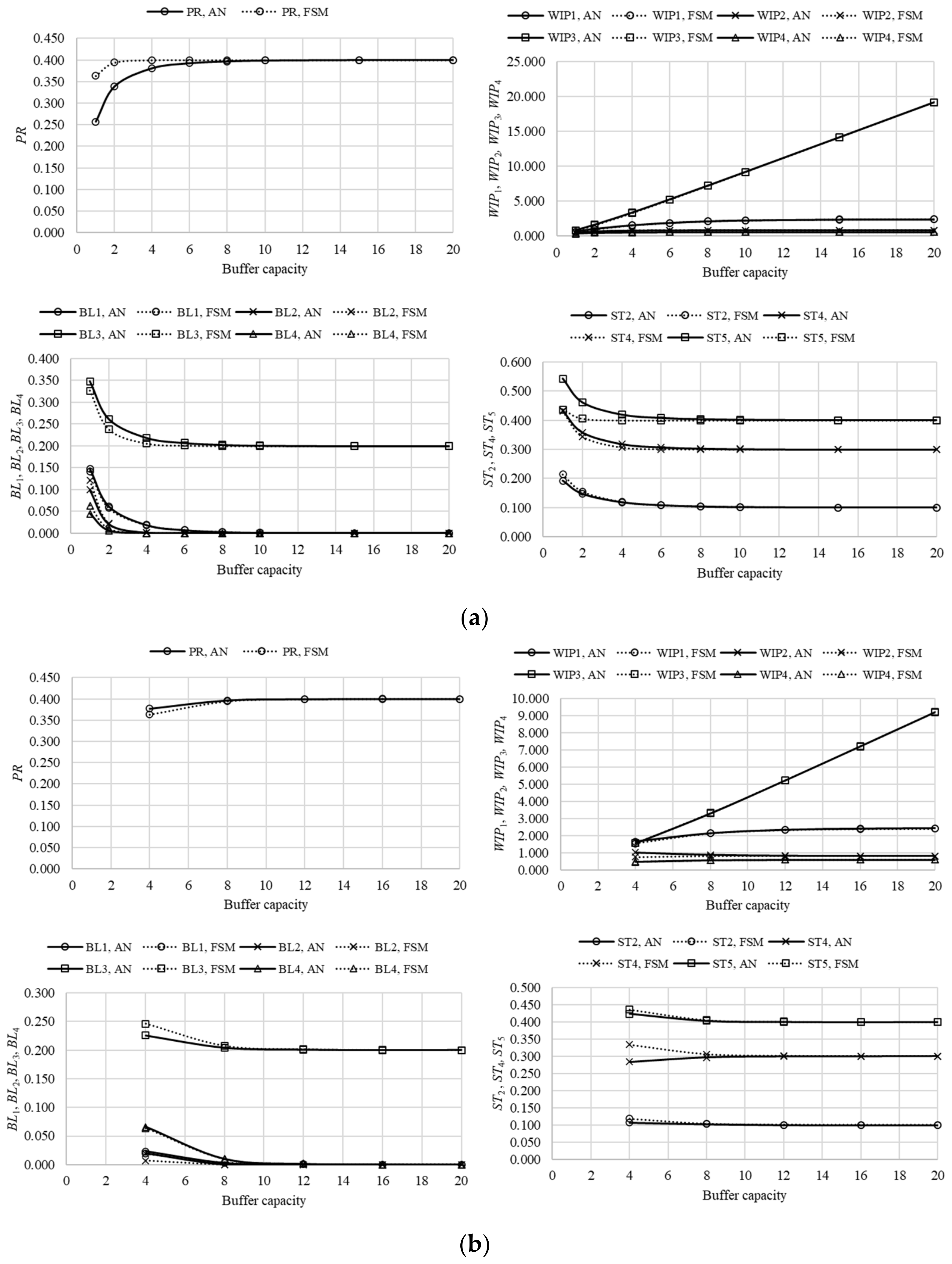
The comparison of results obtained in the case of assembly systems, composed of four machines and three buffers in different arrangements, is presented in Figure 6, Figure 7 and Figure 8 (lines L4A, L4B, and L4C, respectively). Slight discrepancies between the results of the analytical evaluation and evaluation using the finite state method can be noted, similar to the case of line L3. However, these discrepancies were pronounced to a lesser extent as the systems’ states included a greater number of possibilities, thus enabling the finite state method to discretize state spaces more efficiently. As in the previous case, the performance measures approached asymptotic values quickly, while WIP₃ grew linearly with the increase in the buffer capacity. The asymptotic values retained the same logic and were equal to p_m in the case of the production rate, p_i-p_m in the case of the probability of blockage (when induced by a subsequent and less reliable machine, otherwise it equals 0), and p_i-p_m in the case of the probability of starvation.

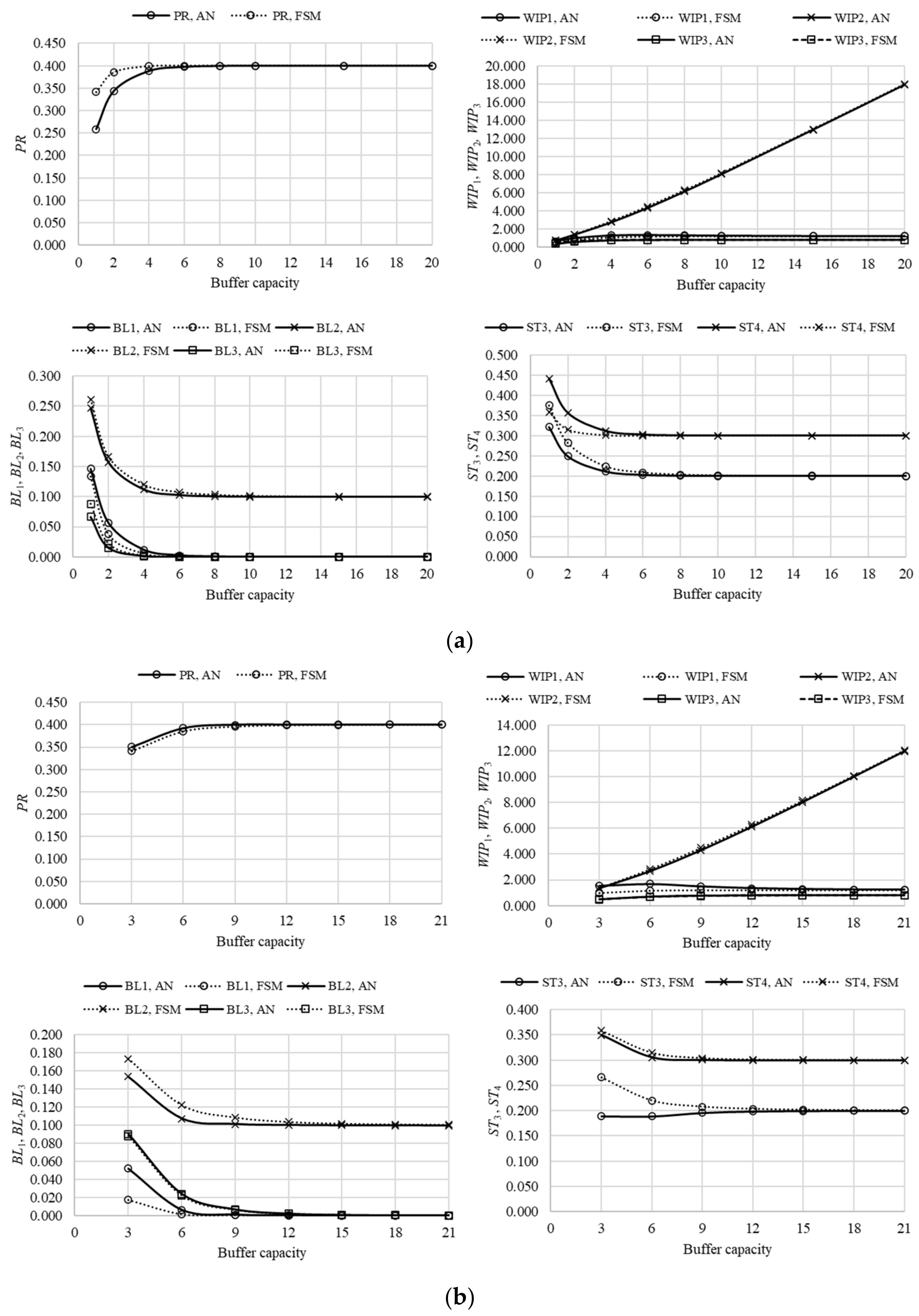
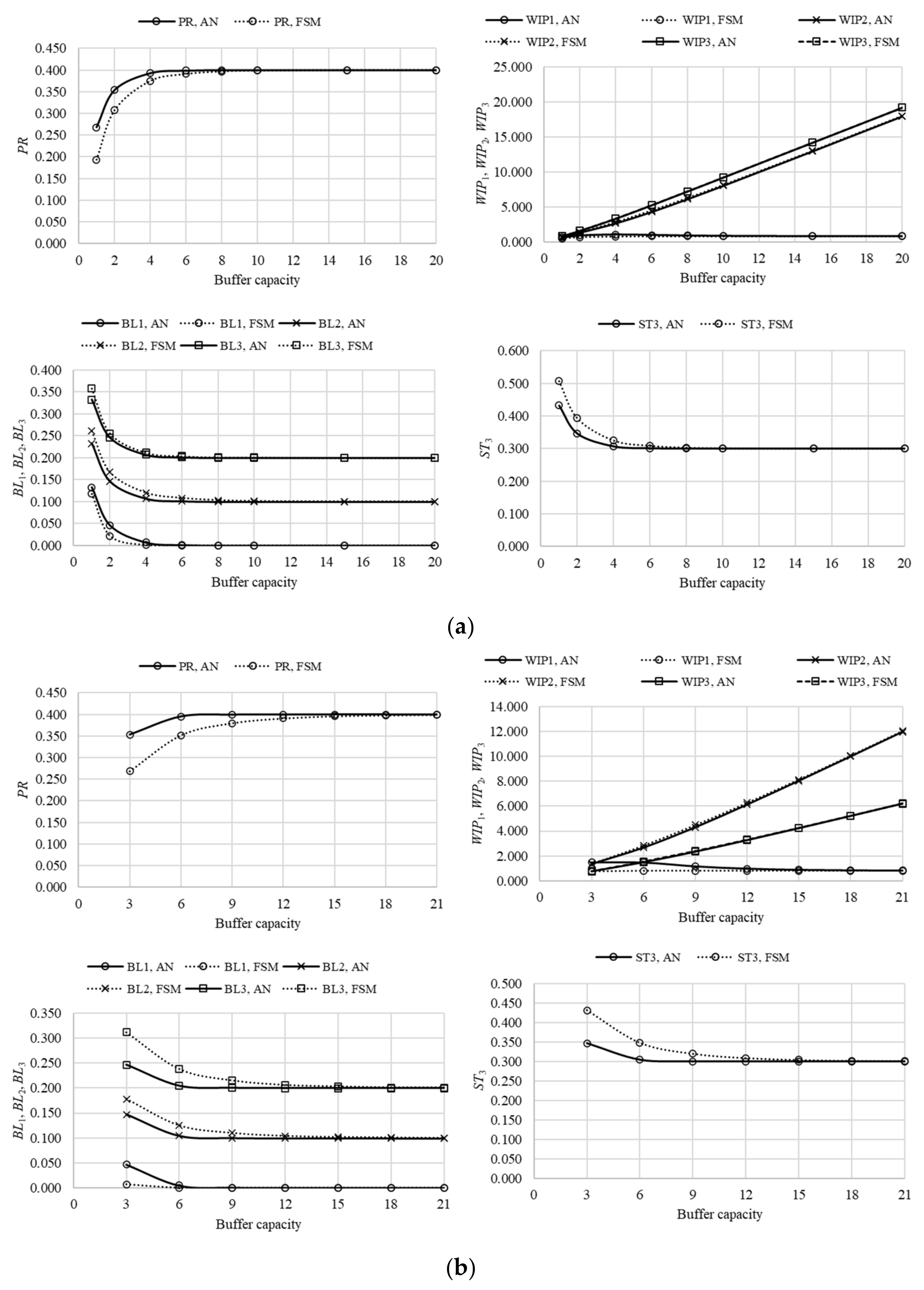
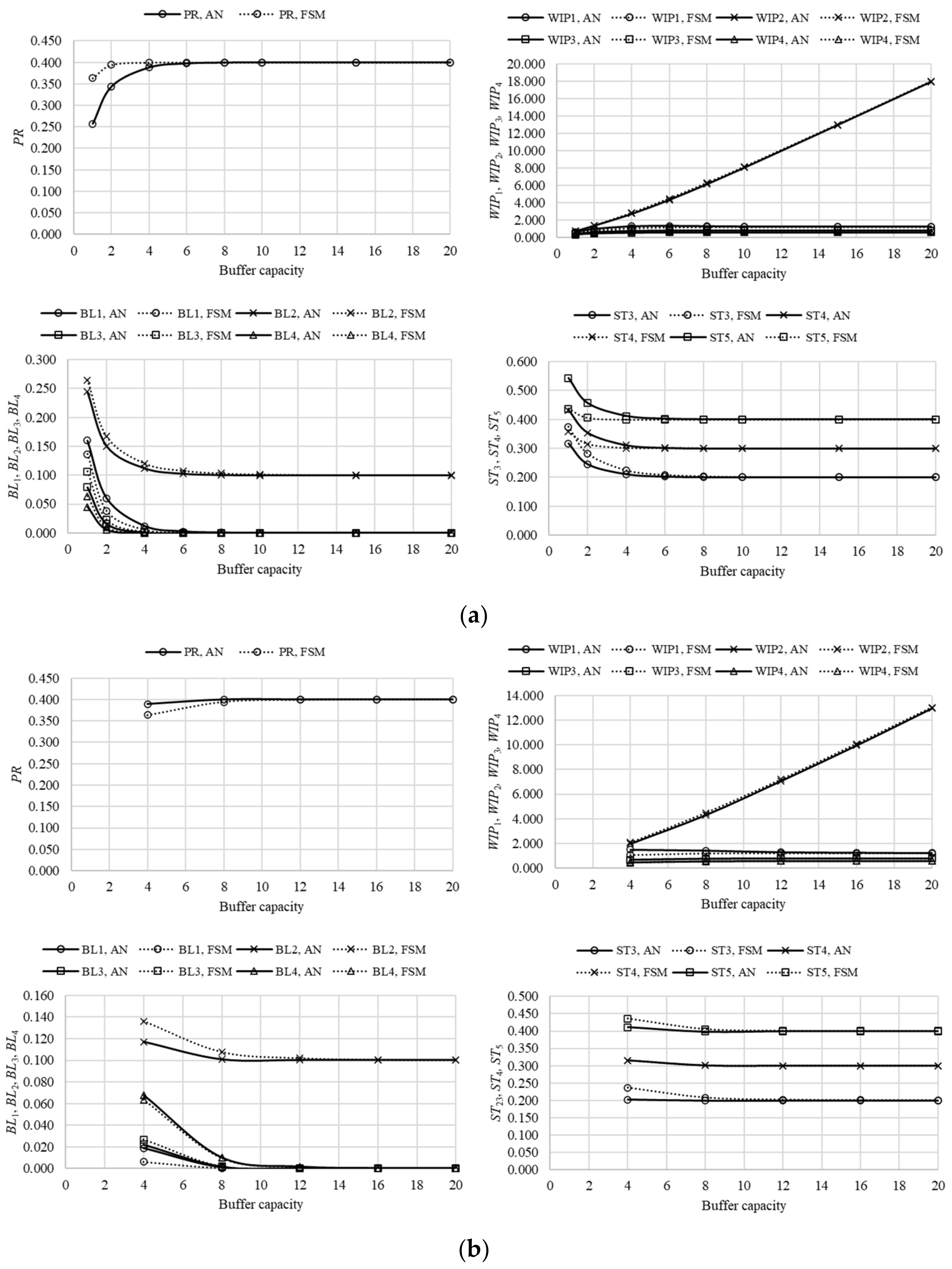
The performance measures of assembly systems composed of five machines and four buffers in different arrangements, systems L5A–L5E, are presented in Figure 9, Figure 10, Figure 11, Figure 12 and Figure 13. The comparison of results, obtained using the finite state method against respective data, determined using the analytical approach, again revealed that the proposed approximative method yielded quite reliable results, with a tendency of an accuracy increase as the system becomes more complex. The asymptotic properties of the performance measures, determined in the case of systems L5A–L5E, remained the same as in the case of line L3 and lines L4A–L4C. That is, the production rate always converged with the reliability of the worst machine in the system, while the probability of starvation asymptotically approached the difference between the reliability of the respective and the worst machine, p_i-p_m. The work-in-process demonstrated a 2-fold character. In the case when a subsequent machine is less reliable, when compared to its antecedent counterpart, work-in-process grows linearly with an increase in buffering capacity. Alternatively, it quickly takes a constant value (i.e., it is not affected by an increase in buffering capacity). Finally, the probability of blockage may take two different asymptotic characters. In the case when a subsequent machine is more reliable, when compared to the respective one, it will take zero value. Alternatively, it will amount to p_i-p_m.

3.1. Discussion

Based on the compared performance measures, it may be noted that FSM approximately yields the same results as the analytical approach regardless of line arrangement. That is, the accuracy of the approximation is not affected by the relative positions of the machines. This conclusion is of great significance, as it supports the extension of the approach to more complex and realistic cases of assembly systems including multiple assembly machines and secondary flows.

An absolute error of the results obtained using FSM concerning the analytical solution is presented in

Table 2. An absolute error of the results obtained using FSM concerning the analytical solution.

M	N	D	EPR	EWIP1	EWIP2	EWIP3	EWIP4	EBL1	EBL2	EBL3	EBL4	EST2	EST3	EST4
3	1	4	0.042	0.073	0.018	/	/	0.012	0.012	/	/	/	0.042	/
	2	9	0.027	0.146	0.012	/	/	0.017	0.009	/	/	/	0.027	/
	4	25	0.012	0.196	0.111	/	/	0.006	0.008	/	/	/	0.012	/
	6	49	0.006	0.158	0.152	/	/	0.002	0.005	/	/	/	0.006	/
	8	81	0.003	0.100	0.137	/	/	0.000	0.003	/	/	/	0.003	/
	10	121	0.001	0.057	0.107	/	/	0.000	0.002	/	/	/	0.001	/
	15	256	0.000	0.014	0.070	/	/	0.000	0.001	/	/	/	0.000	/
	20	441	0.000	0.006	0.074	/	/	0.000	0.001	/	/	/	0.000	/
	25	676	0.000	0.003	0.089	/	/	0.000	0.001	/	/	/	0.000	/
	30	961	0.000	0.002	0.104	/	/	0.000	0.001	/	/	/	0.000	/
4	1	8	0.011	0.041	0.050	0.038	/	0.005	0.020	0.029	/	0.020	/	0.011
	2	27	0.017	0.036	0.039	0.052	/	0.004	0.001	0.025	/	0.008	/	0.017
	4	125	0.012	0.008	0.036	0.049	/	0.000	0.000	0.013	/	0.001	/	0.012
	6	343	0.006	0.002	0.023	0.035	/	0.000	0.000	0.006	/	0.000	/	0.006
	8	729	0.003	0.002	0.012	0.019	/	0.000	0.000	0.003	/	0.000	/	0.003
	10	1331	0.001	0.004	0.005	0.007	/	0.000	0.000	0.001	/	0.000	/	0.001
	15	4096	0.000	0.015	0.001	0.004	/	0.000	0.000	0.000	/	0.000	/	0.000
	20	9261	0.000	0.025	0.002	0.008	/	0.000	0.000	0.001	/	0.000	/	0.000
	25	17576	0.000	0.034	0.002	0.010	/	0.000	0.000	0.001	/	0.000	/	0.000
	30	29791	0.000	0.039	0.002	0.011	/	0.000	0.000	0.001	/	0.000	/	0.001
5	1	16	0.056	0.047	0.069	0.104	0.037	0.006	0.023	0.029	0.065	0.023	0.041	0.056
	2	81	0.044	0.056	0.005	0.008	0.056	0.005	0.008	0.003	0.047	0.012	0.030	0.044
	4	625	0.018	0.042	0.001	0.001	0.042	0.001	0.001	0.000	0.018	0.003	0.014	0.018
	6	2401	0.007	0.021	0.000	0.000	0.021	0.000	0.000	0.000	0.007	0.001	0.007	0.007
	8	6561	0.003	0.009	0.000	0.000	0.009	0.000	0.000	0.000	0.003	0.000	0.003	0.003
	10	14641	0.001	0.000	0.000	0.000	0.000	0.000	0.000	0.000	0.001	0.000	0.001	0.001
	15	65536	0.000	0.000	0.000	0.000	0.000	0.000	0.000	0.000	0.300	0.100	0.200	0.400
	20	194481	0.000	0.004	0.000	0.000	0.004	0.000	0.000	0.000	0.000	0.000	0.000	0.000
	25	456976	0.000	0.000	0.000	0.000	0.000	0.000	0.000	0.000	0.000	0.000	0.000	0.000
	30	923521	0.000	0.000	0.000	0.000	0.000	0.000	0.000	0.000	0.000	0.000	0.000	0.000

, conditioned to the total number of system states, D. In each case, the absolute error is determined as an absolute value of the difference between the analytically determined performance measure and its counterpart determined using FSM. For example, the absolute error in the case of the production rate, E_PR, equals $\left|P{R}_{AN}-P{R}_{FSM}\right|$. From Table 2, it can be seen that the FSM approach does demonstrate some discrepancies in the lowest range of the buffer capacities, however, these diminish with the capacity growth due to more reliable discretization of the system’s state space. In other words, the accuracy of the results increases with the increase in the number of system states, D (Table 2). This fact justifies the application of FSM in the case of large-scale and transition-rich Markov chains that quickly become unattainable for the analytical approach. Thus, similarly to the cases of the Bernoulli serial and splitting lines [3,14], the FSM proved to be a CPU-efficient framework, yielding results in a matter of seconds compared to the analytical solution requiring hours and even days to return the required steady-state probability distributions. Thus, the FSM can be pointed out as a production system modeling framework, which is particularly suitable for tackling design issues such as bottleneck identification, improvability considerations, or lean design, especially as it maintains the functional relationship between the production system’s properties and the respective performance measures.

Similar methods addressing the same issues are also present in the current literature and practice including the aggregation procedure and computer simulations. The aggregation procedure [5] is based on an iterative algorithm reducing the system’s state space into simpler two- or three-machine systems, depending on a particular problem. When compared to the aggregation procedure, the finite state method stands out as a method operating in a complete system state space (i.e., it is not reduced), which enables the reconstruction of the vector of steady-state probability distribution, used later for the definition of key performance indicators. In addition, the functional relationship between production system properties (machine reliabilities and buffer capacities) and key performance indicators is preserved through the vector of steady-state probability distribution. This is also a key advantage of the finite state method concerning computer simulations, often related to demanding modeling and interpretation of results [46,47].

It has to be pointed out that some authors have stated the equality between assembly systems and systems involving the splitting of material flow through the reversibility property [12]. Thus, a conclusion could be drawn that it is suffice to master, for example, splitting lines, in order to also evaluate the assembly systems. However, a closer comparison of transition matrices in both cases (i.e., Equations (5)–(8)) with equivalent ones valid in a reversed flow case (splitting line) presented in [3], proves that, in general, this is not the case. The main reason for this is the structure of the transition matrix, which takes a more complex form in the latter case. Additionally, the Bernoulli splitting line involves flow rates transferring material flow to a certain secondary direction. However, this is not the case when assembly systems are considered. Thus, in general, two symmetric eigenvectors cannot be obtained from different transition matrices. Consequently, the performance measures of an assembly system’s reversed flow cannot represent the steady-state response of a splitting line.

3.2. Managerial Implications

The presented mathematical model is intended to support production management and enhance the reliability of long- and short-term decisions. Thus, the predictive analytics of each key performance indicator can be employed to develop long-term production policy including the best-fitting technologies, arrangements of working stations, buffering capacities, or workforce requirements in terms of performance and costs. On the other hand, the evaluation of KPIs in the medium-and-short terms may support practitioners, engineers, and management when tackling issues at tactical and operational levels (medium and short terms), regarding workplace design, production line balancing, operation sequencing, maintenance planning, job assignment, and material routing. Hence, this kind of modeling approach will positively affect productivity through smarter and more efficient production, and in such a way that may increase the long-term profitability of the company.

4. Application Case

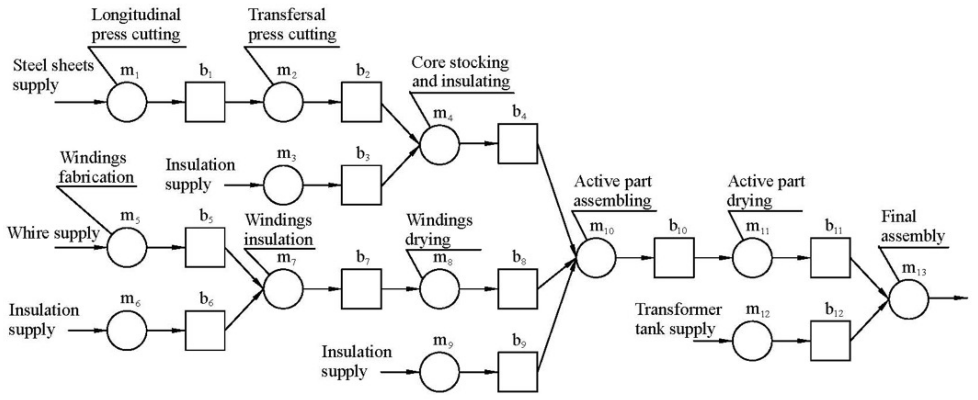
The developed theoretical framework of the finite state method has been applied in the case of power transformer manufacturing, in order to demonstrate its applicability in real-life. The manufacture of power transformers is a complex production process involving numerous operations, yielding a variety of technical solutions, and conditioned on unpredictable customer requirements. Each power transformer is composed of its active and passive parts, and here, we focus on the manufacture of its active part, the essential one. It includes elements in constant contact with voltage and is usually composed of the core, windings, insulating material, and other ancillary components. The core is manufactured out of thin steel sheets cut to a dedicated size using a press-cutter and stacked as a combination of legs (vertical parts) and yokes (horizontal parts) at the core stacking machine. On the other hand, the windings are usually handmade of copper and insulated by several layers of paper or varnish, applying high-quality standards. Upon manufacture, the windings are transferred to a drying device for the improvement of their thermal stability [48]. Once the core and the windings are manufactured, the active part of the power transformer is assembled manually at the assembly work-station and is, upon secondary drying, closed-up within a transformer tank. Usually, the insulating materials as well as the transformer tank are delivered as finished products by external suppliers.

The considered manufacture process is summarized in Figure 14 including a mathematical model of the production process. The reliabilities at the level of each work-station as well as the capacities of the associated buffers acquired using factory-floor measurements are presented in

Table 3. The reliability properties and buffering capacities acquired on the factory floor.

Reliability properties
p1	p2	p3	p4	p5	p6	p7	p8	p9	p10	p11	p12	p13
0.81	0.74	0.90	0.81	0.79	0.90	0.72	0.92	0.90	0.51	0.98	0.90	0.61
Buffer capacities
N1	N2	N3	N4	N5	N6	N7	N8	N9	N10	N11	N12
1000	1000	400	5	1000	400	4	4	200	2	2	2

. The production rate, the work-in-process at each buffer, and the probabilities of blockage and starvation were determined using the finite state method, as outlined in Section 2.2. The obtained results are presented and compared with data provided by the manufacturer in

Table 4. Comparison of the determined key performance indicators with those acquired on the factory floor.

PR

FSM

0.45

Measured

0.47

WIP

WIP1

WIP2

WIP3

WIP4

WIP5

WIP6

WIP7

WIP8

WIP9

WIP10

WIP11

WIP12

FSM

921

868

377

4.7

908

380

3.4

3.9

189

0.5

1.9

1.0

Measured

Full

Full

340

4.5

Full

270

3.8

3.8

194

0.4

1.5

1.2

BL

BL1

BL2

BL3

BL4

BL5

BL6

BL7

BL8

BL9

BL10

BL11

BL12

BL13

FSM

0.30

0.24

0.40

0.30

0.29

0.25

0.43

0.41

0.00

0.53

0.10

0.40

/

Measured *

n/a

n/a

n/a

n/a

n/a

n/a

n/a

n/a

n/a

n/a

n/a

n/a

/

ST

ST1

ST2

ST3

ST4

ST5

ST6

ST7

ST8

ST9

ST10

ST11

ST12

ST13

FSM

/

0.00

/

0.01

/

/

0.01

0.00

/

0.16

0.47

/

0.16

Measured *

/

n/a

/

n/a

/

/

n/a

n/a

/

n/a

n/a

/

n/a

* The probabilities of blockage and starvation could not be measured on the factory floor.

. A quite satisfactory agreement between the results could be noted, especially in terms of the production rate, while some discrepancies regarding the work-in-process were noted due to a rather large amount of fabricated elements. Thus, the discrepancy between the calculated and measured production rate amounted to −4.3% concerning the measured one, while discrepancies between the respective values of the work-in-process at each buffer ranged between −13.2% (WIP₂) and 40.7% (WIP₆). However, in most cases, the discrepancy between the calculated and measured values of the work-in-process remained negligible. Additionally, in some cases, significant probabilities of blockage and starvation could be noted (e.g., BL₁₀, BL₇, BL₈, BL₃, BL₁₂, BL₁, BL₄, BL₅, BL₆, BL₂, ST₁₁, ST₁₀, ST₁₆), which indicates that this assembly system could be significantly improved in terms of bottleneck identification.

5. Conclusions

Production has a significant role in modern society. This role is reflected in aspects of the global market, supply chains, transport systems, global and local development strategies, life quality, and others. Thus, any improvement or decline in production affects many ancillary services. However, each production system may be considered inherently stochastic including both external and internal factors. Therefore, the development and implementation of suitable mathematical models enabling the evaluation of associated key performance indicators as well as the overall equipment efficiency are necessary prerequisites for the development of successful company strategies oriented toward profit increase.

Mathematical modeling of the Bernoulli assembly line was presented in this paper. In the first case, the analytical solution to the problem was developed within the Markovian framework including the formulation of the constitutive transition matrices through the separation of variables. Consecutive multiplication of the constitutive matrices resulted in a transition matrix containing transition probabilities associated with all possible states of the assembly system. This transition matrix was then employed within the eigenvalue problem to determine the probability distribution associated with the steady-state performance of the system and was employed to evaluate the key performance indicators such as the production rate, the work-in-process, and probabilities of blockage and starvation. Although this approach yielded accurate results, it suffered from dimensionality issues (memory storage and CPU requirement) when large-scale and transition-rich systems were considered. Hence, in the second case, the finite state method was developed to tackle issues of the problem of dimensionality and the CPU requirements. The finite state method employs the well-known analytical solution of the two-machine and one buffer problem at the level of finite state elements and reconstructs the system-leveled probability distribution by assuming the independence of events at each buffer. To validate the developed procedure, both methods were applied in several theoretical cases involving three, four, and five machines in different arrangements. A comparison of the obtained results proved the finite state method as a reliable yet CPU-efficient method yielding accurate results, except for some discrepancies attributed to the lowest range of the buffer capacities and induced due to a rather coarse system state discretization. Furthermore, it was concluded that the arrangement of machines in the assembly line does not affect the accuracy of the results. Hence, the FSM can be reliably employed in cases of assembly systems including multiple assembly machines and secondary flows. Following these findings, the application of the finite state method in the case of a realistic assembly line was presented including its validation against the factory floor measurements.

When compared to similar methods available in the literature, FSM stands out as the only method operating in the complete system state space. For this reason, it enables the reconstruction of the steady-state probability distribution while keeping the functional relationship between the properties of an assembly line and the key performance indicators. This fact makes it quite suitable for purposes such as improvability and design considerations. Consequently, it yields predictive analytics suitable for long- and short-term decision-making in the context of production system management and the development of smarter and more efficient production policy.

Finally, it has to be pointed out that the presented approach is still limited to synchronous production systems (serial, splitting, and assembly lines) only involving machines of the Bernoulli reliability. Hence, it faces numerous challenges such as production systems with product quality checking, reworking stations, or customer demands as well as cases of asynchronous production systems, or production systems with machines of geometric and exponential reliability definitions including both steady-state and transient performance. These issues must be addressed in future work to suitably cope with the requirements and concepts of digital twinning, smart factories, and Industry 4.0.