A Multi-Scale Approach for Modelling Airborne Transport of Mucosalivary Fluid

Abstract

COVID-19 pandemic promoted a lot of research activities in relation to mucosalivary fluid airborne transport. Indeed, infection mechanisms are the result of mucosalivary fluid droplets exchange and the knowledge in this area is still largely inadequate. One of the main challenges concerns the modelling of mucosalivary fluid complex nature. Specifically, this is a key element to predict small diameters dry nuclei formation which are highly relevant from the transmission risk point of view. For this reason, in this paper we present and discuss the development of a new multi-scale modelling technique which incorporates the Population Balance Equation into a standard particle-source-in-cell method. Thus, the effectiveness of the aforementioned technique in droplet nuclei generation modelling is showed and discussed. Also the impact of velocity boundary conditions at the mouth print is assessed as well as the effect of the correlations for mass transfer showing that their neglect causes an underestimation in distance reached by the droplets.

1. Introduction

COVID-19, which is a disease caused by the SARS-CoV-2 virus, was recognized as a global pandemic in March 2020 by the World Health Organization (WHO). More than 600 million cases and more than 6 millions deaths were reported worldwide as of September 2022 [1]. SARS-CoV-2 virus airborne transmission was confirmed as the dominant route to spread the virus itself [2]. Moreover, typical infection mechanisms are the discussed in Mittal et al. [3] and they can be classified as follows: $\left(\mathrm{i}\right)$ direct transfer of large saliva droplets to the receiver’s conjunctiva, mouth, or nose; $\left(\mathrm{ii}\right)$ physical contact with droplets deposited on the surface and subsequent absorption to the nasal mucosa of the receiver; and $\left(\mathrm{iii}\right)$ inhalation of respiratory ejected aerosolized particles.

The physical phenomena governing the aforementioned mechanisms are mainly inertia, gravity, buoyancy, aerodynamic drag, and evaporation [4]. In such context, a critical role is related to evaporation which continuously decreases the droplets’ mass until they are reduced to a non-volatile dry nuclei also known as droplet nuclei [5]. Specifically, dry nuclei formation process is strictly related to droplets’ chemical composition as well as the environmental relative humidity and temperature. Hence, it is important to remark that human saliva is more complex than pure water. Indeed, in addition to water, which represents ∼99% of its mass, also mucus, amylase, electrolytes, sodium chloride, white blood cells, epithelial cells, proteins and enzymes are typically contained within saliva droplets [6], creating a complex water solution. In most cases, water’s evaporation can produce a supersaturated solution condition which triggers nuclei crystallization and their growth that is finalized in solid dry particles [7]. Droplet nuclei are also often characterized by small diameters and, for this reason, they are not highly influenced by gravity as larger droplets [8]. Moreover, saliva dry nuclei can reach significant distances remaining airborne for longer periods (up to hours) [9].

Therefore, it is very simple to recognize the complexities of the physical phenomena involved in the propagation of a saliva cloud produced by extra-ordinary respiratory activities. In addition, their deep understanding is essential in order to define appropriate guidelines for face masks wearing as well as social distancing. Unfortunately, distancing rules are insufficient to contain the spread of aerosols carrying SARS-CoV-2. Thus, the physics behind the saliva droplets spread must be also correctly understood also for designing effective engineering solutions to be implemented in closed environments [10].

A lot of review and research papers, relying on numerical and experimental techniques, have been published in the recent months in order to gain new insights into routes of SARS-CoV-2 transmission process and on the efficacy of prevention methods [11,12]. Considering the complex nature of mucosalivary fluid is probably the biggest modeling challenge and only very few papers addressed this topic at the time of this writing [7,13,14,15]. In all the literature cases non-volatile components are replaced by NaCl. However, this approach has been applied to a very limited number of cases to date and, for example, is not still clear the most appropriate concentration of NaCl.

This paper, which is an extended version of our former conference paper [16], presents our latest results in foregoing research area. In particular, a new computational approach, relying on the OpenFOAM library [17], is presented. Special care was devoted to modeling crystallization kinetics triggered from NaCl/water solution supersaturation. Indeed, our approach that will be accurately discussed in the paper, is intended to allow the modelling of droplets’ behaviour at micro–scale level which is activated by meso-scale evaporative phenomena. This research is oriented to advance the state-of-art concerning the saliva chemical composition accounting. Notably, Population Balance Equation (PBE) is solved inside each droplet laden into the domain for the sake of prediction crystallization phenomena.

This paper is organized as follows: the governing equations are reported in Section 2, while the numerical approximations are discussed in Section 3. Numerical results are shown in Section 4. Finally, Section 5 contains the conclusions.

2. Governing Equations

The numerical computations presented in the following are based on an Eulerian–Lagrangian technique described in this section. Specifically, Eulerian and Lagrangian phases are coupled with particle-source-in-cell (PSI-Cell) method [18]. On the other hand, sodium chloride related crystallization kinetics effects are taken into account by solving PBE in combination with PSI-Cell approach.

2.1. Eulerian Phase

Compressible Reynolds Averaged Navier-Stokes (RANS) equations are solved for Eulerian phase:

$$\begin{array}{l}\frac{\partial \overline{\rho }}{\partial t}+\frac{\partial }{\partial x_j}\left(\overline{\rho }{\tilde{u}}_j\right)=,\\ \frac{\partial }{\partial t}\left(\overline{\rho }{\tilde{u}}_i\right)+\frac{\partial }{\partial x_j}\left(\overline{\rho }{\tilde{u}}_i{\tilde{u}}_j\right)=-\frac{\partial \overline{p}}{\partial x_i}+\frac{\partial {\widehat{\tau }}_{ij}}{\partial x_j}+\overline{\rho }g{\delta }_{i3}+s_{m,i},\\ \frac{\partial }{\partial t}\left(\overline{\rho }\tilde{E}\right)+\frac{\partial }{\partial x_j}\left(\overline{\rho }{\tilde{u}}_j\tilde{H}\right)=-\frac{\partial q_j}{\partial x_j}+\frac{\partial }{\partial x_j}\left({\tilde{u}}_i{\widehat{\tau }}_{ij}\right)+s_e,\\ \frac{\partial }{\partial t}\left(\overline{\rho }{\tilde{Y}}_k\right)+\frac{\partial }{\partial x_j}\left(\overline{\rho }{\tilde{u}}_j{\tilde{Y}}_k\right)=-\frac{\partial m_{k,j}}{\partial x_j}+s_{Y_k},\end{array}$$

(1)

where $\overline{\rho }$, ${\tilde{u}}_i$, $\overline{p}$ and ${\tilde{Y}}_k$ denote density, velocity component in $x_i$ direction, pressure, temperature and chemical specie k mass fraction. $\tilde{E}$ and $\tilde{H}$ are, respectively, the total internal energy and enthalpy. As usual in CFD community, the overbar and the tilde are filtering operators which are introduced for unweighted and density-weighted averages.

In Equation (1) we can find several unclosed terms which handled in a standard way, i.e., rheological equation for newtonian fluids, Fourier law and Fick law are employed. Conversely, Reynolds stresses are modelled using SST k–$\omega$ model developed by Menter [19]. It is also important to note that the source terms in Equation (1) are the mathematical expression of the Lagrangian and Eulerian phases coupling [18].

2.2. Lagrangian Phase

The velocity and the position of the particles laden into the computational domain are the results of the momentum and trajectory equations. In this paper we adopt a two-way coupling between carrier fluid and Lagrangian phase. Thus, non-collisional spherical particles are scrutinized. Saliva droplets, considered in this paper, exhibit a diameters’ range such that pressure, virtual mass and Brownian forces can be neglected [20,21]. Furthermore, the Weber number calculated for the droplets’ velocities considered in this work, is such that no secondary break-up phenomena occur. For the above reasons is possible to study each discrete particle including: gravity, aerodynamic drag and buoyancy. Aerodynamic drag coefficient is obtained from standard Putnam correlation for spheres [22]. By contrast, the convective heat transfer coefficient and the mass transfer one are obtained from two different approaches summarized in

Table 1. Correlations for Nusselt and Sherwood numbers.

	Nu	Sh
Ranz–Marshall [23]	$2+0.6{\mathrm{Re}}_d^{0.6}{\mathrm{Pr}}^{\frac{1}{3}}$	$2+0.6{\mathrm{Re}}_d^{0.6}{\mathrm{Sc}}^{\frac{1}{3}}$
Clift [24]	${\left(1+\mathrm{Re}·\mathrm{Pr}\right)}^{\frac{1}{3}}·max\left[1,{\mathrm{Re}}_d^{0.77}\right]$	${\left(1+\mathrm{Re}·\mathrm{Sh}\right)}^{\frac{1}{3}}·max\left[1,{\mathrm{Re}}_d^{0.77}\right]$

. Specifically, ${\mathrm{Re}}_d$ is the Reynolds number evaluated on the particles’ diameter, while $\mathrm{Pr}$ and $\mathrm{Sc}$ represent Prandtl and Schmidt numbers, respectively.

The droplets’ initial diameter is assessed through a Rosin–Rammler distribution [25]:

$$f=\frac{n}{{\overline{D}}_P}{\left(\frac{D_{P,i}}{{\overline{D}}_P}\right)}^{n-1}exp\left[-{\left(\frac{D_{P,i}}{{\overline{D}}_P}\right)}^n\right];$$

(2)

the parameters required by Equation (2) are calibrated on the basis of Xie et al. [26] experimental data [27]. Specifically, n was fixed equal to 8 while average parcels’ diameter, ${\overline{D}}_p$ was set equal to o 80 µm. In Equation (2) $D_{P,i}$ represents the i-th particle’s diameter. Lastly, the minimum diameter of the injected parcels is 10 µm, while the maximum one is 280 µm.

2.3. PSI–PBE Coupling

One of the main novelty of this work is related to the coupling between PSI-Cell method and PBE. Precisely, PBE is solved in the droplet’s inner part in order to model nucleation and growth processes of the $\mathrm{NaCl}$ crystals.

PBE solution enables the possibility to predict droplet nuclei generation phenomenon. In this context, PBE is reformulated ignoring spatial terms, i.e., both convective and diffusive terms are removed. This is possible due to the homogeneous spatial condition of the considered system. Hence, PBE collapses in an ordinary differential equation which requires limited computational resources for its solution. Moreover, a similar formulation is also attractive from the numerical point of view because of its increased numerical stability. PBE reads as follows [28]:

$$\frac{\partial N_j}{\partial t}+\nabla ·\left(N_j{\mathbf{u}}_p\right)-\nabla ·\left(D_t{N}_j\right)=-\sum _j\frac{\partial \left[G_j{N}_j\right]}{\partial r_j}+B\prod _j\delta \left(r_j-r_{j0}\right)+h$$

(3)

where $N_j$ is density number of i-th chemical specie, $D_t$ is the local turbulent diffusivity, $G_j$ is the growth rate, $r_j$ is the particle internal coordinate, $r_{j0}$ is the particle internal coordinate for a crystal nucleus. Furthermore, $\delta$ is the Dirac function, B is the nucleation rate, and h is the creation or destruction of particles due to aggregation, agglomeration, and breakage.

The interest of this paper is limited to crystallization phenomena issues of NaCl. Consequently, PBE needs to include only B and G terms. Moreover, the convective and diffusive terms for the particles disappear because we assume each droplet to be well mixed and tracked independently in the Lagrangian frame.

It is feasible to re-write PBE in a semi-discrete form integrating Equation (3) over r:

$$\frac{d{f}_j}{dt}=-\frac{1}{\Delta r}\left[G_{j+1/2}\left(f_j+\frac{\Delta r}{2}{\left(f_r\right)}_j\right)-G_{j-1/2}\left(f_{j-1}+\frac{\Delta r}{2}{\left(f_r\right)}_{j-1}\right)\right]$$

(4)

where $f_j$ is the particle-averaged population density. It is also important to remark that in Equation (4) nucleation term is included averaging the nucleation rate within discrete linear computational cells built inside the droplets. Starting from Woo et al. [28], it is possible to evaluate particle-averaged crystal mass:

$$N_{w,j}=\frac{1}{4}{\rho }_c{k}_v{f}_j\left(r_{j+1/2}^4-r_{j-1/2}^4\right)$$

(5)

which, in turns, allows to calculate the total mass related to crystallization process as:

$$m_{cr,i}=\pi \frac{D_{p,i}^3}{6}\sum _j{N}_{w,j}$$

(6)

and the radius of the (dry) solid part of the droplets, $r_N$:

$$r_N=\frac{{\sum }_j{N}_{w,j}{r}_j^4}{{\sum }_j{N}_{w,j}{r}_j^3};$$

(7)

actually, combining Equations (5) and (6), semi-discrete PBE can be formulated as:

$$\begin{array}{cc}\hfill \frac{d{N}_{w,j}}{dt}=& -\frac{\rho k_v}{4\Delta r}\left(r_{j+1/2}^4-r_{j-1/2}^4\right)max\left(\mathrm{sign}\Delta c,0\right)\times \hfill \\ \hfill & \left[G_{j+1/2}\left(f_j+\frac{\Delta r}{2}{\left(f_r\right)}_j\right)-G_{j-1/2}\left(f_{j-1}+\frac{\Delta r}{2}{\left(f_r\right)}_{j-1}\right)+\underset{j=0}{\underbrace{B}}\right].\hfill \end{array}$$

(8)

In the above equation $\Delta c$ = $c-c^{*}$ is supersaturation, while c and $c^{*}$ are the NaCl concentration and its solubility in pure water. Since particles’ temperature variation in almost negligible, then $c^{*}$ dependence from the temperature is not here considered; thus, we have fixed $c^{*}=0.36$ g NaCl/g H₂O. Finally, nucleation and growth rates coefficients are evaluated using literature correlations for NaCl/water solutions [29,30]:

$$\begin{array}{cc}\hfill & G=2\sqrt{\frac{1.3·{10}^{-9}}{\pi t_{cr}}}\left(c-c^{*}\right),\hfill \\ \hfill & B=A_{b}exp\left(-r_s\right).\hfill \end{array}$$

(9)

In Equation (9) $t_{cr}$ represents the time passed from crystallization process beginning; on the other hand $A_b$ is a constant value and it is equal to $9.78304·{10}^{28}$, while $r_s$ is evaluated as follows:

$$r_s=\frac{\pi {\left(\frac{c}{c^{*}}\right)}^{0.1642}}{{\left(log\frac{c}{c^{*}}\right)}^{2.52\frac{c}{c^{*}}}}.$$

(10)

It is also important to remark that particle density, ${\rho }_P$, is updated during crystals’ growth as follows:

$${\rho }_P=\left(1-x_m\right){\rho }_{{\mathrm{H}}_2\mathrm{O}}+x_m{\rho }_{\mathrm{NaCl}}$$

(11)

where $x_m$ is the sodium chloride mass fraction in its dilute solution with water. As can be easily understood this value changes in each time step due to water evaporation and it is used to re-compute the particles’ diameter.

3. Numerical Approximation

The Eulerian phase governing equations were space discretized using an unstructured collocated cell-centered finite volume approach. Time-integration relied on an implicit second-order scheme with an adjustable time stepping strategy. Additionally, the local Courant $\mathrm{Co}$ was fixed to be lesser a user-defined value, i.e., ${\mathrm{Co}}_{\max }$. In the computations presented in the following ${\mathrm{Co}}_{\max }$ was fixed equal to $0.2$.

A linear-upwind scheme was used for convective fluxes interpolation handling. Differently, a central scheme was adopted for diffusive terms. Pressure–Implicit with Splitting Operators (PISO) procedure [31], was assumed as pressure–velocity decoupling strategy. Distinct solution strategies were considered for the linear solvers deriving space-time discretization. A preconditioned conjugate gradient (PCG) method was used to solve the Poisson equation for pressure; a diagonal incomplete–Cholesky preconditioner was borrowed. All other systems deriving from the remaining equations were solved using a preconditioned bi-conjugate gradient (PBiCG) method. The Diagonal Incomplete Lower Upper (DILU) preconditioner was applied in these cases. Furthermore, a local accuracy of ${10}^{-7}$ was established for the pressure, whereas other linear systems were considered as converged when the residuals reached the machine precision.

Lagrangian phase momentum and mass equations were solved using a backward Euler scheme for time-integration. By contrast, energy equation for particles was solved analytically. A critical point of our solution strategy is related to PBE. Indeed, several numerical instabilities issues were encountered in our computational experience. To avoid the blow-up of the computations we use an explicit Strong Stability Preserving Runge-Kutta (SSPRK) having 9 stages and 5-th order of accuracy [32]. The adoption of this scheme is particularly appealing since it allows to use same time-step size for all the involved scales. Moreover, ${\left(f_r\right)}_j$ terms, are approximated by the min-mod limiter [28].

Initial and Boundary Conditions

In the present work, a 3D computational domain, represented in Figure 1, was employed; it consists of an open air volume starting from the mouth print of a standing coughing person. A length $L=4$ $\mathrm{m}$, a width $W=1$ $\mathrm{m}$, and a height $H=3$ $\mathrm{m}$ were adopted for the entire domain, in accordance with Dbouk and Drikakis [27]. The reference frame origin, $O=\left(0,0,0\right)$, is placed in the same plane where the mouth print itself is inserted. It is worth noting that x-axis is aligned with the streamwise direction, i.e., $0\le x\le 4$; y-axis is the transverse direction: $-0.5\le y\le 0.5$. Lastly, z-axis is employed for vertical direction, thus $0\le z\le 3$. Moreover, the mouth print shape was approximated to be rectangular with an area of $2\times {10}^{-4}$ ${\mathrm{m}}^2$ and its center, $P_m$, was placed in the same position selected by Dbouk and Drikakis: $P_m=\left(0,0,1.63\right)$ [27]. The reason behind this choice is due to the fact a regular shape allows to use a fully orthogonal hexahedral cells. Furthermore, the number of grid cells is fixed to $5.83\times {10}^6$ which is the result of our former investigations about the solution space-time convergence [33].

For the sake of discussing the employed boundary conditions (BCs), it is noteworthy to mention that, for all the simulations presented below, both the Eulerian and Lagrangian phases are introduced from the mouth print boundary at $x=0$ $\mathrm{m}$. The remaining part of the y–z plane at $x=0$ $\mathrm{m}$ is such that all the variables have a null gradient through it. The ground is handled as a standard viscous wall. Differently, symmetry conditions are used on lateral boundaries. Zero gradient condition is also set for all the variables at the domain top with the exception of the pressure. Specifically, the pressure is reduced to its hydrostatic level. The y–z plane at $x=4$ $\mathrm{m}$ is handled as a physical outflow. By contrast, the pressure is imposed to decrease linearly, starting from the atmospheric pressure level at $z=0$ $\mathrm{m}$.

The initial temperature of the carrier fluid is 20 °C with relative humidity fixed at 50%. The ground is at 25 °C, while the air and droplets ejected by human mouth are at 34 °C. No background flow is included in the presented computations. However, initial fields consistent with atmospheric conditions were adopted. These fields are obtained through a preliminary computation which does not provide Lagrangian particles into the domain. It should be noted that cloud evolution is strongly influenced by this conditions [33].

In order to mimic the mass injection from human mouth two different strategies were adopted, see Figure 2. A first approach consists in imposing a stepped velocity inlet at the mouth boundary. A stream-wise velocity inlet step, having an amplitude equal to 8.5 m/s, was applied over 0.12 s. These values were deduced on the basis of measurements carried out by Scharfman et al. [34].

Secondly, following Cortellessa et al. [35], a sinusoidal approximation of breathing, hereinafter coughing/breathing configuration, is adopted to simulate a real-life condition. In particular, the transient sinusoidal velocity profile presents an amplitude of 1 m/s and a frequency of 0.2 Hz. A velocity peak of 5 m/s was also mounted on the sinusoidal velocity profile in order to reproduce coughing effect as showed by Abkarian et al. [36]. In both the configurations, carrier fluid and injected particles were subjected to the same velocity condition. Note also that, for the second strategy, particles are injected only during the velocity peak. Moreover, turbulence intensity, Tu, is fixed at 15% and the mixing length is equal to $7\times {10}^{-3}$ at the mouth boundary.

As regards saliva droplets, it is important to put in evidence that total mass laden into the domain for a single cough event is 7.7 mg, according to the experimental measurements performed by Xie et al. [26] and CFD simulations [27,33]. When breathing is simulated, no further Lagrangian particles are introduced. Lastly, as already explained in Section 1, saliva is handled as NaCl completely diluted in water. The related concentration value are obtained from Rosti et al. [7]. Specifically, NaCl mass is fixed equal to 1% of initial droplet’s mass.

4. Results

In this section we present the numerical results referred to the saliva droplets’ cloud produced during coughing. Some cloud characteristics are computed in order to investigate its diffusion: the center of mass and fraction of particles present in a reference volume. The cloud center of mass is defined as:

$$\mathbf{G}=\frac{{\sum }_{i=1}^{N_p\left({\Omega }_0\right)}{m}_{P,i}{\mathbf{x}}_{P,i}}{{\sum }_{i=1}^{N_p\left({\Omega }_0\right)}{m}_{P,i}},$$

(12)

where $N_p\left({\Omega }_0\right)$ is the number of parcels laden in the overall domain, ${\Omega }_0$, in a given time-instant. In the following, $\mathbf{G}=\left(x_G,y_G,z_G\right)$ is considered as the center of mass components. By contrast, the ratio between the number of particles present in a reference volume, ${\Omega }_i$, and the total number of particles in ${\Omega }_0$ (in a given time instant) is used to track the droplets’ population distribution in a possible risk zone. The reference index [33], is defined as:

$${\Phi }_{{\Omega }_i}=\frac{{\sum }_{k=1}^{N_p\left({\Omega }_i\right)}{N}_{p,k}}{{\sum }_{k=1}^{N_p\left({\Omega }_0\right)}{N}_{p,k}},$$

(13)

the aforementioned reference volume, ${\Omega }_i$, is parallelepipedal type having the following features:

$${\Omega }_i=[0,{\alpha }_i]\times \left[-0.5,0.5\right]\times \left[1.3,1.8\right].$$

(14)

The parameter ${\alpha }_i$, appearing in Equation (14), spans the following values: $1.0$ $\mathrm{m}$, $1.2$ $\mathrm{m}$ and $1.5$ $\mathrm{m}$. ${\Omega }_i$ stream-wise dimensions were selected in order to investigate the effectiveness of 1 $\mathrm{m}$ distance, which is the safety distance adopted in Italy during pandemic. The transverse direction range is considered in order to completely cover the domain. Lastly, the z-axis interval is defined as useful to assess possible direct contamination mechanism in a one-to-one close contact situation. The impact of droplets’ evaporation is estimated using the particles weighted average diameter, $D_{10}$:

$$D_{10}=\frac{{\sum }_{i=1}^{N_p\left({\Omega }_0\right)}{N}_{P,i}{D}_{P,i}}{{\sum }_{i=1}^{N_p\left({\Omega }_0\right)}{N}_{P,i}}.$$

(15)

All the computations here presented were performed on the HPC-system CRESCO6 hosted by ENEA at Portici (Italy). CRESCO6 is made up 434 nodes with two Intel Xeon Platinum 8160 of the Skylake (SKL) generation operating at 2.1 GHz for each node. The processors have 24-cores each one. There are 192 GB of RAM available in standard nodes. Finally, the codes were built using Intel compilers and the MPI library version developed by Intel. It should be noted that the typical computation time of a single case is about 24 h run in parallel using 384 CPU-cores on CRESCO6.

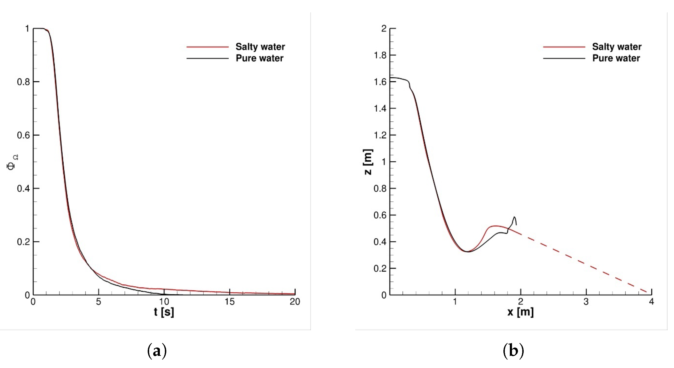
4.1. Impact of Saliva Chemical Composition

In this section we discuss the impact of NaCl presence within droplets comparing their kinematic behaviour with pure water particles. Note that for this analysis we use the same injection strategy for particles’ diameters selection, see Section 2.2. In addition, only Ranz–Marshall correlations for particles’ $\mathrm{Nu}$ and $\mathrm{Sh}$ and stepped velocity time-history at the inlet boundary are considered.

Looking at Figure 3a,b, it is very straightforward to note the effect of the different mucosalivary fluid chemical compositions here considered. Indeed, after 4 $\mathrm{s}$ from the emission, the reference control volume which is evidenced with the red lines, $\left({\alpha }_i=1\mathrm{m}\right)$, is occupied by almost the same number of particles for both the cases. Nevertheless, it is also easy to observe that clouds shape is fairly different. This evidence can be explained with reference to droplets’ density. Indeed, initial diameters distribution is the same for the two cases. Thus, the deriving particles’ kinematic behaviour is affected in a non-negligible way on the basis of their chemical composition. Moreover, up to $t=4$ $\mathrm{s}$ the crystallization kinetics is still in a premature stage to have notably effect on particles evolution, see Figure 3b.

Otherwise, in Figure 4a,b, at $t=10$ $\mathrm{s}$ the effect of NaCl crystallization process produces an evident impact on the discrete phase space distribution. This is mainly related to the effects that can be observed only when salty droplets interaction with the surrounding environment is taken into account. In fact, the PBE adoption at particle level allows to capture dry nuclei formation at a possible receiver’s height and having small diameters. This phenomenon is totally neglected in case of pure water droplets because their complete evaporation occurs after few seconds from their emission. On the other hand, the crystallization process modeling, produces a time-dependent density variation within the droplets that shows a significant impact on the cloud dynamics.

In particular, the risk area is sensibly more populated, even for a stream-wise length greater than 1 $\mathrm{m}$, when salty droplets are considered. This evidence is also expressed quantitatively from ${\varphi }_{\Omega }$ time-history represented in Figure 5a.

The center of mass trajectory on the x–z plane, depicted in Figure 5b, shows a peculiar behaviour. It is very clear that in an initial stage, $0.35\mathrm{m}<x_G<1\mathrm{m}$, the $z_G=f\left(x_G\right)$ curve is almost linear due to the cancellation of inertial terms. By contrast, for grater distances the crystallization effects have a relevant effect and the $z_G$ curve is not linear anymore. It is worth noting that, for stream-wise distances greater than 2 $\mathrm{m}$ from the mouth print, the $z_G=f\left(x_G\right)$ curve is extrapolated. This is possible since Lagrangian particles move into the domain with an uniform velocity. It is really evident that dry nuclei are able to reach distances sensibly longer than pure water droplets which completely evaporates from the domain in less than 20 $\mathrm{s}$. Additionally, dry particles have average diameter approximately around 10 $\mathsf{\mu }\mathrm{m}$. For this reason a fly time having an order of magnitude of 60 $\mathrm{s}$ is expected.

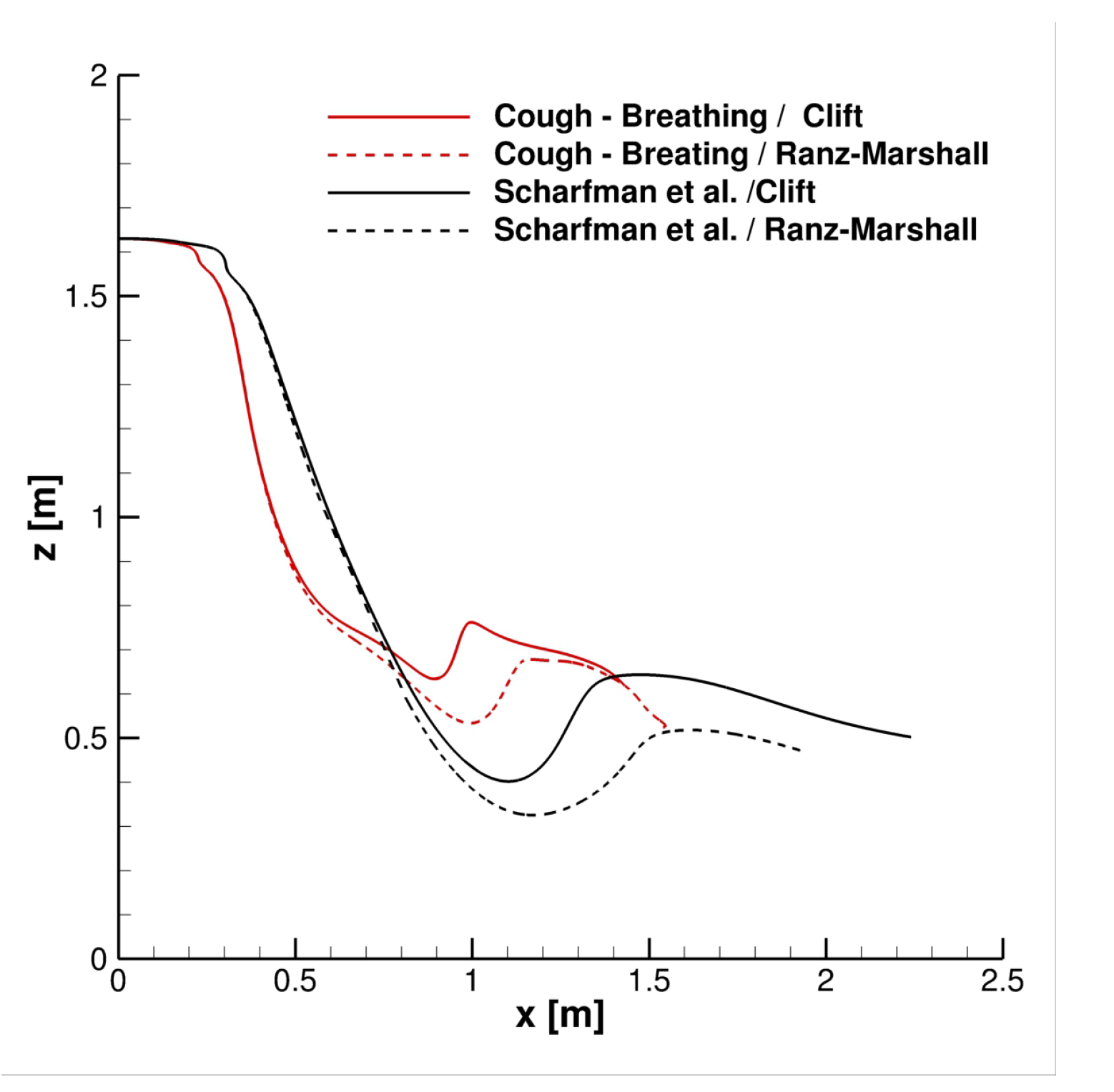
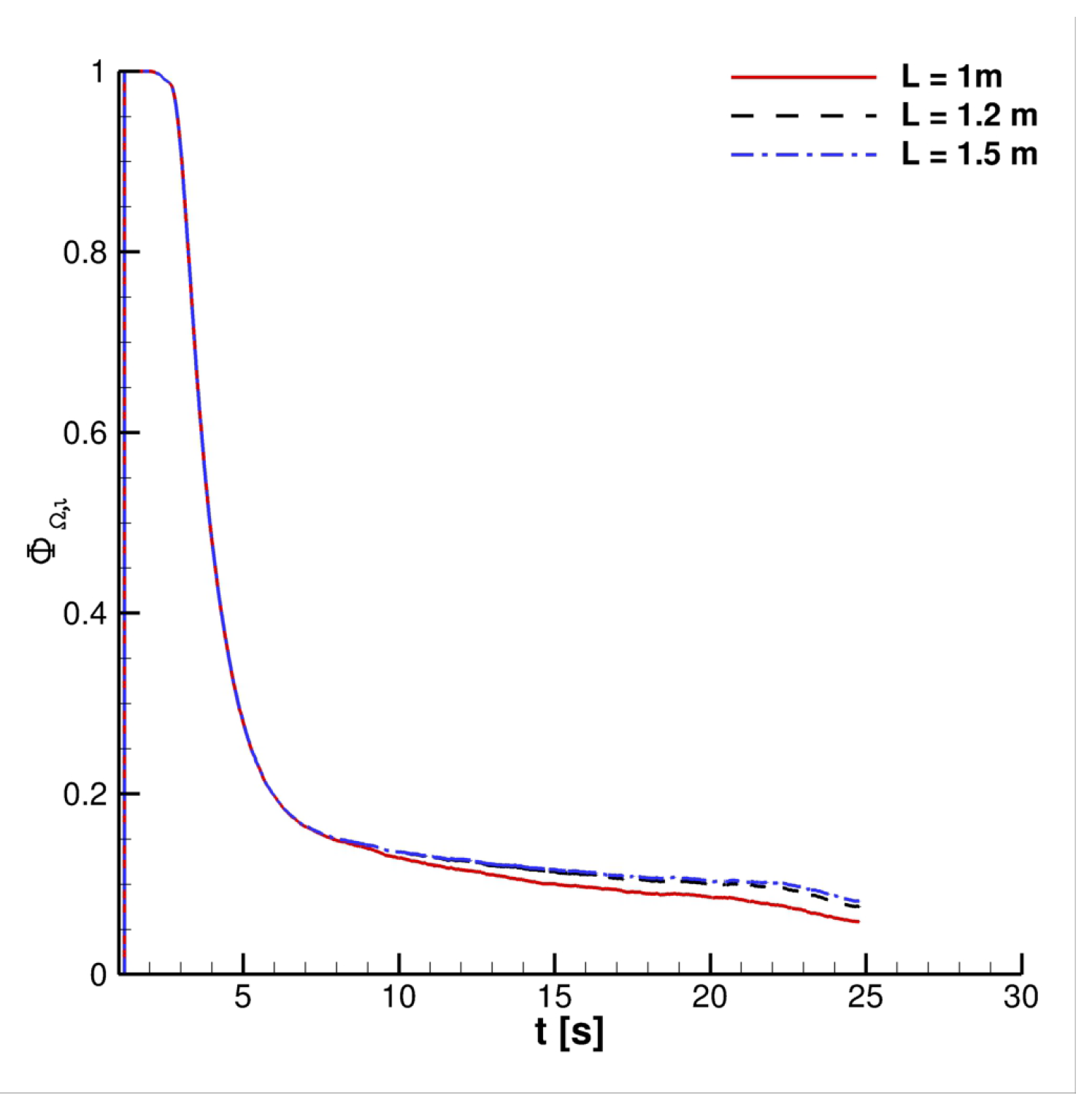
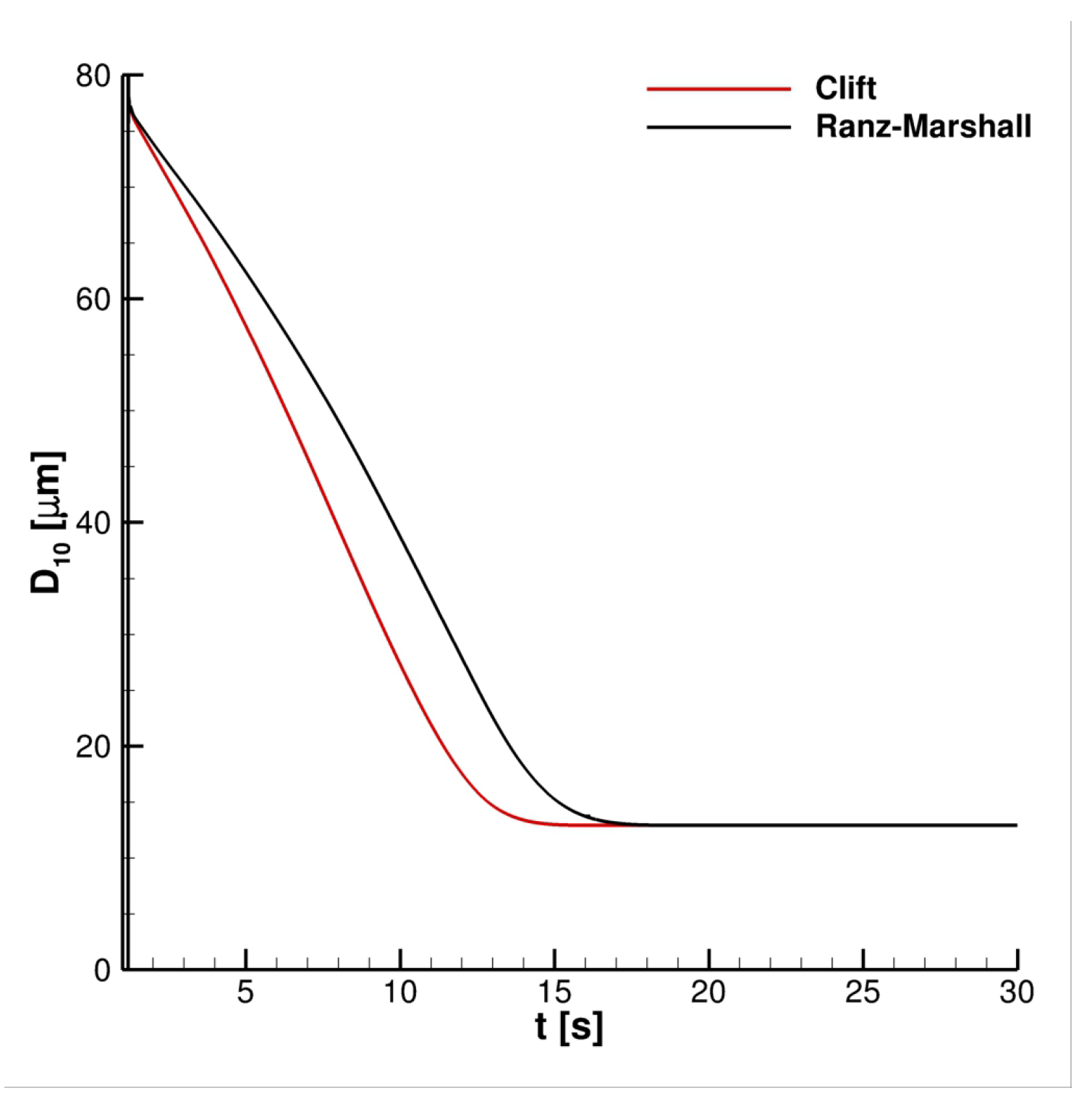
4.2. Effect of Velocity Inlet Time-Histories

In this subsection we discuss the impact of the different velocity time-history profiles at inlet boundary as well as the overall effect of the two approaches here considered for particles’ $\mathrm{Nu}$ and $\mathrm{Sh}$ numbers evaluation (see Section 2.2). For this specific case, only salty droplets are used because of they are closer to physical reality.

Looking at Figure 6 it is very easy to note that the saliva cloud’s center of mass is influenced from both BCs and $\mathrm{Nu}$/$\mathrm{Sh}$ approaches. Specifically, for both the velocity inlet BCs strategies, Clift correlations for $\mathrm{Nu}$/$\mathrm{Sh}$ numbers produce an higher average center of mass height from the ground. This is a clear consequence of a reduced evaporation rate of Clift correlations if compared with Ranz–Marshall ones. It should be pointed out that stepped velocity at inlet produces an average $z_G$ lesser than coughing/breathing configuration. This evidence is clearly related to the average values of the particles’ momentum laden into the domain. Indeed, with the stepped approach, particles are injected with a velocity equal to $8.5$ $\mathrm{m}/\mathrm{s}$, while in coughing/breathing configuration particles’ velocity during cough is 5 $\mathrm{m}/\mathrm{s}$. Thus, it is very easy to understand the reason why particles are able to fall down easier in the stepped velocity configuration at the mouth print.

Therefore, Figure 6 clearly emphasizes that from transmission risk point of view coughing/breathing configuration coupled Clift configuration is the more relevant. For this reason, Figure 7 shows ${\Phi }_{{\Omega }_i}\left(t\right)$ curve for the aforementioned setup. It is quite easy to note that, for stream-wise distances ranging from 1 $\mathrm{m}$ to $1.5$ $\mathrm{m}$, ${\Phi }_{{\Omega }_i}$ curves are very similar each other. More in depth, particles’ number concentration estimated with coughing/breathing configuration and Clift correlations, after 20 $\mathrm{s}$ from the emission, is approximately twice if compared with stepped velocity inlet and Ranz–Marshall correlations data showed in Figure 5a.

In Figure 8 $D_{10}\left(t\right)$ plot is showed. It is to be noted that $D_{10}$ approaches average particles’ diameters. For both the cases represented in Figure 8, it is very clear to note that a locked final diameter value is reached. This is due to the formation of dry particles nuclei. Clift correlation and Ranz–Marshall ones differ only for the time required to reach terminal diameter because they impose different evaporation rates. The data showed in Figure 8 are very encouraging, since the ratio between terminal diameter and the initial one, $D/D_0$, is $0.161$ which is in fairly good agreement with literature data. Indeed, Lieber et al. [37] showed experimentally, on real mucosalivary fluid, that $0.18\le D/D_0\le 0.2$. It is worth noting that in our modeling strategy, human saliva is handled as a dilute NaCl solution in water. Thus, our data can be considered sufficiently reliable in comparison with real mucosalivary fluid.

5. Conclusions

This paper presents a new multi-scale approach for the prediction of the generation solid dry nuclei deriving from human saliva. The main point of novelty is the introduction the solution of PBE at droplet level into an Eulerian–Lagrangian technique. In particular, a coupling method between PSI-Cell method and PBE was proposed and discussed. In this context, it was showed that NaCl presence has a relevant effect on the saliva droplets kinematic behaviour. Additionally, the evaporation process leads to an increase in droplets’ density due to the growing NaCl concentration. The aforementioned processes have a significant impact on cloud dynamics. More in depth, the adoption of pure water droplets produces an underestimation of the distance reached by the droplets theirselves. Furthermore, we have also noted that velocity time-histories applied at inlet boundary, as well as $\mathrm{Nu}$/$\mathrm{Sh}$ correlations, strongly affect saliva cloud evolution.

The presented approach can be considered sufficiently reliable since numerical data put in evidence a satisfactory agreement with experimental literature data produced on real human saliva in terms of final diameters prediction. Finally, it is should be pointed out that distances ranging from $1.0$ $\mathrm{m}$ to $1.5$ $\mathrm{m}$ are almost equivalent in terms of transmission risk. Thus, it is crucial, for possible future events, to better understand the processes discussed in this paper.

References

1. WHO Coronavirus (COVID-19) Dashboard. Available online: https://covid19.who.int (accessed on 1 October 2022).
2. Zhang, R.; Li, Y.; Zhang, A.L.; Wang, Y.; Molina, M.J. Identifying airborne transmission as the dominant route for the spread of COVID-19. Proc. Natl. Acad. Sci. USA 2020, 117, 14857–14863. [Google Scholar] [CrossRef] [PubMed]
3. Mittal, R.; Ni, R.; Seo, J.H. The flow physics of COVID-19. J. Fluid Mech. 2020, 894, F2. [Google Scholar] [CrossRef]
4. Xie, X.; Li, Y.; Chwang, A.T.Y.; Ho, P.L.; Seto, W.H. How far droplets can move in indoor environments—Revisiting the Wells evaporation-falling curve. Indoor Air 2007, 17, 211–225. [Google Scholar] [CrossRef]
5. Liu, L.; Wei, J.; Li, Y.; Ooi, A. Evaporation and dispersion of respiratory droplets from coughing. Indoor Air 2017, 27, 179–190. [Google Scholar] [CrossRef] [PubMed]
6. van Doremalen, N.; Bushmaker, T.; Morris, D.H.; Holbrook, M.G.; Gamble, A.; Williamson, B.N.; Tamin, A.; Harcourt, J.L.; Thornburg, N.J.; Gerber, S.I.; et al. Aerosol and Surface Stability of SARS-CoV-2 as Compared with SARS-CoV-1. N. Engl. J. Med. 2020, 382, 1564–1567. [Google Scholar] [CrossRef] [PubMed]
7. Rosti, M.E.; Olivieri, S.; Cavaiola, M.; Seminara, A.; Mazzino, A. Fluid dynamics of COVID-19 airborne infection suggests urgent data for a scientific design of social distancing. Sci. Rep. 2020, 10, 22426. [Google Scholar] [CrossRef] [PubMed]
8. Bourouiba, L.; Dehandschoewercker, E.; Bush, J.W.M. Violent expiratory events: On coughing and sneezing. J. Fluid Mech. 2014, 745, 537–563. [Google Scholar] [CrossRef]
9. Bourouiba, L. Turbulent Gas Clouds and Respiratory Pathogen Emissions: Potential Implications for Reducing Transmission of COVID-19. JAMA J. Am. Med. Assoc. 2020, 323, 1837–1838. [Google Scholar] [CrossRef]
10. Faleiros, D.; van den Bos, W.; Botto, L.; Scarano, F. TU Delft COVID-app: A tool to democratize CFD simulations for SARS-CoV-2 infection risk analysis. Sci. Total. Environ. 2022, 826, 154143. [Google Scholar] [CrossRef] [PubMed]
11. Pourfattah, F.; Wang, L.P.; Deng, W.; Ma, Y.F.; Hu, L.; Yang, B. Challenges in simulating and modeling the airborne virus transmission: A state-of-the-art review. Phys. Fluids 2021, 33, 101302. [Google Scholar] [CrossRef] [PubMed]
12. Mohamadi, F.; Fazeli, A. A Review on Applications of CFD Modeling in COVID-19 Pandemic. Arch. Comput. Methods Eng. 2022, 29, 3567–3586. [Google Scholar] [CrossRef] [PubMed]
13. Li, H.; Leong, F.Y.; Xu, G.; Ge, Z.; Kang, C.W.; Lim, K.H. Dispersion of evaporating cough droplets in tropical outdoor environment. Phys. Fluids 2020, 32, 113301. [Google Scholar] [CrossRef] [PubMed]
14. Stiti, M.; Castanet, G.; Corber, A.; Alden, M.; Berrocal, E. Transition from saliva droplets to solid aerosols in the context of COVID-19 spreading. Environ. Res. 2022, 204, 112072. [Google Scholar] [CrossRef] [PubMed]
15. Luo, Q.; Ou, C.; Hang, J.; Luo, Z.; Yang, H.; Yang, X.; Zhang, X.; Li, Y.; Fan, X. Role of pathogen-laden expiratory droplet dispersion and natural ventilation explaining a COVID-19 outbreak in a coach bus. Build. Environ. 2022, 220, 109160. [Google Scholar] [CrossRef] [PubMed]
16. D’Alessandro, V.; Falone, M.; Giammichele, L.; Ricci, R. A multiscale approach for modelling saliva droplets airborne transport in relation to SARS-CoV-2 transmission. In Proceedings of the 6th AIGE/IIETA International Conference and XV AIGE Conference, Ancona, Italy, 8–9 July 2021. [Google Scholar]
17. Weller, H.; Tabor, G.; Jasak, H.; Fureby, C. A tensorial approach to computational continuum mechanics using object-oriented techniques. Comput. Phys. 1998, 12, 620–631. [Google Scholar] [CrossRef]
18. Crowe, C.T.; Sharma, M.P.; Stock, D.E. The Particle-Source-In Cell (PSI-CELL) Model for Gas-Droplet Flows. J. Fluid Eng. 1977, 99, 325–332. [Google Scholar] [CrossRef]
19. Menter, F. Two-Equation Eddy Viscosity Turbulence Models for Engineering Applications. AIAA J. 1994, 32, 1598–1695. [Google Scholar] [CrossRef] [Green Version]
20. Busco, G.; Yang, S.; Seo, J.; Hassan, Y.A. Sneezing and asymptomatic virus transmission. Phys. Fluids 2020, 32, 073309. [Google Scholar] [CrossRef] [PubMed]
21. Abuhegazy, M.; Talaat, K.; Anderoglu, O.; Poroseva, S.V. Numerical investigation of aerosol transport in a classroom with relevance to COVID-19. Phys. Fluids 2020, 32, 103311. [Google Scholar] [CrossRef]
22. Putnam, A. Integratable form of droplet drag coefficient. ARS J. 1961, 31, 1467–1468. [Google Scholar]
23. Ranz, W.E.; Marshall, W.R. Evaporation from drops. Chem. Eng. Prog. 1952, 48, 141–146. [Google Scholar]
24. Clift, R.; Grace, J.R.; Weber, M.E. Bubbles, Drops, and Particles; Dover Publications, Inc.: New York, NY, USA, 2005. [Google Scholar]
25. Mugele, R.A.; Evans, H.D. Droplet Size Distribution in Sprays. Ind. Eng. Chem. 1951, 43, 1317–1324. [Google Scholar] [CrossRef]
26. Xie, X.; Li, Y.; Sun, H.; Liu, L. Exhaled droplets due to talking and coughing. J. R. Soc. Interface 2012, 6, S703–S714. [Google Scholar] [CrossRef] [PubMed] [Green Version]
27. Dbouk, T.; Drikakis, D. On coughing and airborne droplet transmission to humans. Phys. Fluids 2020, 32, 053310. [Google Scholar] [CrossRef] [PubMed]
28. Woo, X.Y.; Tan, R.B.H.; Chow, P.S.; Braatz, R.D. Simulation of Mixing Effects in Antisolvent Crystallization Using a Coupled CFD-PDF-PBE Approach. Cryst. Growth Des. 2006, 6, 1291–1303. [Google Scholar] [CrossRef]
29. Desarnaud, J.; Derluyn, H.; Carmeliet, J.; Bonn, D.; Shahidzadeh, N. Metastability Limit for the Nucleation of NaCl Crystals in Confinement. J. Phys. Chem. Lett. 2014, 5, 890–895. [Google Scholar] [CrossRef] [Green Version]
30. Naillon, A.; Joseph, P.; Prat, M. Sodium chloride precipitation reaction coefficient from crystallization experiment in a microfluidic device. J. Crys. Growth 2017, 463, 201–210. [Google Scholar] [CrossRef] [Green Version]
31. Issa, R.I. Solution of the implicitly discretised fluid flow equations by operator-splitting. J. Comput. Phys. 1986, 62, 40–65. [Google Scholar] [CrossRef]
32. Ruuth, S.J.; Spiteri, R.J. High-Order Strong-Stability-Preserving Runge-Kutta Methods with Downwind-Biased Spatial Discretizations. SIAM J. Numer. Anal. 2005, 42, 974–996. [Google Scholar] [CrossRef]
33. D’Alessandro, V.; Falone, M.; Giammichele, L.; Ricci, R. Eulerian–Lagrangian modeling of cough droplets irradiated by ultraviolet–C light in relation to SARS-CoV-2 transmission. Phys. Fluids 2021, 33, 031905. [Google Scholar] [CrossRef]
34. Scharfman, B.E.; Techet, A.H.; Bush, J.W.M.; Bourouiba, L. Visualization of sneeze ejecta: Steps of fluid fragmentation leading to respiratory droplets. Exp. Fluids 2016, 57, 24. [Google Scholar] [CrossRef] [PubMed]
35. Cortellessa, G.; Stabile, L.; Arpino, F.; Faleiros, D.E.; Van Den Bos, W.; Morawska, L.; Buonanno, G. Close proximity risk assessment for SARS-CoV-2 infection. Sci. Total. Environ. 2021, 794, 148749. [Google Scholar] [CrossRef] [PubMed]
36. Abkarian, M.; Mendez, S.; Xue, N.; Yang, F.; Stone, H.A. Speech can produce jet-like transport relevant to asymptomatic spreading of virus. Proc. Natl. Acad. Sci. USA 2020, 117, 25237–25245. [Google Scholar] [CrossRef] [PubMed]
37. Lieber, C.; Melekidis, S.; Koch, R.; Bauer, H.J. Insights into the evaporation characteristics of saliva droplets and aerosols: Levitation experiments and numerical modeling. J. Aerosol Sci. 2021, 154, 105760. [Google Scholar] [CrossRef]
Figure 1. Computational domain discretization.
Applsci 12 12381 g001
Figure 2. Velocity time histories at mouth print boundary.
Applsci 12 12381 g002
Figure 3. Cloud representation at t = 4 s . Parcels are colored with the particle diameter.
Applsci 12 12381 g003
Figure 4. Cloud representation at t = 10 s . Parcels are colored with the particle diameter.
Applsci 12 12381 g004
Figure 5. Effect of droplets’ chemical composition on saliva cloud reference parameters. (a) Fraction of particles present in the volume Ω i ; (b) Saliva cloud center of mass evolution.
Applsci 12 12381 g005
Figure 6. Saliva cloud center of mass trajectory with different BCs and Nu / Sh correlations.
Applsci 12 12381 g006
Figure 7. Fraction of particles present in Ω i volumes. Coughing/breathing configuration, Clift configuration.
Applsci 12 12381 g007
Figure 8. D10 time-history with different Nu / Sh correlations.
Applsci 12 12381 g008