Abstract
A novel and advanced analysis tool, based on the resolution of the inverse heat conduction problem, is used to evaluate wall-to-fluid heat fluxes in a metallic flat-plate pulsating heat pipe. The device under analysis is made of copper and formed by 16 channels having a squared section of 3 × 3 mm2 and filled with a water–ethanol mixture (20 wt.% of ethanol) with a volumetric filling ratio of 50%. One flat side of the device is externally coated with a highly emissive paint to perform temperature measurements by means of a medium-wave infrared camera. The acquired infrared maps are first processed by a three-dimensional Gaussian filter and then used as inputs for the inverse approach for the evaluation of heat fluxes locally exchanged between the fluid and the thin walls of each channel. The suggested procedure is successfully validated by means of synthetic data. The resulting space–time heat flux distributions are therefore statistically investigated in terms of amplitude and space–time variations, providing quantitative references for the identification of two-phase flow regimes. These unique data give an evaluation of the local heat transfer behavior, which is essential to provide empirical values for the numerical models of pulsating heat pipes.
1. Introduction
During the last decades, the extensive employment of micro-electronics in almost every engineering process has been leading to critical thermal issues related to high heat power densities in micro-processor chips [1]. In fact, high operating temperatures reduce the performance and long-term reliability of electronics, eventually causing fatal failure. Among other thermal management systems, two-phase passive heat transfer devices represent remarkable solutions for the cooling of electronics due to their capability to operate without the need for any external energy sources [2]. In particular, pulsating heat pipes (PHPs) are receiving growing academic and industrial interest thanks to some fascinating features, such as good flexibility, high reliability and low manufacturing cost for both ground and space applications [3,4]. Depending on their geometry, PHPs can be usually classified as tubular PHPs or flat-plate PHPs (FPPHPs) [5]. While the former devices have a better flexibility and generally higher thermal performances, the latter present higher compactness, usually coupled with a better capability of spreading and dissipating high-heat flux rates by conduction through their solid structure [6,7]. For this reason, FPPHPs might be successfully employed in those applications requiring good thermal contact on narrow surfaces, such as in the micro-electronics field. It has to be stressed that, when compared to other passive two-phase heat transfer solutions having flat layouts, e.g., flat-heat pipes, FPPHPs do not present any porous structure for the liquid backflow to the evaporator section [8,9,10]. On one side, this represents a critical aspect for the FPPHPs performance since the fluid motion cannot be controlled by the capillary effect of the wick, resulting in generally lower reliability. Nonetheless, the absence of a porous medium significantly decreases the manufacturing cost in terms of raw materials and wick design/optimization. The attractive features of good thermal spreading capability and low fabrication cost have highlighted the industrial relevance of FPPHPs as valuable thermal management solutions worth investigation. Although a great experimental effort has been devoted to the study of FPPHPs under many different working conditions [11], their working principles are still not fully clarified. The experimental analysis on FPPHPs has been mainly focused on global characterizations, for example, on the evaluation of equivalent thermal resistances for varying influencing parameters, such as inner diameter, working fluid, number of turns, operating temperature and tilt angle [12,13,14,15,16,17]. Other works attempted a more precise description of the internal FPPHP operation by means of direct fluid visualizations. In fact, FPPHPs are suitable for simultaneous visualizations of the fluid flow in every channel by utilizing transparent windows, i.e., by using sheets of glass or polymeric materials [18], with a rather low manufacturing effort. Such direct visualizations lead to interesting thermo-fluid dynamics considerations, which give a deeper insight into the heat transfer behavior of FPPHPs in terms of bubble generations, liquid-vapor interface evolution and liquid/vapor location inside either the evaporator or the condenser sections.
The number of visualization experiments on FPPHPs has grown exponentially in the last years, and some of the most meaningful ones for the present analysis are reported here. Majumber et al. [19] showed that two-phase bubble flows in square channels tend to enhance the heat transport, compared to pure liquid flows. Markal et al. [20] suggested that non-uniform device geometries are beneficial for heat dissipation since the condensation processes, studied by means of direct visualizations, seem to be more efficient due to higher condensation rate and bubble activity in the condenser zone. Kwon and Kim [21] similarly assessed the better heat transfer performance of non-uniform geometries due to more predominant liquid backflows to the evaporator. Kamijima et al. [22] speculated on the heat transfer modes in an eleven-turn micro FPPHP partially filled with FC-72 by image recognition of the flow patterns. Under a high thermal conductivity condition, the device exhibited large amplitude and high frequencies fluid oscillations, with longer and thinner liquid films that promoted latent heat transfer from the heated to the cooled section. Takawale et al. [23] highlighted the disadvantages of flat-plate geometries with respect to tubular layouts in terms of thermal performance mainly due to transverse conduction by directly visualizing fluid motion and evaporator dry-outs. Additionally, Kim and Kim [24] suggested a guideline for the working fluid selection in FPPHPs based on the identification of condensation and evaporation/nucleate boiling processes by means of optical acquisitions.
Although these visualization experiments are extremely useful for the description of FPPHPs operation, they do not usually provide meaningful data for a complete interpretation of the local heat transfer behavior. Specifically, a proper estimation of thermofluidic interactions in FPPHPs is generally missing in the literature, undermining a full understanding of the heat transfer modes governing the FPPHPs physics. Such a complex behavior emphasizes the need for evaluation of heat transfer quantities, such as heat fluxes locally exchanged between the working fluid and the device walls. To the authors’ knowledge, the only experimental work dealing with a wall-to-fluid heat flux estimation in FPPHPs is the one performed by Jo et al. [25]. Here, the temperature referred to the wall-fluid interface was acquired in a five-turn micro FPPHP by means of infrared measurements on a multilayer substrate. Space–time wall-to-fluid heat flux maps were therefore evaluated by adopting the method introduced in [26], and the device areas dominated by sensible/latent heat transfer were identified by optical visualization of liquid films. However, such a technique may be only employed when thermographic acquisitions on dedicated substrates can be achieved, and it cannot be extended to the study of FPPHPs having fully opaque walls, e.g., metallic devices.
Recently, Pagliarini et al. [27] proposed a method for the evaluation of the wall-to-fluid heat flux in the adiabatic section of a multi-turn tubular PHP made of aluminum. Space–time wall temperature maps were recorded by means of infrared thermography. The heat fluxes exchanged between the working fluid and the wall were estimated by the inverse heat conduction problem (IHCP) resolution approach, using filtered temperature distributions as input parameters.
The aim of the present work is to develop and thoroughly validate a novel post-processing method, inspired by the one presented in [27], for the wall-to-fluid heat flux quantification and heat transfer behavior description in metallic FPPHPs, where neither optical nor thermographic direct visualizations of the wall-fluid interface or fluid flow can be obtained. The adiabatic section of an eight-turn FPPHP made of copper is analyzed at varying orientations and heat loads to the evaporator by means of common techniques, i.e., evaluation of equivalent thermal resistance and thermography. The acquired raw temperature distributions, referred to two spatial dimensions and time, are filtered by a three-dimensional Gaussian kernel and used as inputs for the IHCP resolution approach, allowing the evaluation of wall-to-fluid heat fluxes exchanged within the considered zone. The resulting heat flux distributions are statistically reduced to provide quantitative pieces of information for the device working regimes detection, as well as for the device global performance interpretation. Furthermore, considerations on the effects of conduction between the evaporator and the condenser are given.
2. Experimental Apparatus
The examined eight-turn FPPHP (Figure 1) [28] is constituted by two main heat transfer sections, named the evaporator, where power is externally provided, and the condenser, where power is dissipated to the external environment, respectively. The remaining portion, i.e., the section in between the two mentioned heat transfer zones, is named the adiabatic section: here, no significant heat transfer phenomena generally occur between the device and the external environment. The FPPHP has a total of 16 channels with 3 × 3 mm2 section in the adiabatic zone, resulting from the machining process of a copper plate (width: 80 mm, length: 200 mm, thickness: 3.5 mm). The first machined plate is brazed to a second copper plate, having same dimensions and thickness equal to 0.5 mm. Power is provided to the 80 mm long evaporator zone by a wire electrical heater (Thermocoax® Type NcAc15, 1 mm external diameter), Figure 1b, and connected to an electrical power supply (ELC® ALR3220, ±10 mV). The condenser section is instead cooled by a single-phase loop connected to a copper cold plate (width: 100 mm, length: 80 mm), directly brazed on the rear side of the FPPHP (Figure 1b). The loop temperature is controlled by a cryostat (Huber® CC240 wl). Two pipes are brazed on the top and bottom side of the device, allowing the filling and vacuuming of the system, respectively.
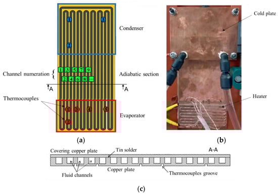
Figure 1.
FPPHP channels layout, with reference to the thermocouples location (circles) and channel numeration (squares) (a); rear side of the FPPHP (b); A-A cross section (c).
The evaporator temperature was monitored by means of five T-type thermocouples (Figure 1a) directly attached on the FPPHP surface, while the condenser temperature was acquired through three T-type thermocouples on the rear surface of the cold plate. The thermocouples’ location at the evaporator was chosen with the aim of achieving a satisfactorily uniform assessment of temperature referred to each heating section over its whole extension, without unnecessarily increasing the complexity of the manufacturing process. Given the high thermal conductivity of the adopted manufacturing material, a limited number of thermocouples at the specified locations was believed to provide reliable evaporator temperature measurements, especially for the sake of the device thermal characterization, which is based on an average value of evaporator temperature (computed over a long time-span) rather than on punctual temperature values. The ambient temperature was measured by one T-type thermocouple. The thermocouples signals were sampled at 1 Hz.
In addition, the front side surface of the device was coated with a highly emissive paint (ε = 0.92 ± 0.01) to allow measurements of the outer wall temperature within the adiabatic section by a medium wave infrared (MWIR) camera (FLIR® SC5500, sampling frequency: 50 Hz, pixel resolution: 320 × 256). The opaque paint emissivity, along with its uncertainty, was empirically estimated by performing dedicated IR acquisitions on a coated isothermal surface (same opaque paint, at controlled temperature and monitored through thermocouples). The emissivity parameter set in the IR camera software (Altair©, version 5.91.010, FLIR, Wilsonville, OR, USA) was adjusted until a match between the temperature measured by thermocouples and the one by the infrared camera was reached in the range of uncertainty of the camera (±1 °C), resulting in an emissivity of 0.92 ± 0.01. The estimated value is in accordance with the emissivity of longer waves of most opaque, commercial paints [29]. Since the emissive layer had a thickness lower than 100 μm, its thermal resistance was considered as negligible, thus reasonably assuming with that the temperature measured on top of the coating corresponded to the temperature of the device surface. In particular, the adiabatic section was framed over a 40 mm wide portion (green window in Figure 2a).
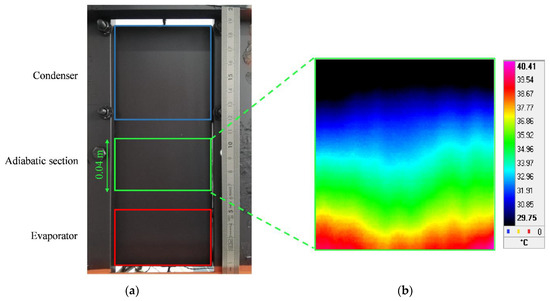
Figure 2.
Coated front side of the device, with reference to the section framed during the IR analysis (green box) (a); representative IR frame (b).
For visualization purposes, no insulation was adopted along the adiabatic section. For the same reason, both the evaporator and the condenser front surfaces were not thermally insulated, while the rear surface of the evaporator was covered with insulating material to reduce heat losses to the environment and obtain an accurate value of the actual heating power.
The uncertainty related to the experimental tools are listed in Table 1.

Table 1.
Uncertainty of the experimental equipment.
The device was first evacuated, and leak tests were performed with an ultra-high vacuum system (ASM 142, Adixen by Pfeiffer Vacuum®) and a helium detector. The FPPHP was therefore charged with a water–ethanol mixture (20 wt.% of ethanol, filling ratio: 50%), degassed by repeatedly heating and cooling the fluid in a dedicated tank. The FPPHP was positioned in vertical bottom-heat mode (BHM, evaporator below the condenser) and horizontal orientations, while the condenser temperature was fixed at 20 °C. The heat load given to the evaporator was stepwise increased from 50 W up to a maximum of 250 W due to safety reasons linked to the used materials and sensors. Some IR acquisitions, each lasting 20 s, were performed during the so-called pseudo-steady state of the device, i.e., after about 30 min from every power step applied to the evaporator. In Figure 2b, a sample of IR acquisition is shown (one single frame). The thermocouples signals were instead constantly recorded during the tests. When performing IR acquisitions, the effects of IR radiations coming from the environment and partially reflected by the surface of interest (belonging to the coated adiabatic section of the device) were considered as negligible, i.e., they did not substantially affect the IR measurements. This reasonable assumption is supported by the fact that, during the tests, the device wall temperature was at least 13 °C higher than the environmental one, and the adopted opaque coating was poorly reflective.
The IR camera settings used during the tests are reported in Table 2.
Table 2.
Camera settings.
3. Local Heat Flux Estimation Procedure
The heat flux locally exchanged at the fluid–wall interface was estimated by using the acquired IR temperature maps as inputs for the IHCP resolution approach. For the data processing, each FPPHP branch in the adiabatic section was considered as a plane-symmetric geometry (Figure 3a) due to the same boundary conditions on both outer surfaces of the device (free convection coupled with radiation). In the present analysis, the only channel walls having thickness s = xext − xint = 0.5 mm were considered (red dashed lines in Figure 3a) to better understand the heat transfer phenomena involving internal interactions between the working fluid and the device wall.
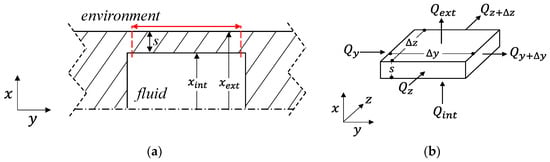
Figure 3.
Cross-sectional view of a generic FPPHP channel within the adiabatic section (a) and three-dimensional generic wall element (b).
For such a thin wall element (Figure 3b), the transient energy balance equation without heat generation reads as:
where k, ρ and cp are the solid wall thermal conductivity, density and specific heat, respectively. The boundary conditions for Equation (1), applied on the inner and outer surfaces of the channel, are, respectively, defined by Equations (2) and (3).
Here, Tenv is the room temperature and henv is the overall heat transfer coefficient between the channel wall and the surrounding environment by both natural convection and radiation. The thermal conductivity k of copper was certified equal to 401 W/mK at 20 °C and the heat transfer coefficient henv was considered equal to 10 W/m2K. The temperature at x = xint was assumed to be equal to that at x = xext (thin-wall approximation), thus simplifying the three-dimensional solid domain as a bidimensional one, where the temperature is considered to vary only along the y and z coordinates, as well as over time. By considering the infinitesimal wall section of Figure 3b with dimensions Δy and Δz, Equation (1) assumes the following formulation:
The power terms in Equation (4) are expressed as:
When Equations (5)–(8) are substituted in Equation (4), the wall-to-fluid heat flux q reads as:
During the experiments, Tenv varied from 18° C to 21 °C. For the cases under investigation, the term henv(T − Tenv) was negligible with respect to the other heat transfer terms appearing in Equation (9), thus proving that the value assumed by the overall heat transfer coefficient henv does not play a significant role in the present wall-to-fluid heat flux evaluation. By employing a sensitivity analysis on Equation (9), the term was assessed to be three orders of magnitude higher than the term, especially during the device operation. In fact, the onset of fluid motion guarantees a lower wall temperature of the whole adiabatic section, coupled with higher time–space temperature variations, drastically diminishing the relative weight of outer free convection in terms of estimation. Equation (9) can be numerically solved by approximating derivatives of temperature with finite differences. However, since noise is intrinsically present in raw experimental temperatures, Equation (9) gives unstable results, especially due to the presence of derivative operators [30]. A convenient solution to such an issue is represented by the filtering technique, a so-called regularization method employed for noise removal in inverse problems inputs [31,32,33,34]. In particular, such a regularization technique relies on the application of a Gaussian filter for high-frequency component suppression in raw data, thus fulfilling the same function of the regularization term in the Tikhonov method [35]. Nevertheless, when compared to other approaches, the filtering technique represents an effective and computationally efficient regularization method, especially when the studied physics is described by a large domain with a high number of unknown terms [36,37,38,39]. For wall temperature samples discretized into M spatial steps Δy, N spatial steps Δz and O time increments Δt, the discrete Fourier transform of the measured M × N × O temperature distribution T results in:
where u, v and w are the spatial and time coordinates in the frequency domain. By adopting the three-dimensional Gaussian filter, the Fourier image of the filtered temperature Tf is defined as:
H(u,v,w) is the transfer function for the Gaussian filter, defined as:
where uc and uw are the cut-off frequencies referred to space and time, respectively. In particular, two different cut-off frequencies were introduced since the physics of the problem could significantly vary from space to time in terms of frequency response. Moreover, a single cut-off frequency in space was considered since both spatial coordinates were believed to present similar signal-to-noise ratio due to the behavior of the IR camera sensor in space. Last, the Fourier image is converted back to the time–space domain:
However, the optimal cut-off frequencies to be given in Equation (12) for a good trade-off between smoothness of the filtered data and loose of meaningful frequencies are not known a priori in real cases, leading to the need of selecting a criterion for the choice of such regularization parameters. In the present analysis, the discrepancy principle [35] was implemented. According to this principle, the inverse problem solution can be considered satisfactorily correct if the deviation between the measured and filtered temperatures is equal to the standard deviation of the raw measurements [39,40]. In other terms, the condition to be satisfied is the following:
where ‖ ‖2 stands for the 2-norm, N·M·O is the overall size of T and σT is the time–space standard deviation of the raw data, estimated by measuring the wall temperature distribution in isothermal conditions. Specifically, Equation (14) is represented by the following minimization problem:
Nonetheless, the minimization problem of Equation (15)—required to find the optimal regularization parameters for the Gaussian filter—may not exhibit a unique solution, i.e., Equation (15) is inherently ill-posed from a mathematical standpoint. To properly estimate the optimal parameters during space and time regularizations of the data, different approaches or assumptions have been proposed in the literature. Blanc et al. [41] employed the function specification method for the space–time heat flux estimation in a cylindrical channel. A bidimensional IHCP problem in transient conditions was considered. The two physics were treated separately: the temporal stabilization parameters were assessed by identifying the time instant at which the width of rate of representation [42] exhibited a slow increase for a single temperature sensor. A physical criterion, specifically designed for the studied application, was thus adopted. On the other hand, the spatial stabilization parameters were estimated in [41] by smoothing the spatial temperature fluctuations of a desired quantity. Najafi et al. [43] used the Tikhonov method as a regularization technique for the heat flux estimation in a metallic plate partially heated from one side under transient conditions. Again, space and time were treated separately, while the two optimal regularization parameters were here estimated by minimizing the RMS error between evaluated values and exact values of heat fluxes.
Hence, in transient, bidimensional problems, the choice of optimal regularization parameters is strongly dependent on the specific study case. In the present work, another approach was proposed: a relationship between the two space–time regularization parameters was introduced by Equation (16), so that the number of independent variables in Equation (15) was reduced to one, and the uniqueness of the minimization problem solution was satisfied.
To determine the value of , two auxiliary minimization problems are defined in Equations (17) and (18), varying one parameter at a time, while tending the other to infinity. In other words, the filter is first applied to space only in Equation (17), and therefore to time only in Equation (18), thus treating the two physics separately as in previous works [41,43].
Finally, is calculated dividing uc,opt by wc,opt; the new definition for the transfer function of Equation (12) reads as:
while Equation (15) reduces to , being the only cut-off frequency to be optimized for the final 3D Gaussian filter application. For the considered experimental case, σT was evaluated in situ through IR acquisitions on the coated device under isothermal conditions (at known temperature of about 30 °C), and it was found equal to 0.04 K. Specifically, σT takes into account non-uniformities of the highly emissive coating, as well as imperfect flatness of the device outer surface, which could lead to non-physical, local temperature variations. In addition, was independently evaluated for every test condition and found in between 0.8 and 1.1 for low and high heat loads provided to the evaporator, respectively.
4. Validation of the Estimation Procedure
A dedicated validation of the estimation method by means of synthetic temperature data has been performed. The validation of the inverse procedure for the wall-to-fluid heat flux evaluation is based on four different steps [44]:
- Direct problem implementation. The heat transfer by conduction through the studied solid domain is simulated on a CFD environment by providing a known heat flux distribution qexact as a boundary condition at the wall-fluid interfaces;
- Simulation of experimental data acquisition. The resulting synthetic temperature distribution is randomly spoiled with Gaussian noise levels σ;
- Inverse problem implementation. The causal factor (imposed heat flux) that produces the given set of synthetic, experimental observations (noisy temperature distribution on the outer wall surface) is estimated. To this aim, the three-dimensional noisy temperature, being a function of the two space coordinates and time, is filtered by means of Equation (19) and used as input for Equation (9), thus attempting to evaluate back the given wall-to-fluid heat flux qexact. In particular, since the considered inverse problem concerning transient heat conduction in the bidimensional domain is intrinsically ill-posed from a mathematical standpoint (due to the presence of noise in the input temperature data which undermine the stability of the solution), Equation (19) is employed as a regularization method by filtering out the undesired noise;
- Evaluation of the estimation error. qexact is finally compared with the heat flux evaluated in step (3), qrestored, thus assessing the goodness of the estimation procedure for the given heat flux distribution and noise levels.
Step (1) was performed through the Comsol Multiphysics© software (version 5.6, COMSOL Inc., Stockholm, Sweden) by the finite elements method. More than 150,000 elements were found to guarantee the grid-independency of the model. To ensure the reliability of the method validation, the qexact given in step (1) has to be as similar as possible to the thermofluidic interactions occurring in the real device. Hence, according to the expected physical behavior in experimental cases [3,18], the convective heat flux is assumed to exhibit a sinusoidal shape described by time–space variations, representative of the working fluid oscillations through the adiabatic section:
where H is the length of the considered portion of the adiabatic section, f is the oscillation frequency of the sinusoidal signal and z is the axial coordinate. Here, variations over the z coordinate are expressed by the term , while variations over y are introduced by means of the phase φ. Adjacent channels are assumed to exhibit a phase shift equal to π. In fact, in the real FPPHP device, when hot fluid flows from the evaporator to the condenser in one channel, cold fluid is expected to flow back to the evaporator in the adjacent branches. This may result, for fixed time instants, in positive wall-to-fluid heat flux peaks in one channel (hot fluid warming up the device wall), and negative wall-to-fluid heat flux peaks (device wall cooled down by cold fluid) in the adjacent branches.
In addition, the wall-to-fluid heat flux is expected to vary between the thin walls and side walls surfaces A and B, respectively, highlighted in Figure 4 for a generic channel, thus leading to the following definition of qexact,B:
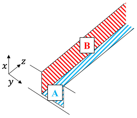
Figure 4.
Two surfaces at which qexact is defined for the generic device channel. A: thin wall; B: side wall.
Specifically, the heat flux exchanged over surface B is believed to present greater heat flux amplitudes due to the higher thermal inertia of the side walls; a validation of this assumption by preliminary experimental data will be provided at the end of the present Section.
The capability of the inverse procedure of effectively evaluating the wall-to-fluid heat flux was quantified by adopting different amplitudes and oscillation frequencies of qexact. In particular, Amp was considered equal to 2000, 4000 and 8000 W/m2K, while f was considered equal to 0.5, 0.8 and 1.2 Hz. From the direct problem simulation, the maximum residual between the inner and outer wall temperatures, i.e., for T(x = xint) and T(x = xext) according to Figure 2b, was found to be less than 0.02 K. Since such a value was lower than the noise level evaluated in Section 3 for the present experimental set-up (0.04 K), the thin-wall approximation was consequently verified.
For step (2) of the validation procedure, three different noise levels σ were adopted, namely 0.01, 0.04 and 0.08 K. To provide references for the restoration procedure of the given exact wall-to-fluid heat flux distributions, the validation data referred to two different qexact cases for a single channel ( = 0) are shown in Figure 5 by considering σ = 0.04 K and the axial coordinate z = 0.02 m.
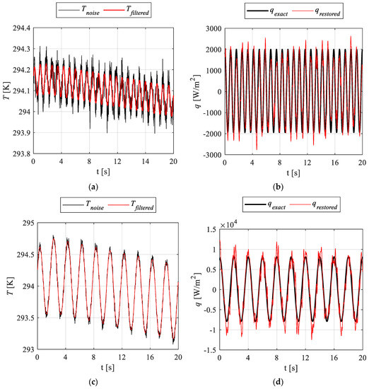
Figure 5.
Noisy and filtered temperature signals (σ = 0.04 K, z = 0.02 m) for Amp = 2000 W/m2, f = 1.2 Hz (a), and Amp = 8000 W/m2, f = 0.5 Hz (b), and corresponding exact and restored heat fluxes (c,d), respectively. The fixed axial coordinate z = 0.02 m is considered.
In Figure 5a–c, the noisy temperature Tnoise, resulting from step (2), and the filtered temperature Tfiltered, resulting from step (3), are reported for Amp = 2000 W/m2, f = 1.2 Hz and Amp = 8000 W/m2, f = 0.5 Hz, respectively. In Figure 5b–d, the exact and restored heat fluxes are additionally shown for the same test cases. In Figure 5a, the lower amplitude of the considered qexact results in lower temperature variations and lower signal-to-noise ratio, leading to a hard restoration of the exact heat flux peaks (Figure 5b) [33]. On the contrary, the heat flux of Figure 5d is restored with slightly greater accuracy thanks to the higher signal-to-noise ratio of Tnoise (Figure 5c), even though some variations from the exact value are still appreciable due to residual noise in the Tfiltered signal.
Moreover, the goodness of the assumption of Equation (21) was verified by comparing preliminary experimental data with numerical data obtained by the heat flux restoration procedure on synthetic distributions. In Figure 6, all the terms appearing in Equation (9) are plotted as a function of time for a generic PHP channel and a median axial coordinate. Specifically, , , and . In other words, qz, qy and qt are the terms constituting the inverse solution, while qA and qB in Equation (21) are the parameters used in the direct problem for the generation of synthetic data. Specifically, the amplitude of the heat flux exchanged on the B surface may influence the terms of the heat flux exchanged on the thin-wall surface due to a redistribution of temperature by conduction in the solid domain. Hence, qz, qy and qt were considered in both the numerical and the experimental cases to better understand the relationship between qA and qB, and to qualitatively assess the reasonability of the assumption of Equation (21). Figure 6a refers to the numerical data, while Figure 6b refers to the preliminary experimental data. From the restoration procedure on synthetic data (Figure 6a), obtained by adopting Equation (21), the peaks assume values about half, in module, of those assumed by , while approaches the positive peaks of . A comparable behavior can be perceived from the heat flux evaluation on the preliminary data (Figure 6b), at least when stable (nearly sinusoidal) oscillations occur (until 12 s), thus confirming the assumption of Equation (21). Figure 6a,b are not here intended to be quantitatively compared in a rigorous way, since the exact wall-to-fluid heat flux (sinusoidal function) used to generate synthetic data clearly differs from the one exchanged in the real device, which is undoubtedly subjected to more complex thermofluidic interactions.
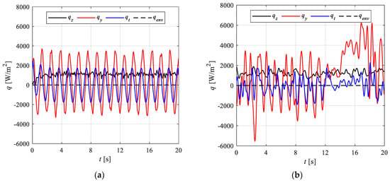
Figure 6.
Comparison between numerical (a) and experimental (b) data for the validation of the assumption adopted in Equation (21).
Finally, the restoration error for step (4) was defined as:
Since the effectiveness of the Gaussian kernel is dependent on the randomly generated noise distribution of step (2), steps (2–4) were repeated for 100 different random sequences of noise to the numerical data and an averaged value of E was evaluated for each considered noise level.
The estimation error, evaluated for every combination of frequency and amplitude of , and for every considered noise level, is reported in Table 3. Here, the restoration error E generally decreases with the increase of Amp, while it increases with f, as is already highlighted for bidimensional approaches [27]. For a noise level equal to 0.04 K (present experimental set-up), the estimation error was found in the range 11% to 15% of , thus validating the rather good accuracy of the wall-to-fluid heat flux evaluation procedure of Section 3. It must be highlighted that the assessed estimation error is in accordance with the ones found in other studies concerning IHPC resolution approaches by means of the filtering technique as a regularization method [27,32,37,39]. Its relatively high value has to be accounted for the smoothing performed by the Gaussian filter on the high amplitude peaks in the input data. Nonetheless, its adoption leads to fast and reliable post-processing, satisfactorily allowing a quantification of wall-to-fluid heat fluxes exchanged in the device under investigation.
Table 3.
Restoration error E as a function of noise level σ, for different amplitudes of qexact and frequencies f.
5. Results and Discussion
5.1. Global Performance Evaluation
The device was first characterized, for every considered study case, by evaluating its global performance, which is the most employed figure of merit in the description of PHPs [3]. Hence, the equivalent thermal resistance was quantified by means of the following definition:
where and are the evaporator and condenser temperatures, respectively, averaged over 5 min during the pseudo-steady state of the FPPHP, and is the net power input provided to the evaporator. Since part of the evaporator section was not insulated, was quantified as , where is the power dissipated at the evaporator section to the environment by free convection and radiation. The non-insulated evaporator surface was estimated, according to the FPPHP geometry, equal to 0.0037 m2. The maximum dissipated power of about 1.4 W was found for the most critical case in terms of device operation, such as the horizontal orientation, Q = 250 W, where the evaporator exhibited an average temperature of 50 °C. During the tests, the environmental temperature ranged from about 18 °C to 21 °C.
Moreover, the uncertainty , referred to each value of , was evaluated by means of the approach by Kline and McClintock [45]:
where is the uncertainty referring to ) and is the uncertainty on the net heat load, which depends on the uncertainty of the power supply (Table 1).
In Figure 7, the resulting evaluated by means of Equation (23) is shown for each net heat load and configuration, together with the corresponding error bars. The equivalent thermal resistance for the empty device was assessed to be almost equal to 0.7 K/W. In particular, the empty device was tested by adopting the same experimental set-up described in Section 2 (although the device was not here filled with working fluid after the vacuuming procedure). In fact, comparing the thermal performance of the partially filled device with the empty one through the same experimental apparatus is a rather standard procedure in the PHP field, which discloses the thermal advantages of using a certain amount of working fluid for a given PHP geometry [3,11,18]. Heat loads of 50, 100 and 150 W were, respectively, provided to the evaporator. As expected, the equivalent thermal resistance of the empty device (filling ratio = 0%) was higher than that of the device partially filled with fluid (filling ratio = 50%). Moreover, Req did not change from heat load to heat load, since heat transfer between the evaporator and the condenser was here solely due to conduction through the metallic walls.
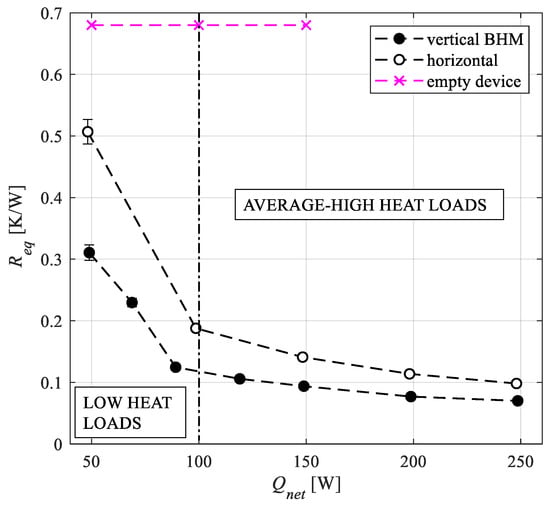
Figure 7.
Equivalent thermal resistances of the studied FPPHP.
It has to be pointed out that “low heat loads” and “average-high heat loads” in Figure 7 are expressions whose meaningfulness is only related to the operational limits of the device under investigation. The maximum power input of 250 W was set as safety threshold for the experimental equipment, even though the device could have endured even higher power inputs before the onset of a full dry-out at the evaporator section (i.e., before the FPPHP failure). Hence, power inputs lower than 100 W are here referred as “low”, while higher power inputs are referred as “average-high”. For every heat load, the vertical BHM presents lower values of with respect to the horizontal orientation, denoting better thermal performances within the gravity-assisted mode in agreement with Ayel et al. [28]. In addition, for both configurations, strongly decreases until about = 100 W, to approach an almost asymptotic value at high power inputs. Such abrupt change in trend is because the device experiences a significant variation in terms of working behavior from low power inputs ( < 100 W) to higher heat loads. Specifically, for < 100 W, intermittent flows occur (i.e., flows characterized by frequent stopovers which undermine the device performance), while, at high power inputs, the device is fully activated (i.e., the fluid regularly flows in every channel, ensuring a proper and constant heat dissipation to the condenser). Such a transition in terms of working regime is due to stronger phase-change phenomena at the evaporator, which could not be regularly sustained at power inputs lower than 100 W. In fact, a relevant part of the provided heat loads was transferred to the condenser by conduction through the copper walls of the device, i.e., the dissipated heat did not take part in fluid evaporation.
5.2. Local Heat-Transfer
To present a deep overview of the device heat transfer behavior, the wall-to-fluid heat flux q was evaluated for every study case by adopting the post-processing procedure described in Section 3. It has to be reminded that q is not here referred to the whole wall-fluid interface, but only to the median portion of thin walls in each channel (Figure 3a). However, despite such an evaluated thermal quantity it is limited to the thermofluidic interactions within a rather small part of the device, it is believed to describe the FPPHP thermal behavior in terms of fluid oscillations and working regimes. In fact, the low thickness of such a portion guarantees higher wall temperature variations, directly linked to the inner thermo-dynamics.
In Figure 8, the raw temperature acquired by means of thermography is shown (Figure 8a), together with the corresponding assessed wall-to-fluid heat flux distribution (Figure 8b) for a single test case (horizontal orientation and Q = 50 W) and for channel 8 (central channel, see reference of Figure 1a). Both quantities are additionally plotted in Figure 9 and Figure 10 for Q = 100 W and Q = 200 W, respectively, and for the same orientation and reference channel.
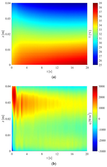
Figure 8.
Space–time temperature distribution acquired by means of thermography (a) and resulting wall-to-fluid heat flux q (b); (channel 8, horizontal orientation, Q = 50 W).
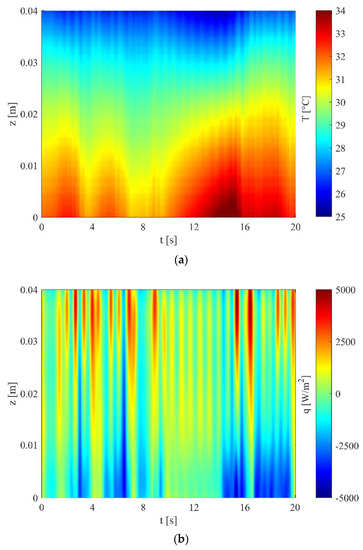
Figure 9.
Space–time temperature distribution acquired by means of thermography (a) and resulting wall-to-fluid heat flux q (b); (channel 8, horizontal orientation, Q = 100 W).
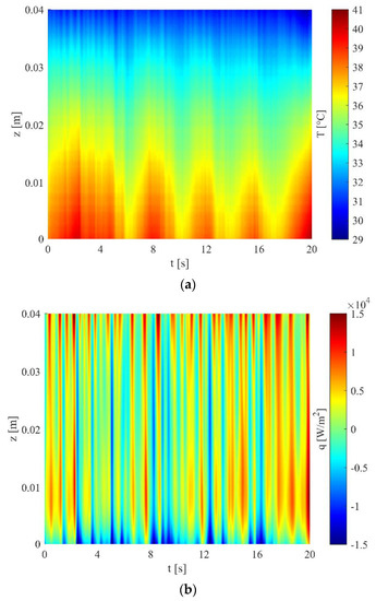
Figure 10.
Space–time temperature distribution acquired by means of thermography (a) and resulting wall-to-fluid heat flux q (b); (channel 8, horizontal orientation, Q = 200 W).
According to the adopted reference system (Figure 3), the wall-to-fluid heat flux is positive when it is exchanged by the working fluid to the device wall, i.e., the wall heats up. Hence, fluid motion can be perceived and described in most of the cases as follows:
- When the wall-to-fluid heat flux significantly increases over time, hot fluid may flow from the evaporator to the condenser, thus warming up the wall;
- When the wall-to-fluid heat flux significantly decreases over time, flow reversal phenomena may occur, where fluid colder than the wall flows back from the condenser to the evaporator.
During the intermittent flow (Figure 8), the temperature distribution does not exhibit substantial variations over time except for the first seconds, in which few temperature fluctuations can be perceived. Similarly, the wall-to-fluid heat flux (Figure 8b) does not vary over the whole observation window but only the first few seconds, confirming an almost constant absence of fluid motion. As long as the power input to the evaporator increases, variations of both temperature and heat flux become more and more persistent over time, verifying the onset of a device full activation. The oscillatory behavior of the studied FPPHP is thus clearly noticeable from the alternation of peaks, either positive or negative, in the wall-to-fluid heat flux distribution of Figure 9b and Figure 10b: straight vertical peaks suggest that the working fluid flows almost instantaneously, i.e., at high velocity, through the analyzed channel for both considered heat loads. It has to be pointed out that the amplitude of q presents non-negligible variations along the z coordinate. In particular, the wall-to-fluid heat flux exhibits, in all the reported study cases, an increasing trend from the evaporator (z < 0 m), where it seems to assume lower values, to the condenser (z > 0.04 m), where it seems to assume higher values instead. Such variations are especially notable at low and intermediate power inputs (Figure 8 and Figure 9), while, for high power inputs (Figure 10), amplitudes of the wall-to-fluid heat flux are more uniform along space. To better outline heat flux variations along space, the values of q, averaged over time (qav), are shown in Figure 11 as a function of the axial coordinate z for three FPPPHP branches, namely channels 3, 10 and 16, and the representative test case of Figure 9 (horizontal, 100 W). Specifically, two outer channels and one middle channel were chosen as meaningful branches. Here, the wall-to-fluid heat flux clearly exhibits an increasing trend with z in all the considered channels, thus verifying the presence of significant space variations in the heat flux distributions. Such a characteristic local heat transfer behavior might be due to the conductive heat transfer in the thick wall between the evaporator and the condenser, which propagates to the section of interest (adiabatic section) the effects of both heat transfer areas on the working fluid.
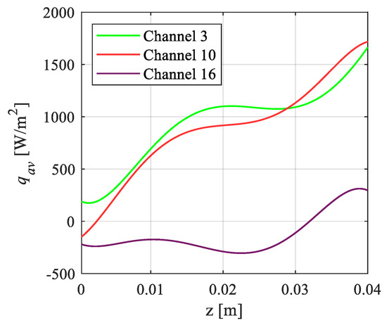
Figure 11.
Wall-to-fluid heat flux averaged over time, as a function of the axial coordinate for three meaningful channels (horizontal orientation, Q = 100 W).
It has to be considered that the observed variation of q along the axial coordinate depends on the geometry and the material of the studied device, which is highly conductive. On the contrary, by considering different kinds of materials, e.g., polymeric materials, or different geometries, e.g., tubular layouts, the wall-to-fluid heat flux distributions could present negligible space variations, as stated in [27] and [46].
5.3. Quantitative Description of the Local Heat Flux Variations
To achieve a quantitative and repeatable description of channel-wise heat flux variations, two coefficients of variation, namely cvt (over time) and cvs (along space), were introduced and evaluated by means of Equations (25) and (26). Due to the high number of available data provided by the method of Section 3, such quantities were adopted to statistically reduce the wall-to-fluid heat flux distributions, as suggested in [27] and [46] for different types of PHPs. In Equations (25) and (26), the std and mean operators are the standard deviation and the arithmetic mean, respectively, N is the total number of considered axial coordinates (140), M are the considered time instants (1000) and qn is the wall-to-fluid heat flux distribution related to the n-th channel.
The use of the average in Equations (25) and (26) is due to the fact that, from a statistical point of view, a specific time–space coordinate, i.e., a single pair of i and t, is not representative of the actual variation of the time–space heat flux distributions. In particular, the statistical coefficient cvtn describes the irregularity of heat flux variations in each FPPHP channel over time: for elevated cvtn values, the fluid oscillations are regarded as strongly irregular, denoting the presence of stopovers during the observation window. On the contrary, a low cvtn denotes fluid oscillations which are substantially regular and persistent in terms of amplitude over time. To provide an order of magnitude for the regularity of thermofluidic interactions quantified by cvtn, sine-shaped functions (highest regularity) present coefficient of variation equal to about 50%, whereas constant functions are characterized by coefficient of variation of 0%. Other complementary remarks can be obtained by cvsn: high values of such a quantity denote great variations of the heat flux from end to end of the channel, while low values suggest that the entire channel is simultaneously interested by the same heat transfer phenomenon. To give a better thermal description of the overall device, the average and the standard deviation of cvtn and cvsn, denoted by the subscript av and std, respectively, were computed by considering all the analyzed FPPHP channels num as follows:
where cv is the generic coefficient of variation (either over time or along space). The coefficient of Equation (27) describes the average heat flux variation either over time (cvtav) or along space (cvsn) in the entire adiabatic section of the device. The coefficient of Equation (28) quantifies instead time (cvtstd) and space (cvsstd) variations of the estimated heat flux from channel to channel. It has to be stressed that these parameters offer a critical evaluation of the goodness of numerical codes, since they represent the real statistical behavior of the FPPHP.
5.3.1. Heat Flux Variation over Time
As already pointed out in Section 5.2, fluctuations over time of the local wall-to-fluid heat flux are able to describe the fluid oscillatory flow through the adiabatic section. Hence, the device performance, which is linked to its fluid dynamics, is believed to be strictly dependent on the local heat transfer interactions. To investigate such an interplay between global and local thermal behaviors, the values assumed by q over time in every FPPHP branch for a single axial coordinate, namely z = 0.02 m, were carefully investigated.
In Figure 12, q is shown for two different operating conditions, i.e., horizontal orientation, Q = 50 W (Figure 12a), and vertical BHM orientation, Q = 150 W (Figure 12b); three representative channels are considered. In the horizontal configuration (Figure 12a), during the first 2 s of acquisition, the heat flux oscillates in every analyzed channel, suggesting fluid motion between the evaporator and the condenser, while it starts approaching null values after 2 s without any significant oscillation, denoting instead absence of fluid motion. On the contrary, in the vertical BHM operation (Figure 12b), q presents regular and persistent oscillations for every PHP branch, i.e., the fluid is regularly flowing in the overall adiabatic section.
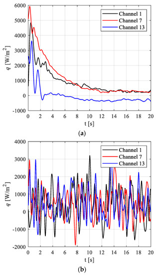
Figure 12.
Local heat fluxes referred to every channel for the horizontal orientation at Q = 50 W (a) and for the vertical BHM at Q = 150 W (b).
The heat flux variations over time were therefore statistically investigated by means of cvt to provide a quantitative description of fluid oscillations from intermittent flows to full activations. In Figure 13, cvtav and cvtstd are shown for the two considered orientations as functions of the power input to the evaporator. For heat loads lower than 100 W, cvtav reaches peaks of about 75%, while cvtstd decreases to about 10%. At average-high heat loads, cvtav and cvtstd stabilize around 70% and 8% for both orientations, thus giving a further reference for the description of the significant change in slope of Req from intermittent flow to full activation of the device (Figure 7). The provided values and general trends of the statistical coefficients are in good agreement with those found in [46] for a tubular layout, although the very different geometry analyzed in the present work, suggesting the validity of the adopted statistical coefficients for other PHPs layouts.
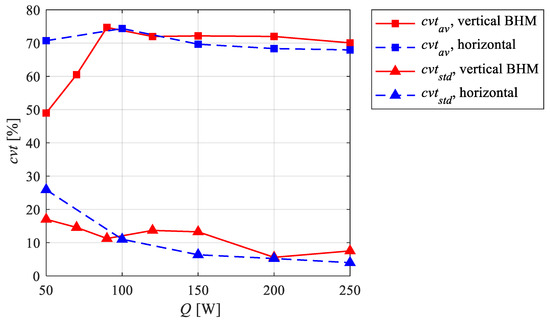
Figure 13.
cvtav and cvtstd, as functions of the heat load, for the two considered orientations.
Furthermore, the intermittent flow regime in the horizontal orientation, when compared to the vertical BHM orientation, exhibits, at 50 W, higher values of cvtav and cvtstd. This suggests stronger variations over time of the heat flux from channel to channel and, consequently, a more intermittent operation of the FPPHP, in accordance with previous works [47,48,49]. Additionally, such evidence agrees with the higher value of equivalent thermal resistance observed in Figure 7. On the other hand, within the full activation of the system, cvtav and cvtstd assume similar values for both orientations, highlighting comparable heat flux variations over time. Such similarity may explain the gradual approaching of equivalent thermal resistance referred to both orientations at elevated heat loads to the evaporator.
5.3.2. Heat Flux Variations over Space (z Coordinate)
As observed in Section 5.2, space variations of the wall-to-fluid heat flux are clearly noticeable in the adiabatic section of the present FPPHP, probably due to the conductive thermal interactions between the adiabatic section and the evaporator/condenser. To give a better insight into these local heat flux variations along space, cvs was analyzed alike cvt.
In Figure 14, cvsav and cvsstd are shown for the two considered orientations. Here, cvsav referring to both the vertical BHM orientation and the horizontal orientation decreases at low power inputs, to settle around 43% and 50%, respectively, at average-high power inputs. In addition, cvsstd decreases almost monotonically from a maximum of about 20% to a minimum of about 8% for both orientations. Such trends denote that the variations over space tend to gradually decrease during the intermittent flow regime in the overall device unlike time variations of Figure 13, while they stabilize during the full activation regime. Such a remark suggests that the conduction effects through the metallic section of the present FPPHP are evident in both orientations especially during the intermittent flow regime, where the unregular operation of each FPPHP branch promotes the onset of strong conduction along the z coordinate, as stated in [18]. On the other hand, the stabilization of cvsav at lower values during the full activation regime denotes less predominant conduction effects, confirming what was qualitatively observed in Section 5.2. Moreover, the higher values assumed by cvsav in the horizontal operation with respect to those assumed in the vertical BHM suggest that the wall-to-fluid interactions are distributed in a less uniform way along the z coordinate, probably due to weaker fluid oscillations. Finally, the values of cvs in the present FPPHP assume much higher values with respect to those previously assessed for a tubular layout [46], where the conduction through the adiabatic section was almost negligible, thus confirming the presence of strong conductive phenomena occurring in the studied FPPHP geometry.
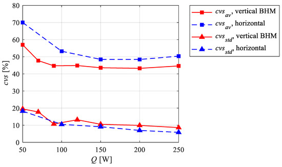
Figure 14.
cvsav and cvsstd, as functions of the heat load for the two considered orientations.
To provide a reference for the understanding of conduction between the evaporator and the condenser at varying heat loads in the present FPPHP, the ratio between the power transferred only by conduction through the copper plate and the net power input given to the evaporator is shown in Figure 15. Specifically, using the values of evaporator and condenser temperature averaged over 5 min during the pseudo-steady state for each given heat load results in:
where is the full metallic cross-section of the device and is the length of the adiabatic section. is the device thickness, is the device total width, is the side dimension of channels and num is the total number of channels.
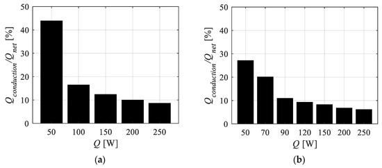
Figure 15.
Ratio between the power transferred by conduction between the evaporator and the condenser and the net power input to the evaporator as a function of power input for the horizontal orientation (a) and the vertical BHM (b).
For both orientations, decreases with respect to the net power input, suggesting that more and more power provided to the evaporator is transferred by the working fluid to the condenser from the intermittent flow to the full activation regime. Hence, this confirms the reduction in terms of heat flux variations over space within the adiabatic section, quantified in Figure 14, as well as the different values assumed by cvsav from horizontal orientation to vertical BHM.
5.4. Statistical Amplitude of the Local Heat Flux
In Section 5.3, time–space fluctuations of the local wall-to-fluid heat flux distributions (referred to each power step provided to the evaporator) were representative of the FPPHP working regimes and linked to the device global performance. However, the amplitude of q, which could be of great interest for the improvement of existing numerical models of FPPHPs, is not yet properly investigated. Hence, to provide additional quantitative information regarding the local thermal interactions occurring within the adiabatic section in the median section of each device branch, the wall-to-fluid amplitude was statistically reduced for every test case. In particular, the 80th percentile of the absolute value of q, q80, was chosen as a representative statistical parameter for the given set of data since it was proven to successfully catch the amplitude of local thermofluidic interactions by neglecting non-statistical high peaks of the wall-to-fluid heat flux [50].
In Figure 16, q80 is plotted as a function of Q: here, strong wall-to-fluid thermal interactions can be noted in the horizontal orientation, where q80 increases from 1000 W/m2 to about 7100 W/m2. On the contrary, in the vertical BHM orientation, q80 slightly increases from 1000 W/m2 to about only 2200 W/m2. Such a significant difference in terms of amplitude, which was also perceived in a tubular layout [46], is merely due to the effects of the device orientation. In fact, in the vertical BHM operation, the buoyancy forces greatly promote the fluid motion inside the device, resulting in a lower pressure (and, consequently, lower saturation temperature) needed for the working fluid motion and more regular temperature distribution along the channels. Hence, weaker temperature differences between the FPPHP wall and the working fluid are generally perceivable, leading to lower wall-to-fluid heat fluxes.
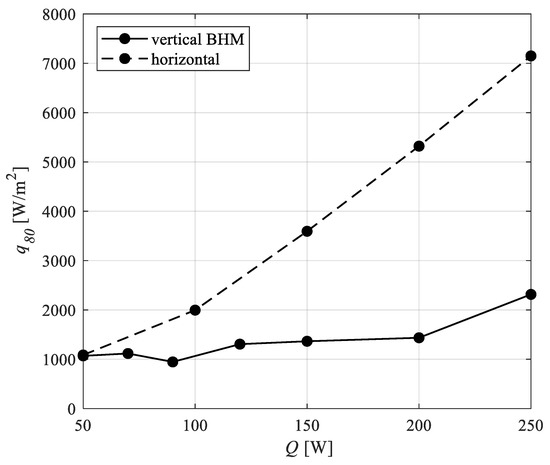
Figure 16.
80th percentile of the absolute value of q as a function of the heat load to the evaporator for the two considered orientations.
6. Conclusions
A metallic FPPHP with a total of 16 channels (8 turns in the evaporator zone) was experimentally studied in vertical BHM and horizontal orientation to assess its local thermal behavior at heat loads ranging from 50 to 250 W. The adopted operating fluid was a water–ethanol mixture, with volumetric filling ratio of 50%. The evaporator/condenser temperature was monitored by thermocouples, thus allowing device characterization by evaluating its equivalent thermal resistance. The external wall temperature in the adiabatic zone was acquired by means of an IR camera. The resulting time–space temperature maps, effectively pre-processed by a three-dimensional Gaussian filtered, were used as inputs for the IHCP resolution approach for the evaluation of the heat flux exchanged between the working fluid and the thin walls of the device. The method was validated by adopting synthetic data. The wall-to-fluid heat fluxes were first statistically reduced to quantify, by means of two dedicated coefficients, namely cvt and cvs, their time and space variations from channel to channel. The analysis of these coefficients supplied a quantitative tool for the identification and description of the device working regimes. In addition, statistical heat flux amplitudes q80 were presented to achieve a comprehensive overview of the local wall-to-fluid thermal interactions. In general, as expected, the wall-to-fluid heat flux distributions exhibit a significant variation over both time and space in every channel.
The most meaningful and quantitative results of the current study are summarized as follows:
- The maximum estimation error for the adopted inverse approach was assessed equal to about 15% of the wall-to-fluid interactions occurring in the real set-up;
- In the intermittent flow (Q < 100 W), cvtav and cvtstd assume values up to around 75% and 30% for both orientations, respectively, denoting a generally discontinuous FPPHP operation. On the contrary, the two coefficients stabilize at about 70% and 8% during the device full activation (Q > 100 W), thus denoting comparable fluid oscillatory behaviors at high heat loads, which result in similar device global performances;
- cvsav decreases for both orientations within the intermittent flow to settle at around 43% and 50%, respectively, during the full activation, suggesting that the wall-to-fluid interactions are more uniformly distributed along the device axis with the onset of stable and full fluid oscillations;
- q80 reaches a maximum of 7100 W/m2 in the horizontal orientation at Q = 250 W, while it increases up to 2200 W/m2 in the vertical BHM.
In conclusion, the presented non-intrusive approach, coupled with a statistical reduction of the available data, has been proven to provide quantitative pieces of information regarding the wall-to-fluid thermal interactions and heat transfer modes of FPPHPs. The identification of the two-phase flow regimes can be carried out without the need of a transparent insert, a transparent plate or a multilayer sheet for IR analysis, and even from thermographic maps acquired on a metallic, opaque geometry. The evaluated local heat transfer quantities can be extensively used for the design of these heat transfer devices, as well as for the benchmarking of existing numerical models.
Author Contributions
Conceptualization, L.P. and F.B.; methodology, L.P., F.B. and L.C.; software, L.P.; validation, L.P. and M.S.; formal analysis, L.P. and F.B.; investigation, L.P., M.S., V.A. and C.R.; resources, F.B. and V.A.; data curation, L.P. and L.C.; writing—original draft paper, L.P.; writing—review and editing, F.B., L.C., V.A. and S.R.; visualization, L.P.; supervision, F.B., V.A. and S.R.; project administration, F.B., V.A. and C.R.; funding acquisition, F.B., V.A. and S.R. All authors have read and agreed to the published version of the manuscript.
Funding
This research was funded by the European Space Agency (ESA) grant number 4000128640/19/NL/PG/pt, ESA MAP project TOPDESS.
Institutional Review Board Statement
Not applicable.
Informed Consent Statement
Not applicable.
Data Availability Statement
The data presented in this study are available on request from the corresponding author. The data are not publicly available due to the large dataset.
Acknowledgments
The work has been carried out through a fruitful and effective collaboration between the University of Parma and the University of Poitiers. The Authors would like to acknowledge the European Space Agency (ESA) support. The Authors would also like to thank Marco Marengo for fruitful discussions.
Conflicts of Interest
The authors declare no conflict of interest.
Nomenclature
| Symbol | Quantity | SI Unit |
| Amp | Heat flux amplitude | W/m2 |
| cp | Specific heat at constant pressure | J/kg·K |
| cvt | Coefficient of variation (time) | % |
| cvtav | Mean of the coefficient of variations over the whole device | % |
| cvtstd | Standard deviation of the coefficients of variation over the whole device | % |
| E | Restoration error | % |
| f | Heat flux frequency | Hz |
| Discrete Fourier transform | - | |
| H | Transfer function (Gaussian filter) | - |
| henv | Overall heat-transfer coefficient between the channel wall and the surrounding environment by both natural convection and radiation | W/m2K |
| k | Thermal conductivity | W/m·K |
| Ladiab | Length of the adiabatic section | m |
| lchannel | Channel height | m |
| M | Number of time samples of the generic thermographic temperature distribution | - |
| N | Number of axial coordinates of the generic thermographic temperature distribution | - |
| num | Total number of channels | - |
| O | Number of y coordinates of the generic thermographic temperature distribution | |
| q | Convective heat flux per unit surface | W/m2 |
| Q | Electrical power input to the evaporator | W |
| qav | Heat flux averaged over time | W/m2 |
| Qconduction | Power transferred by conduction between evaporator and condenser | W |
| qexact | Synthetic heat flux | W/m2 |
| Qnet | Net power input to the evaporator, considering heat dissipation to the environment | W |
| qrestored | Restored synthetic heat flux | W/m2 |
| Ratio between time and space cut-off frequencies | - | |
| Renv | Overall heat-transfer resistance between the external tube wall and the surrounding environment | m2·K/W |
| Req | Equivalent thermal resistance | W/°C |
| s | Thickness of the thin-wall of the channel | m |
| Scopper | Full metallic cross-section | m2 |
| S’eva | Non-insulated evaporator outer surface | m2 |
| t | Time | s |
| T | Temperature | °C |
| Tenv | Environmental temperature | K |
| Tf | Filtered experimental temperature | K |
| TFPPHP | Device thickness | m |
| u, v, w | Frequency components | rad−1 |
| uc, wc | Cut-off frequencies | rad−1 |
| WFPPHP | Device width | m |
| xint | Half of the channel height | m |
| z | Axial coordinate | m |
| δ | Uncertainty of experimental tools | - |
| ε | Emissivity | - |
| ρ | Density | kg/m3 |
| σ | Noise level | K |
| φ | Heat flux phase | rad |
References
- Murshed, S.M.S.; de Castro, C.A.N. A critical review of traditional and emerging techniques and fluids for electronics cooling. Renew. Sustain. Energy Rev. 2017, 78, 821–833. [Google Scholar] [CrossRef]
- MMousa, H.; Yang, C.-M.; Nawaz, K.; Miljkovic, N. Review of heat transfer enhancement techniques in two-phase flows for highly efficient and sustainable cooling. Renew. Sustain. Energy Rev. 2022, 155, 111896. [Google Scholar] [CrossRef]
- VNikolayev, S.; Marengo, M. Pulsating Heat Pipes: Basics of Functioning and Modeling. In Encyclopedia of Two-Phase Heat Transfer and Flow IV; Thome, J.R., Ed.; World Scientific Publishing: Singapore, 2018; pp. 63–139. [Google Scholar] [CrossRef]
- Mangini, D.; Mameli, M.; Georgoulas, A.; Araneo, L.; Filippeschi, S.; Marengo, M. A pulsating heat pipe for space applications: Ground and microgravity experiments. Int. J. Therm. Sci. 2015, 95, 53–63. [Google Scholar] [CrossRef]
- Bastakoti, D.; Zhang, H.; Li, D.; Cai, W.; Li, F. An overview on the developing trend of pulsating heat pipe and its performance. Appl. Therm. Eng. 2018, 141, 305–332. [Google Scholar] [CrossRef]
- Mameli, M.; Besagni, G.; Bansal, P.K.; Markides, C.N. Innovations in pulsating heat pipes: From origins to future perspectives. Appl. Therm. Eng. 2022, 203, 117921. [Google Scholar] [CrossRef]
- Yang, H.; Khandekar, S.; Groll, M. Performance characteristics of pulsating heat pipes as integral thermal spreaders. Int. J. Therm. Sci. 2009, 48, 815–824. [Google Scholar] [CrossRef]
- Kim, M.; Moon, J.H. Deep neural network prediction for effective thermal conductivity and spreading thermal resistance for flat heat pipe. Int. J. Numer. Methods Heat Fluid Flow 2022. ahead-of-print. [Google Scholar] [CrossRef]
- Zhu, M.; Huang, J.; Song, M.; Hu, Y. Thermal performance of a thin flat heat pipe with grooved porous structure. Appl. Therm. Eng. 2020, 173, 115215. [Google Scholar] [CrossRef]
- Moon, J.H.; Wang, X.; Fadda, D.; Shin, D.H.; Lee, J.; You, S.M. Effect of integrated copper pad on the performance of boiling-driven wickless thermal ground plane. Appl. Therm. Eng. 2021, 199, 117595. [Google Scholar] [CrossRef]
- Ayel, V.; Araneo, L.; Scalambra, A.; Mameli, M.; Romestant, C.; Piteau, A.; Marengo, M.; Filippeschi, S.; Bertin, Y. Experimental study of a closed loop flat plate pulsating heat pipe under a varying gravity force. Int. J. Therm. Sci. 2015, 96, 23–34. [Google Scholar] [CrossRef]
- Jang, D.S.; Lee, J.S.; Ahn, J.H.; Kim, D.; Kim, Y. Flow patterns and heat transfer characteristics of flat plate pulsating heat pipes with various asymmetric and aspect ratios of the channels. Appl. Therm. Eng. 2017, 114, 211–220. [Google Scholar] [CrossRef]
- Wang, G.; Quan, Z.; Zhao, Y.; Wang, H. Performance of a flat-plate micro heat pipe at different filling ratios and working fluids. Appl. Therm. Eng. 2019, 146, 459–468. [Google Scholar] [CrossRef]
- Alijani, H.; Çetin, B.; Akkuş, Y.; Dursunkaya, Z. Effect of design and operating parameters on the thermal performance of aluminum flat grooved heat pipes. Appl. Therm. Eng. 2018, 132, 174–187. [Google Scholar] [CrossRef]
- Lee, J.; Joo, Y.; Kim, S.J. Effects of the number of turns and the inclination angle on the operating limit of micro pulsating heat pipes. Int. J. Heat Mass Transf. 2018, 124, 1172–1180. [Google Scholar] [CrossRef]
- Chang, G.; Li, Y.; Zhao, W.; Xu, Y. Performance investigation of flat-plate CLPHP with pure and binary working fluids for PEMFC cooling. Int. J. Hydrog. Energy 2021, 46, 30433–30441. [Google Scholar] [CrossRef]
- Wang, G.; Quan, Z.; Zhao, Y.; Wang, H. Effect of geometries on the heat transfer characteristics of flat-plate micro heat pipes. Appl. Therm. Eng. 2020, 180, 115796. [Google Scholar] [CrossRef]
- Ayel, V.; Slobodeniuk, M.; Bertossi, R.; Romestant, C.; Bertin, Y. Flat plate pulsating heat pipes: A review on the thermohydraulic principles, thermal performances and open issues. Appl. Therm. Eng. 2021, 197, 117200. [Google Scholar] [CrossRef]
- Majumder, A.; Mehta, B.; Khandekar, S. Local Nusselt number enhancement during gas–liquid Taylor bubble flow in a square mini-channel: An experimental study. Int. J. Therm. Sci. 2013, 66, 8–18. [Google Scholar] [CrossRef]
- Markal, B.; Candere, A.; Avci, M.; Aydin, O. Investigation of flat plate type pulsating heat pipes via flow visualization-assisted experiments: Effect of cross sectional ratio. Int. Commun. Heat Mass Transf. 2021, 125, 105289. [Google Scholar] [CrossRef]
- Kwon, G.H.; Kim, S.J. Experimental investigation on the thermal performance of a micro pulsating heat pipe with a dual-diameter channel. Int. J. Heat Mass Transf. 2015, 89, 817–828. [Google Scholar] [CrossRef]
- Kamijima, C.; Yoshimoto, Y.; Abe, Y.; Takagi, S.; Kinefuchi, I. Relating the thermal properties of a micro pulsating heat pipe to the internal flow characteristics via experiments, image recognition of flow patterns and heat transfer simulations. Int. J. Heat Mass Transf. 2020, 163, 120415. [Google Scholar] [CrossRef]
- Takawale, A.; Abraham, S.; Sielaff, A.; Mahapatra, P.S.; Pattamatta, A.; Stephan, P. A comparative study of flow regimes and thermal performance between flat plate pulsating heat pipe and capillary tube pulsating heat pipe. Appl. Therm. Eng. 2019, 149, 613–624. [Google Scholar] [CrossRef]
- Kim, J.; Kim, S.J. Experimental investigation on working fluid selection in a micro pulsating heat pipe. Energy Convers. Manag. 2020, 205, 112462. [Google Scholar] [CrossRef]
- Jo, J.; Kim, J.; Kim, S.J. Experimental investigations of heat transfer mechanisms of a pulsating heat pipe. Energy Convers. Manag. 2019, 181, 331–341. [Google Scholar] [CrossRef]
- Kim, T.H.; Kommer, E.; Dessiatoun, S.; Kim, J. Measurement of two-phase flow and heat transfer parameters using infrared thermometry. Int. J. Multiph. Flow 2012, 40, 56–67. [Google Scholar] [CrossRef][Green Version]
- Pagliarini, L.; Cattani, L.; Bozzoli, F.; Mameli, M.; Filippeschi, S.; Rainieri, S.; Marengo, M. Thermal characterization of a multi-turn pulsating heat pipe in microgravity conditions: Statistical approach to the local wall-to-fluid heat flux. Int. J. Heat Mass Transf. 2021, 169, 120930. [Google Scholar] [CrossRef]
- Ayel, V.; Slobodeniuk, M.; Bertossi, R.; Karmakar, A.; Martineau, F.; Romestant, C.; Bertin, Y.; Khandekar, S. Thermal performances of a flat-plate pulsating heat pipe tested with water, aqueous mixtures and surfactants. Int. J. Therm. Sci. 2022, 178, 107599. [Google Scholar] [CrossRef]
- Shakir, H.M.F.; Ali, A.; Zubair, U.; Zhao, T.; Rehan, Z.A.; Shahid, I. Fabrication of low emissivity paint for thermal/NIR radiation insulation for domestic applications. Energy Rep. 2022, 8, 7814–7824. [Google Scholar] [CrossRef]
- Beck, J.V.; Blackwell, B.; Clair, C.R.S., Jr. Inverse Heat Conduction: Ill-Posed Problems; John Wiley & Sons, Inc.: New York, NY, USA, 1985. [Google Scholar]
- Murio, D.A. The Mollification Method and the Numerical Solution of Ill-Posed Problems; John Wiley & Sons: New York, NY, USA, 1993. [Google Scholar]
- Delpueyo, D.; Balandraud, X.; Grédiac, M. Heat source reconstruction from noisy temperature fields using an optimised derivative Gaussian filter. Infrared Phys. Technol. 2013, 60, 312–322. [Google Scholar] [CrossRef]
- Bozzoli, F.; Pagliarini, G.; Rainieri, S. Experimental validation of the filtering technique approach applied to the restoration of the heat source field. Exp. Therm. Fluid Sci. 2013, 44, 858–867. [Google Scholar] [CrossRef]
- Rainieri, S.; Bozzoli, F.; Pagliarini, G. Characterization of an uncooled infrared thermographic system suitable for the solution of the 2-D inverse heat conduction problem. Exp. Therm. Fluid Sci. 2008, 32, 1492–1498. [Google Scholar] [CrossRef]
- Morozov, V.A. Methods for Solving Incorrectly Posed Problems; Springer Science & Business Media: Berlin/Heidelberg, Germany, 2012. [Google Scholar]
- Bozzoli, F.; Rainieri, S. Comparative application of CGM and Wiener filtering techniques for the estimation of heat flux distribution. Inverse Probl. Sci. Eng. 2011, 19, 551–573. [Google Scholar] [CrossRef]
- Bozzoli, F.; Cattani, L.; Rainieri, S.; Bazán, F.S.V.; Borges, L.S. Estimation of the local heat transfer coefficient in coiled tubes. Int. J. Numer. Methods Heat Fluid Flow 2017, 27, 575–586. [Google Scholar] [CrossRef]
- Mocerino, A.; Colaço, M.J.; Bozzoli, F.; Rainieri, S. Filtered reciprocity functional approach to estimate internal heat transfer coefficients in 2D cylindrical domains using infrared thermography. Int. J. Heat Mass Transf. 2018, 125, 1181–1195. [Google Scholar] [CrossRef]
- Bozzoli, F.S.V.B.F.; Cattani, L.; Mocerino, A.; Rainieri, S. A novel method for estimating the distribution of convective heat flux in ducts: Gaussian Filtered Singular Value Decomposition. J. Neuroendocrinol. 2018, 33, 321–332. [Google Scholar] [CrossRef]
- Bazán, F.S.V.; Bedin, L.; Bozzoli, F. New methods for numerical estimation of convective heat transfer coefficient in circular ducts. Int. J. Therm. Sci. 2019, 139, 387–402. [Google Scholar] [CrossRef]
- Blanc, G.; Raynaud, M.; Chau, T.H. A guide for the use of the function specification method for 2D inverse heat conduction problems. Rev. Générale Thermique. 1998, 37, 17–30. [Google Scholar] [CrossRef]
- Blanc, G.; Raynaud, M.; Chau, T.H. Determination of the sensor location for the 2D inverse heat conductions problems. In Inverse Problems in Engineering Mechanics; Dulikravich, G.S., Tanaka, M., Eds.; Balkema: Rotterdam, NL, USA, 1994. [Google Scholar]
- Najafi, H.; Woodbury, K.A.; Beck, J.V. Real time solution for inverse heat conduction problems in a two-dimensional plate with multiple heat fluxes at the surface. Int. J. Heat Mass Transf. 2015, 91, 1148–1156. [Google Scholar] [CrossRef]
- Cattani, L.; Mangini, D.; Bozzoli, F.; Pietrasanta, L.; Miche’, N.; Mameli, M.; Filippeschi, S.; Rainieri, S.; Marengo, M. An original look into pulsating heat pipes: Inverse heat conduction approach for assessing the thermal behaviour. Therm. Sci. Eng. Prog. 2019, 10, 317–326. [Google Scholar] [CrossRef]
- Kline, S.J. Describing Uncertainties in Single-Sample Experiments. Mech. Eng. 1953, 75, 3–8. [Google Scholar]
- Pagliarini, L.; Cattani, L.; Mameli, M.; Filippeschi, S.; Bozzoli, F.; Rainieri, S. Global and local heat transfer behaviour of a three-dimensional Pulsating Heat Pipe: Combined effect of the heat load, orientation and condenser temperature. Appl. Therm. Eng. 2021, 195, 117144. [Google Scholar] [CrossRef]
- Jun, S.; Kim, S.J. Comparison of the thermal performances and flow characteristics between closed-loop and closed-end micro pulsating heat pipes. Int. J. Heat Mass Transf. 2016, 95, 890–901. [Google Scholar] [CrossRef]
- Qu, J.; Wu, H.; Cheng, P. Start-up, heat transfer and flow characteristics of silicon-based micro pulsating heat pipes. Int. J. Heat Mass Transf. 2012, 55, 6109–6120. [Google Scholar] [CrossRef]
- Chien, K.-H.; Lin, Y.-T.; Chen, Y.-R.; Yang, K.-S.; Wang, C.-C. A novel design of pulsating heat pipe with fewer turns applicable to all orientations. Int. J. Heat Mass Transf. 2012, 55, 5722–5728. [Google Scholar] [CrossRef]
- Everitt, B.S.; Skrondal, A. The Cambridge Dictionary of Statistics; Cambridge University Press, The Edinburgh Building: Cambridge, UK, 2010. [Google Scholar]
Publisher’s Note: MDPI stays neutral with regard to jurisdictional claims in published maps and institutional affiliations. |
© 2022 by the authors. Licensee MDPI, Basel, Switzerland. This article is an open access article distributed under the terms and conditions of the Creative Commons Attribution (CC BY) license (https://creativecommons.org/licenses/by/4.0/).