Article

Measurement and Model-Based Control of Solidification in Continuous Casting of Steel Billets

1
VDEh-Betriebsforschungsinstitut GmbH, Sohnstraße 69, 40237 Dusseldorf, Germany
2
ESF Elbe Stahlwerke Feralpi GmbH, Gröbaer Straße 3, 01591 Riesa, Germany
3
Feralpi Siderurgica S.p.A., Via Carlo Nicola Pasini 11, 25017 Lonato del Garda, Italy
*
Author to whom correspondence should be addressed.
Appl. Sci. 2023, 13(2), 885; https://doi.org/10.3390/app13020885
Submission received: 30 November 2022 / Revised: 3 January 2023 / Accepted: 4 January 2023 / Published: 9 January 2023
(This article belongs to the Special Issue Thermophysics and Heat Transfer)

Abstract

:
A laser vibrometer system in combination with appropriate artificial intelligence methods for clustering of the measured vibration spectra was tested at a continuous steel casting machine to receive information on the solidification status of the strand. Measurements with the laser vibrometer at a fixed strand position of the billet caster of ESF under conditions of incrementally increasing casting speeds revealed a transition in the population of the identified vibration clusters as a footprint of the passed crater end position with a change from a fully solidified strand to a strand with some liquid core at the measurement position. This was in accordance with the results from a three-dimensional dynamic temperature and solidification model which was set up based on a state-of-the-art approach for solution of the heat flow equation with tailored submodels for the different boundary zones of the ESF billet caster (i.e., mould, secondary spray water zones and radiation zones) and installed at the steel plant for online monitoring and control of the casting process. The application of the newly installed measurement and model-based information systems at ESF revealed significant improvements in their billet casting process in terms of halved strand breakout rates and correspondingly increased productivity.

1. Introduction

The continuous casting (CC) of slabs or billets is a widespread process in the steel industry. Starting from liquid steel, a primary cooling zone constituted of a water-cooled mould achieves the solidification of a solid shell. This shell is thick enough to permit downwards extraction of the steel strand by supporting rolls which convey it through the secondary cooling zone, in which the product is submitted to intense water cooling. Hence, the solidification proceeds from surface towards the centre of the strand.
All phases of the steel from liquid to completely solidified zones coexist in the process of continuous casting, i.e., from the meniscus to the end of the liquid pool (crater end, metallurgical length). For modelling the solidification process during continuous casting of steel, there are various commercial software packages available. These include Computational Fluid Dynamics (CFD, e.g., ANSYS/FLUENT) for modelling turbulent 3D flows with heat and mass transfer, which can be coupled to Finite Element Methods (FEM, e.g., ABAQUS) in order to determine stresses and strains in the strand [1,2]. There are a few commercial systems tailored to the modelling of continuous casting of steel [3], namely ProCAST (ESI), THERCAST (Transvalor), MAGMA CC (MAGMA Gießereitech-nologie GmbH), FLOW-3D Cast (Flow Science Inc.) and CC Master (Expresslab).
Only the first three aforementioned packages enable calculations on a number of processors. Based on such software packages, detailed numerical offline simulations of continuous casting processes are possible in order to gain a better understanding of the influences of various casting conditions (mould design, mould water flow, casting speed, mould powder addition, spray water flows, spray nozzle configuration, electromagnetic stirring (EMS), etc.) on the temperature and fluid flow fields as well as on the shell thickness. These offline calculations may be used to optimise the design of mould and casting machine as well as to derive optimised cooling strategies for different (transient) casting conditions.
For online monitoring and control of the continuous casting process, various numerical models have been developed based on the heat flow equation with (semi-)empirical submodels for the boundary conditions [1,4,5,6,7,8]. Some of them also include the Navier–Stokes equation for modelling of the fluid flow [1], while others just consider the mass flow in casting direction [5,8]. They use explicit or implicit finite difference methods and thermo-physical steel data (specific enthalpy, density, thermal conductivity, liquid phase fraction, etc.) depending on temperature and composition of the steel [5]. These models allow to monitor the casting process online, providing information about the 3D temperature (and fluid flow) fields and the related solidification front along the casting machine. With sufficiently powerful hard- and software architecture, the dynamic online solidification models can also be used in a predictive mode for determination of optimal cooling parameters under varying casting conditions. This model-based dynamic control has already been tested to achieve the best control capabilities compared to other methods such as fuzzy or PID control systems [9].
A vibrometer has been used for assessment of crater end position within first patented technologies. By enforcing a periodically forced vibration with certain frequency and amplitude on certain position of continuous casting process through the segment driven roller and applying the effect of different damping attenuation of vibration from liquid and solid phase, the final solidifying end can be detected online according to the feedback discrimination pattern of the exciting force signal and displacement signal [10].
The patent [11] describes a method of vibratory excitation realised by ultrasonic shear waves to detect the crater end. On the one hand, one attains a defined oscillation frequency which is proposed to be easily detectable. On the other hand, problems of coupling the signal into the strand have to be solved. Additionally, a lot of energy was needed in such an application.
Another invention of BFI [12] relates to a method for determining a liquid phase inside a billet that has already solidified from the surface towards the centre during a continuous casting process. By this method, the oscillation of the billet surface is determined at a measurement point along the billet, and the presence of a liquid phase in the billet at the measurement point is established by comparing the surface oscillation measured at the measurement point with at least one reference value.
The latter vibrometer technology, in contrast to the two methods described before, provides the advantage of being contactless and the possibility to install it at different positions along the strand. This allows gathering data of different solidification grades during the plant trials.
Within the RFCS project ConSolCast [13], where the reported work has been carried out, innovative measurement techniques and model-based process simulation, monitoring, optimisation and control tools have been developed, adapted and tested to minimise casting anomalies (such as strand breakouts and surface defects) and to maximise the productivity of the casting machine (e.g., in terms of increased casting speeds).
A dynamic temperature and solidification model (DynSolidCC) developed by BFI has been installed at the five-strand billet caster of ESF and used within an online operator information and advisory system for monitoring of the strand evolution as well as control of the crater end position by appropriate adaptions of casting speed and secondary spray water flows. Measurements of strand surface temperatures with an infrared camera allowed adjusting the respective boundary condition model parameters for the spray water and radiation cooling zones of the caster. Moreover, measurement campaigns with a laser vibrometer revealed that the evolution of the crater end position simulated by the DynSolidCC model fits well with the measured footprint of a completely solidified strand section, which could be identified in the recorded vibrational spectra by significant differences to those from strand sections with some liquid core. Another topic studied in the ConSolCast project, but not reported in detail within this paper, dealt with the recording of fibre optical temperature sensor (FOTS) signals within the mould walls, which could successfully provide measurement data used for validation and adaptation of the mould boundary condition submodel.

2. Materials and Methods

Regarding the applied measurement technique, this paper lays the focus on the newly developed approach based on a laser vibrometer using Doppler interferometry with optimised head and data acquisition software to determine the solidification status of a strand section. It was constructed and tested in the laboratory of BFI. Afterwards, preliminary plant trials were undertaken on one strand at ESF with some first results on the determination of liquid and solid phases in the strand. An adaption of the system with water-cooled housing was necessary in order to perform two further plant trials at ESF. Figure 1 shows the laser vibrometer mounted on a rail to measure strand vibrations along the ESF billet caster. The Fast Fourier Transformed (FFT) vibrometer data over 60 measurement intervals of 1 s each are illustrated in Figure 2. The evaluation of these vibration spectra for stationary casting conditions along different positions below the meniscus revealed mainly signatures of the positions themselves (e.g., due to influences of descaler or other machine characteristics) instead of the solidification grade at these positions. Thus, it was decided to carry out a second vibrometer measurement campaign with fixed measurement position and application of stepwise increasing casting speeds. The recorded FFT vibration spectra were clustered by three different artificial intelligence (AI) methods: K-means, Gaussian mixture distribution and Ward method. Each method revealed a significant change in the population of the identified clusters after the emergence of a liquid core in the centre of the strand at the chosen measurement position (cf., results below).
The dynamic real-time temperature and solidification model DynSolidCC of BFI is based on a state-of-the-art approach for solution of the heat flow equation with tailored submodels for the different boundary zones of the casting machine. In order to decouple the system of partial differential equations for fast numerical solutions, two approximations acceptable for the case of continuous casting have been made:
  • Neglection of heat conduction in the casting direction compared to convective heat transport and other heat conduction;
  • Modelling of convective heat transport perpendicular to the casting direction in fluid phase by an effective thermal conductivity [5].
The model kernel was implemented with an application programming interface (API) for integration into online and offline applications and configured for simulations of the billet casting processes at ESF. The casting format of 160 × 160 mm2 billets was the focus of these simulations. The DynSolidCC model calculations for ESF caster were calibrated and validated based on the above-mentioned FOTS, infrared camera-based surface temperature and vibrometer measurement campaigns at the plant, which could be used for tuning related boundary condition model parameters.
Offline parameter studies with the tuned casting process model revealed for the ESF billet caster only a minor influence of the initial superheat on the temperature field and solidification behaviour in the strand compared to the higher influence of spray water flows in secondary cooling and even stronger influence of the casting speed. A linear dependency of crater end position from casting speed and a quadratic dependency from spray water flows within a defined range the around defined reference casting conditions were found, which can be used for dynamic control of spray water flows and casting speed to adjust a target crater end position without iterative simulations of the whole resulting 3-dimensional stationary strand temperature field, which turned out to be too time-consuming for online application.
Finally, at ESF, an appropriate model shell application was developed and installed on a new ConSolCast workstation infrastructure in order to integrate the DynSolidCC model for online monitoring and control of the casting process. The actual casting parameters and related results from the model calculations are displayed within a newly developed human machine interface (HMI) running also on the ConSolCast workstation (cf., Figure 3). This HMI, together with the integrated model monitoring and control functions, forms a new operator information and advisory system. Details and the different components of the HMI shown in Figure 3 are described in Section 3.4. An essential part here is a traffic light system for assessment of casting conditions at ESF, which allows reacting promptly to deviations in the casting process from regular conditions and consequently close a line (strand) preventively to avoid a strand breakout or strand defects. The model-based continuous monitoring of temperature field and solidification front along the strand at ESF improved real-time information about the state of the strand, which also supports the operator to react on irregular casting conditions. The newly developed dynamic cooling strategy to control the crater end position for the ESF billet casting process led to additional information about optimal process conditions for productive and safe operation of the billet caster.

3. Results

3.1. Dynamic Temperature and Solidification Model DynSolidCC

3.1.1. Submodels for Boundary Conditions

The information about the boundary conditions available from the process data do not allow to distinguish at a certain length below the meniscus the heat transfer across the different strand surfaces, i.e., top, bottom, left, and right sides. Moreover, the DynSolidCC model only considers the mass flow in the casting direction and does not take into account any other fluid dynamics in order to be online-applicable in real time. Thus, symmetric boundary conditions and heat flow densities regarding top and bottom as well as left and right strand surfaces have been assumed for the model simulations and the calculation domain has been restricted to the top left quarter of the strand. The boundary conditions along the strand can be divided into three areas:
  • Mould area;
  • Secondary cooling zones with spray water loops;
  • Radiation zone behind spray water loops.
For the mould, one can assume a heat flux q across the surface exponentially decreasing along the casting direction (z) [4,5,6]. The maximum heat flux q0 (at z = 0) can be calculated from the average one. The latter can be estimated from the width W and the length L of the mould, the primary cooling water amount per time wp and the temperature increase of this water ΔTwp, which leads to the equation
q ( z ) = q 0 e α z   with   q 0 = a c c pw w p Δ T wp α W ( 1 e α L )
where cpw is the specific heat of water and ac and α are model parameters. Then, the heat transfer coefficients in the mould amount to
h ( z ) = q ( z ) T surf T env
where Tsurf is the surface temperature of the strand and Tenv is the environment temperature.
For the secondary cooling zones with spray water amounts per time wi in loop i, the heat transfer coefficients can be described by
h i = a i ( b i w i + c i w i 0.31 ) + d i w i n i + f i
where the coefficients ai, bi, ci, di, ni and fi (i = 1,…, number of loops) can be approximately calculated from the caster design data (width, roller distances) and empirical data (comparison with coefficients for known casters) [4,5,6].
For the domain behind the secondary cooling zones, one can assume electromagnetic radiation according to the ‘T4-law’ and an additive term for other heat transport across the strand surface, leading to a heat transfer coefficient
h = a r σ   T surf 4 T env 4 T surf T env + b r
where σ = 5.67 × 10⁻⁸ W/(m2K) is the Stefan–Boltzmann constant and ar and br are model parameters.
The parameters used in the boundary condition models given in Equations (1)–(4) have been adapted to the specific casting process and machine at ESF based on the above-mentioned measurement campaigns.

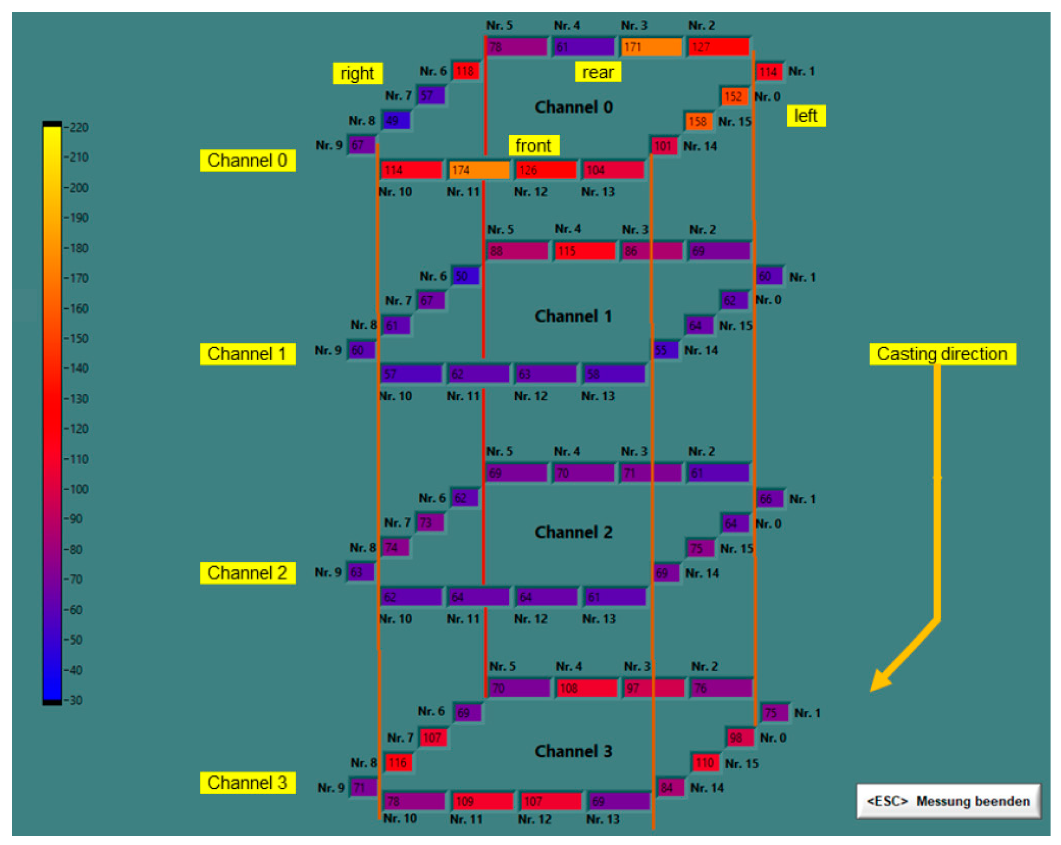
3.1.2. FOTS Measurements in Mould Walls at ESF

Figure 4 shows the layout of 64 optical temperature sensors arranged in four fibres within the mould wall, each with 16 sensors running around the mould perimeter at different distances of 0.1, 0.3, 0.5 and 0.65 m below the meniscus. The measurement technique uses the effect of temperature-dependent Bragg diffraction in the gratings imprinted on the fibres. In order to calculate the temperatures in the walls of the mould and compare them with the FOTS measurements, it would be necessary to model the heat transfer from the strand surface to the mould wall positions in detail as well as to model the further heat transfer from the mould wall to the cooling water box of the mould. This would involve further model parameters which cannot be tuned independently from the parameters ac, α of Equation (1) describing the heat flow density across the strand surfaces in the mould. Thus, only qualitative validations regarding the assumptions and calculations of the DynSolidCC model in the mould have been carried out. Thereby, the following conclusions could be drawn:
  • The symmetry assumption regarding heat flows across top/bottom and left/right strand surfaces and related measured FOTS temperatures fits better for the lower part of the mould (i.e., fibres 2 and 3) compared to the upper part (i.e., fibres 0 and 1). Moreover, the associated sensors near the middle of the walls show better congruence than those near corners.
  • After a significant decrease in measured mould wall temperatures from fibre 0 to fibre 1 to a level, which is more or less also measured at fibre 2, it increases again at fibre 3. At fibres 0 and 1, the top wall sensors have measured higher averaged temperatures than the left wall sensors. At fibre 2, all sensor measurements are quite close together, with mid-wall sensor results slightly higher than corner sensor results. At fibre 3, a symmetric temperature distribution can be observed with mid-wall values on an equal level significantly higher than the corner values, also on an equal level. This can be expected from the geometry with higher cooling effect from two faces near the edges and is related to the higher strand surface temperatures calculated at the middle of the strand compared to the temperatures at strand corners.
  • Thus, the heat transfer from the strand to the mould walls is homogenised in the range between fibre 1 and fibre 3, and for the lower part of the mould, the boundary conditions can be considered to be symmetric with respect to top/down and left/right strand surfaces.
  • Because the strand surface temperatures decrease with increasing distance from the meniscus, the observed increase in the mould wall temperatures at fibre 3 indicates an increase in the heat flow density by a better heat transfer at this mould length, e.g., due to better contact between strand surfaces and mould walls. This has been taken into account in the model parametrisation by choosing a more or less constant heat flow density at the strand surfaces along the mould length instead of a decreasing behaviour, which usually is suggested in the literature (see Equation (1)). However, simulations revealed no significant influence of the parameter α in Equation (1) on the strand temperatures and shell thicknesses at the mould exit if the total heat extraction across the mould is kept constant.
  • The comparison of temporal evolutions of measured mould wall temperatures and associated calculated strand surface temperatures shows a correlation where a decrease/increase in wall temperatures is related to an increase/decrease in strand surface temperatures with a delay of about 45 s. The FOTS along the mould measure decreasing/increasing heat flows between strand and mould, which lead to increasing/decreasing surface temperatures.
  • All in all, it seems justified to use the assumption of symmetric boundary conditions in the mould with a more or less constant heat flow density across the different strand surfaces. In the upper part of the mould, the non-homogenous steel flow conditions after inflow of the steel via the submerged entry nozzle (SEN) as well as the thinner strand shells and higher influences of mould-level fluctuations and non-uniform distributions of lubrication oil or powder lead to deviations from the symmetric boundary conditions which are reflected in the FOTS measurements at fibres 0 and 1. At fibre 2, there are already more homogenous heat transfer conditions which evolve towards fibre 3 to the expected case of more or less symmetric boundary conditions.

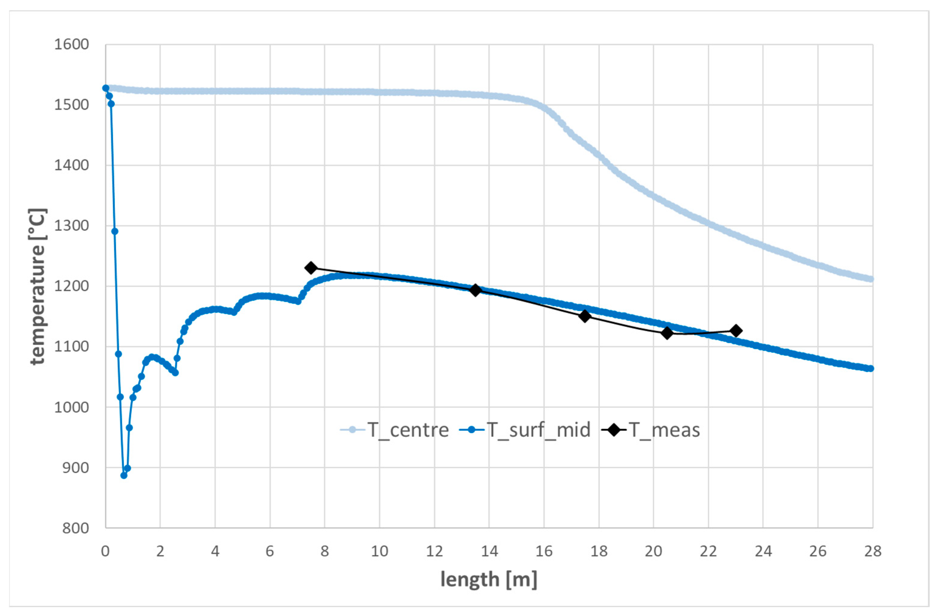
3.1.3. Infrared Camera Measurements of Strand Surface Temperatures at ESF

Feralpi used a handheld infrared camera available for one measurement campaign at ESF billet caster to determine the mid-surface temperatures on the left strand side (in casting direction) at five points:
  • On curved area;
  • After straightening;
  • Before descaling;
  • After descaling;
  • Before cutting torch.
The stationary casting conditions during these measurements have been logged by the online application of the DynSolidCC model. Based on the logged model input data, the casting process was simulated with variations in parameters ai, ar and br of Equations (3) and (4) describing the heat transfer coefficients in the secondary spray water and subsequent radiation zones, respectively. Thereby, an optimised parameter setting with a minimum mean square deviation between measured and simulated surface temperatures could be found. Figure 5 shows the related simulated stationary temperature profile for the given casting conditions and compares the simulated surface temperatures with the measured ones. For the latter, an emissivity of the strand surface of 0.8 has been assumed. The tuning of the mentioned boundary condition parameters resulted in a good agreement between measurement and simulation results.
In the next step, the simulated crater end position was compared to measurements of the vibrational spectrum of the strand, which is described in the following subsections.

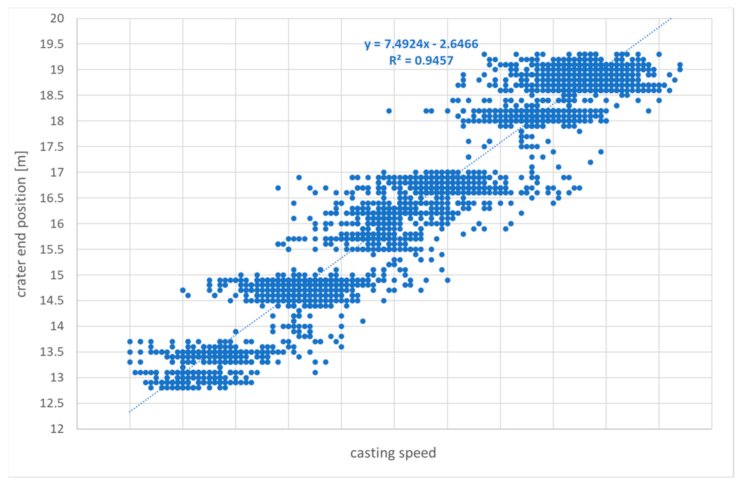
3.2. Vibrometer Measurements of Crater End Position at ESF

From the physics of vibrations of a solid with some liquid core, it is expected that the spectrum depends on the fraction of this liquid core, which allows identifying the crater end position in a strand of a continuous casting machine. Two measurement campaigns were conducted using a laser Doppler interferometer at the ESF billet caster with vibration excitations from the casting process itself:
  • First campaign with varying measurement positions and fixed casting conditions.
  • Second campaign with a fixed measurement position and varying casting conditions, i.e., increasing casting speed.
The acquired measurement data were pre-processed by Fast Fourier Transformation (FFT) and normalisation techniques and then analysed by means of Artificial Intelligence (AI) methods.

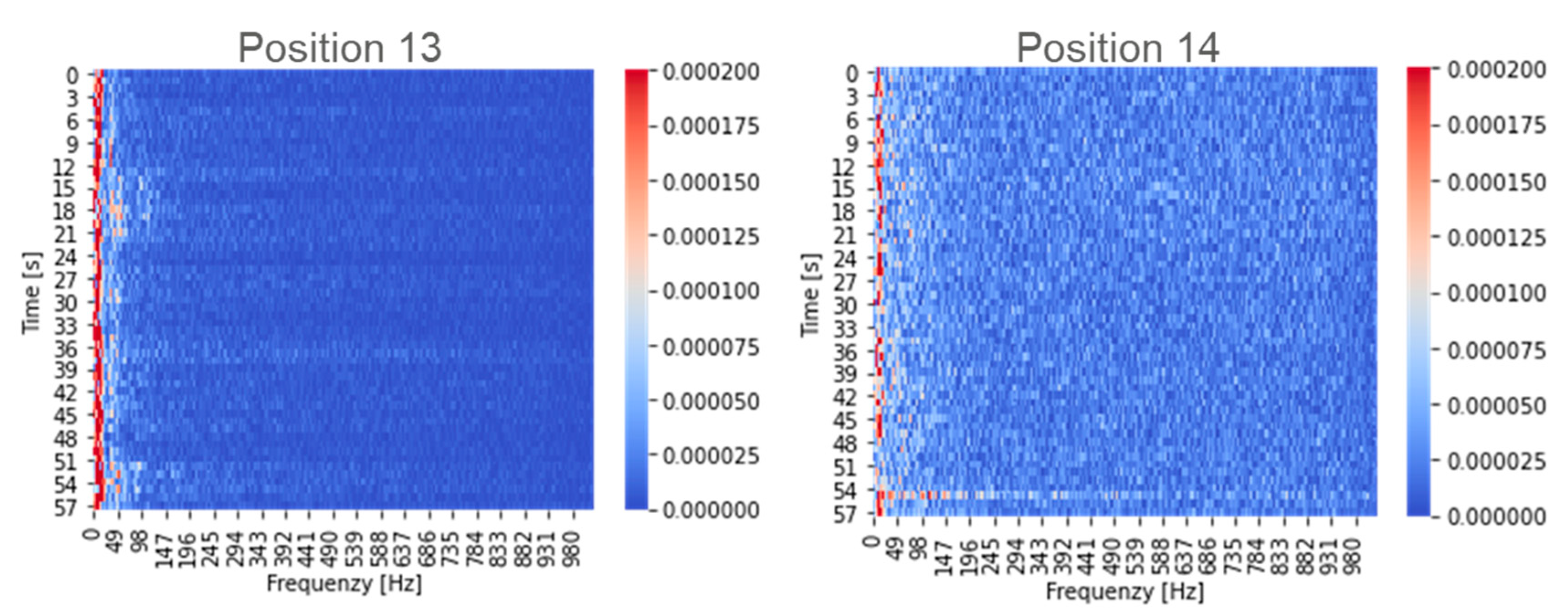
3.2.1. Vibrometer Measurement Campaign with Varying Strand Positions

Figure 1 shows the laser vibrometer mounted on a rail to measure the strand vibrations along different positions of the ESF billet caster:
  • 20 measurement points on strand from torch cutter over a length of 5 m;
  • 60 s measurement time for each measurement position;
  • 900 s measurement time at nearest and most distant position to the torch cutter;
  • 2 measurement sequences with two different casting speeds.
The pre-processing was performed by FFT of the raw vibrometer signal over measurement intervals of 1 s. Due to the mainly stationary casting conditions during the measurements, intervals of 1 to 60 s with frequency resolutions of 1 Hz to 1/60 Hz, respectively, are reasonable. This pre-processing step revealed significant differences in the transformed signal. However, these seemed to arise mainly from different characteristics of the positions themselves, e.g., due to the water jet of the descaling system evaporating on the strand surface (see Figure 6).
In order to verify this observation, the data were analysed with supervised machine learning methods, i.e., neural networks. For this purpose, the data were scaled based on the mean values and standard deviations of each frequency. The neural network’s hyperparameters were optimised using a tree-structured Parzen estimator, which is a single-objective Bayesian optimisation algorithm. The resulting structure of the chosen neural network is given by
  • Two hidden layers with 64 and 128 neurons;
  • Rectifier activation function;
  • Max. number of iterations = 500.
Applying the neural network to predict the measurement position using the transformed signal of a 1 s measurement interval yielded a 56% accuracy on the training and a 35% accuracy on the test data set. Considering that the confusion mainly happens between neighbouring positions (see Figure 7), it can be concluded that every measurement position along the steel strand has a characteristic vibration footprint that could overlay the influence of the strand solidification grade and make the detection of the crater end position difficult. This conclusion is also supported by the observation of the most significant transition of the vibration spectrum for the measurement sequences with both casting speeds between positions 13 and 14, which are before and behind the descaler, respectively. Therefore, a second vibrometer measurement campaign was performed with a fixed measurement position and varied casting conditions to avoid those positional effects.

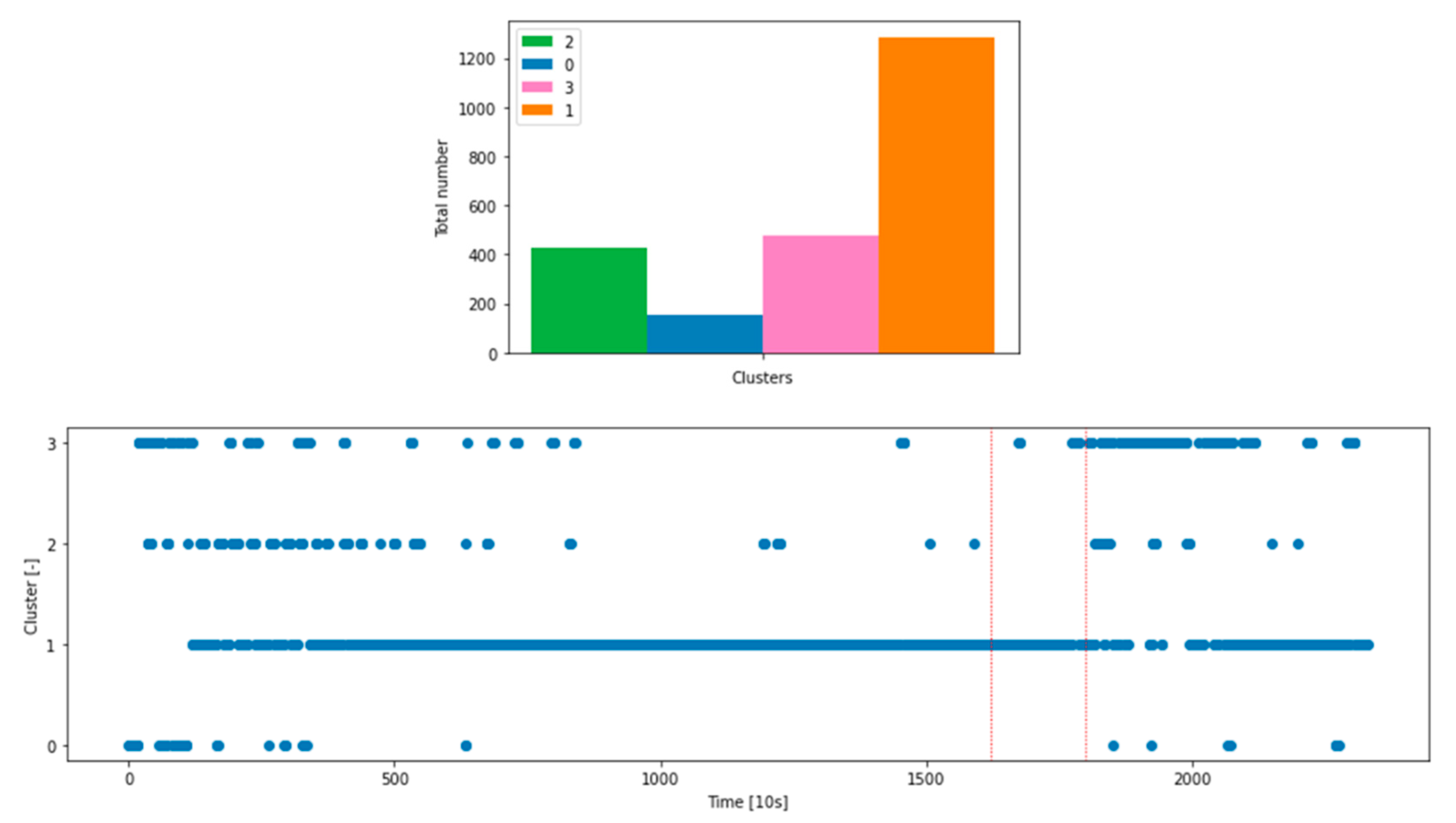
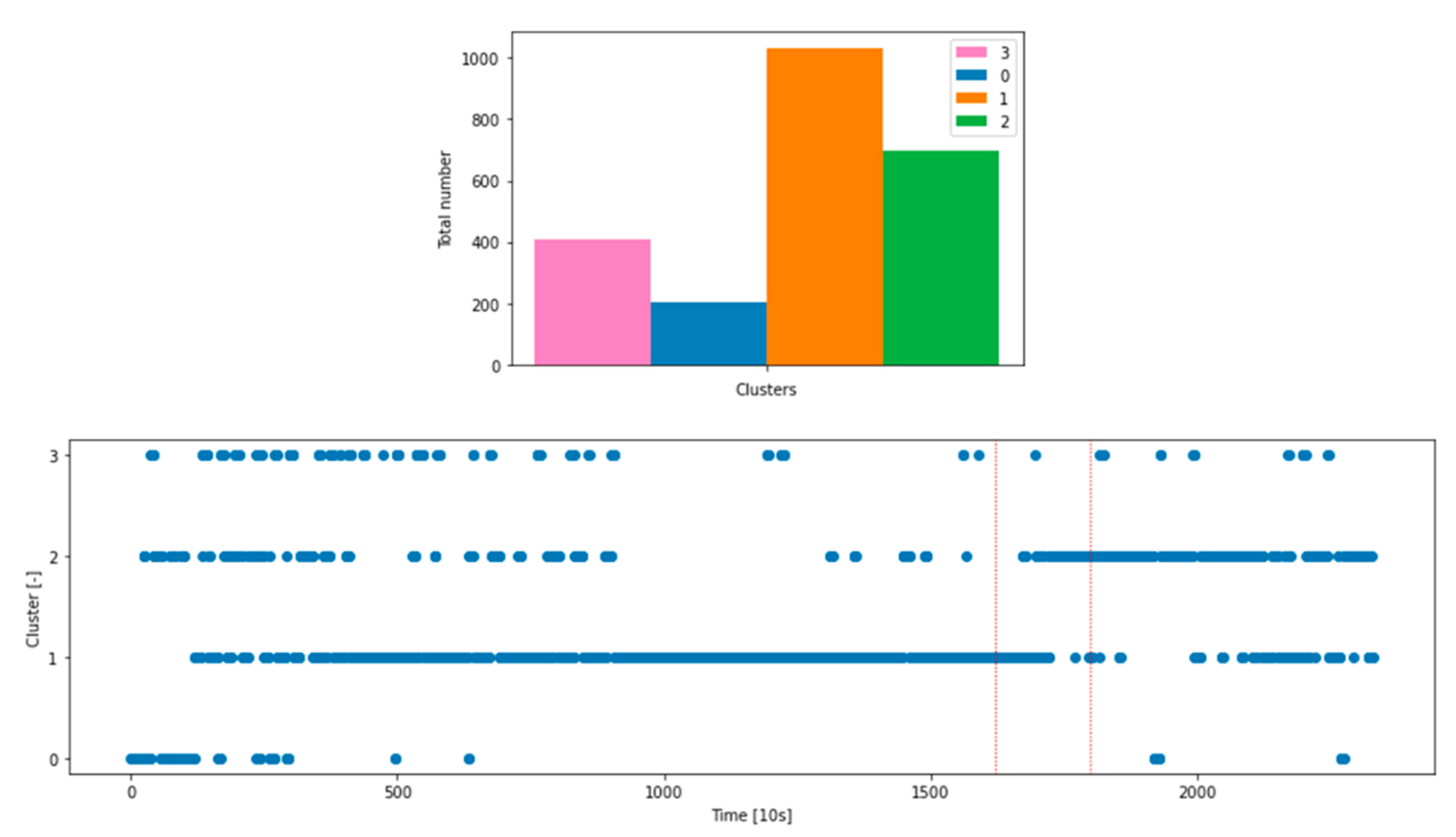
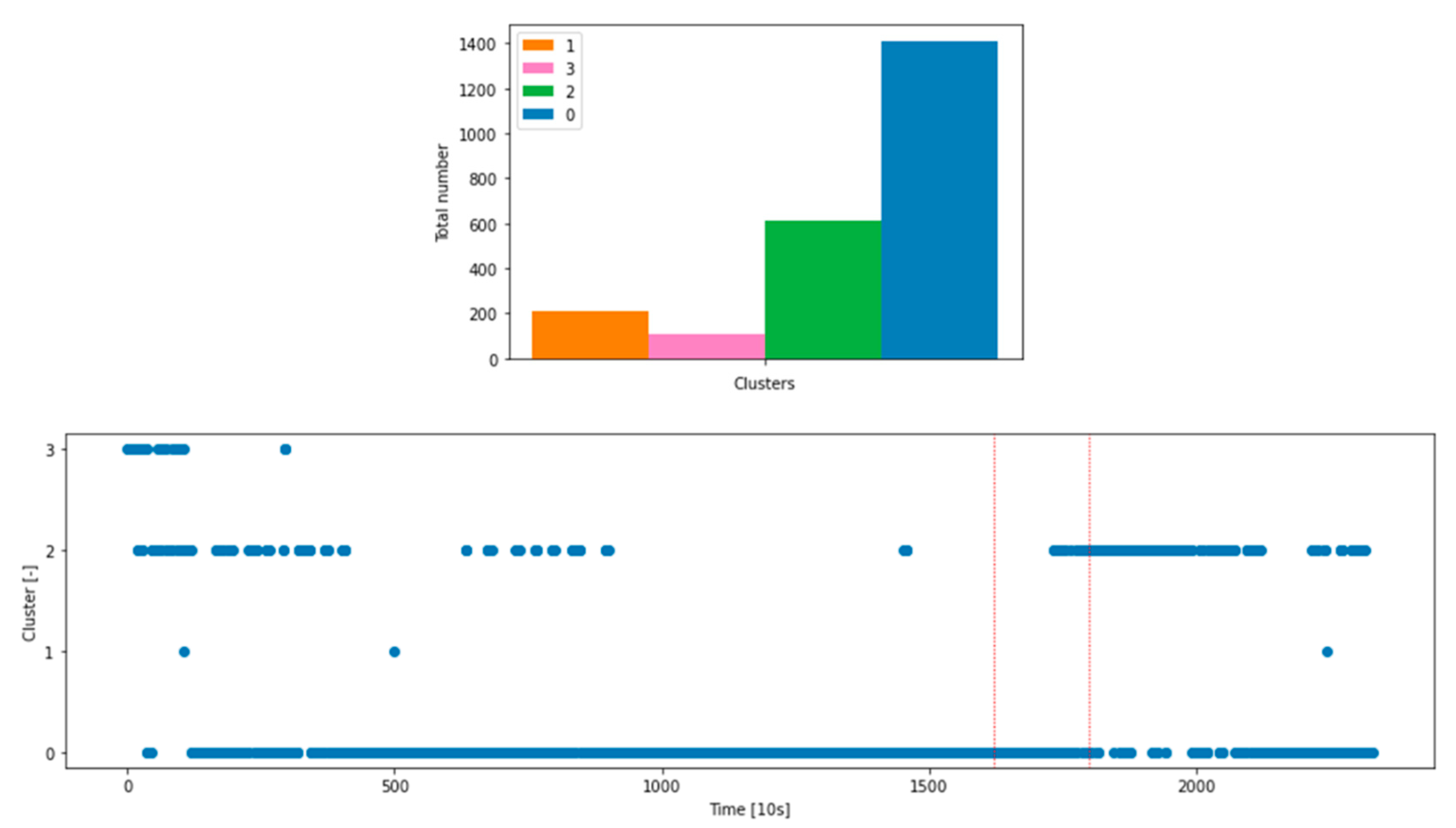
3.2.2. Vibrometer Measurement Campaign with Varying Casting Speeds

By increasing the casting speed, the crater end position is expected to move through a fixed measurement position of the laser vibrometer mounted at a distance of about 16–19 m below the meniscus. For that purpose, the measurement conditions were chosen as follows:
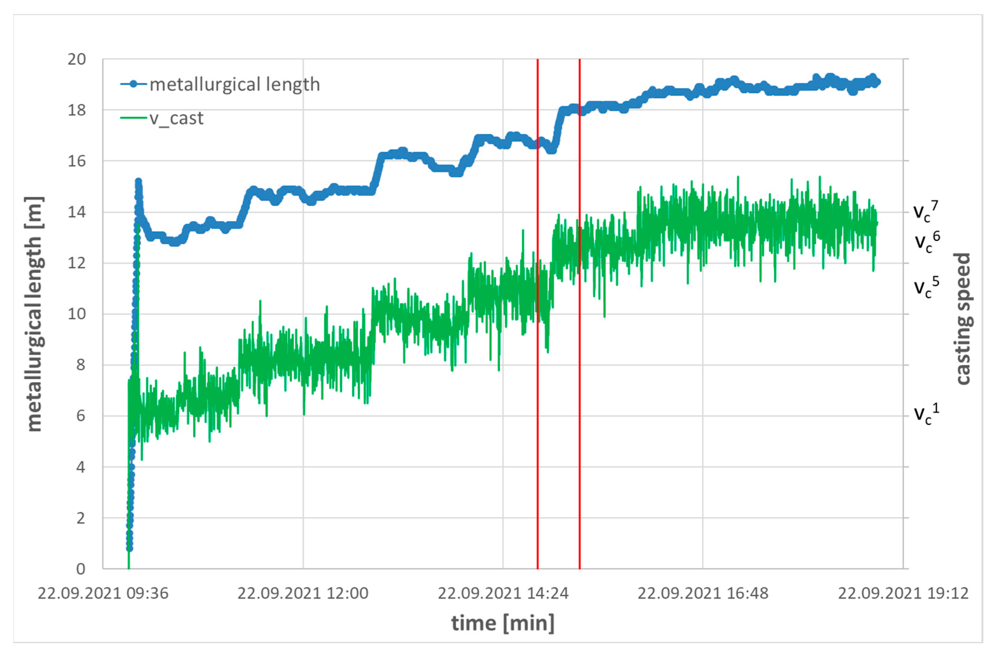
  • Continuous measurement at 17.5 m below the meniscus with seven casting speeds increasing from vc1 to vc7.
  • Two 30 min measurements after changes in casting speed to measure during transitional and stationary conditions.
The pre-processing steps were similar to the first measurement campaign, but additionally, FFTs with 10, 30 and 60 s measurement intervals were analysed. In order to detect the passing of the crater end at the measurement position, unsupervised learning methods in terms of clustering approaches were used for this campaign, which are supposed to reveal significant differences in the frequency spectrum of fully solidified strands and those with a liquid core.
The number of optimal clusters was derived using the elbow method with the classical K-means algorithm, which led to a total of four clusters. Three clustering algorithms were applied overall:
  • K-means;
  • Gaussian mixture model;
  • Hierarchical clustering with Ward linkage.
The results are depicted in Figure 8, Figure 9 and Figure 10 for FFTs with a 10 s measurement interval, as this configuration revealed the best results. The upper figures show the number of measurement points (i.e., 10 s intervals) that each identified cluster contains, and the bottom figures show the temporal development of the cluster prediction during the measurement campaign. The casting velocity was increased incrementally towards the end of the campaign. Thus, it was expected that the crater end moves during the campaign from a position before the vibrometer, where the strand at the vibrometer is completely solidified, to a position behind the vibrometer, where the strand at measurement position has a liquid core. Note that the depicted clusters in the bottom figures are a moving average over the last 10 forecasts to smoothen the data and highlight transitions more clearly.
(1)
K-means algorithm
The K-means algorithm clusters data by trying to separate samples in different groups of equal variance, minimising a criterion known as the inertia. This algorithm requires the number of clusters to be specified. It scales well to a large number of samples and has been used across a wide range of application areas in many different fields.
(2)
Gaussian mixture model
A Gaussian mixture model is a probabilistic model that assumes that all the data points are generated from a mixture of a finite number of Gaussian distributions with unknown parameters. One can think of mixture models as generalising K-means clustering to incorporate information about the covariance structure of the data as well as the centres of the latent Gaussians.
(3)
Hierarchical clustering
Hierarchical clustering is a general family of clustering algorithms that build nested clusters by merging or splitting them successively. This hierarchy of clusters is usually represented as a tree (or dendrogram). The root of the tree is the unique cluster that gathers all the samples, the leaves being the clusters with only one sample. Ward linkage minimises the sum of squared differences within all clusters. It is a variance-minimising approach and in this sense similar to the K-means objective function but tackled with an agglomerative hierarchical approach.
Figure 8, Figure 9 and Figure 10 show that all three approaches detect
  • Transient effects during the beginning of the measurement campaign with significant population of more than two clusters, which reflects the associated unsteady strand conditions of the start of casting phase;
  • A transition in population of the two most frequently predicted clusters after a measurement time between 16,200 and 18,000 s (4.5–5.0 h, indicated by red vertical lines), where the casting speed increased from vc5 to vc6.
The latter observation can be related to the passing of the crater end at the measurement position of the vibrometer. This is in accordance with the model simulation of the evolution of the metallurgical length (i.e., the crater end position) during the measurement campaign, as shown in Figure 11. This figure displays the casting speed increasing in several steps from vc1 to vc7 and the resulting movement of the crater end position from about 13 m to 19 m below the meniscus. After an increase in the casting speed from vc5 to vc6, the crater end moves from about 17 m to 18 m, i.e., it passes the position of the vibrometer at 17.5 m (cf., period between red vertical lines in Figure 11). Thus, with some caution and under certain reservation, the observed transition in the population of the vibrational clusters can be assessed as a footprint of the passed crater end position with a change from a fully solidified strand to a strand with some liquid core. The found parametrisation of the dynamic solidification model could be confirmed with respect to the calculated crater end position with an accuracy of about +/− 0.5 m. Note that this conclusion relies on only one measurement campaign. For broader validation, further similar investigations would be helpful, which unfortunately were not possible anymore within the ConSolCast project.

3.3. Dynamic Control of Crater End Position

3.3.1. Parameter Studies Regarding Influence of Different Casting Parameters on Strand Temperature and Solidification Front

The dynamic temperature and solidification model DynSolidCC developed by BFI was used within appropriate offline simulations for parameter studies regarding the influence of the following parameters on the resulting temperature profile and solidification front in the billet caster at ESF:
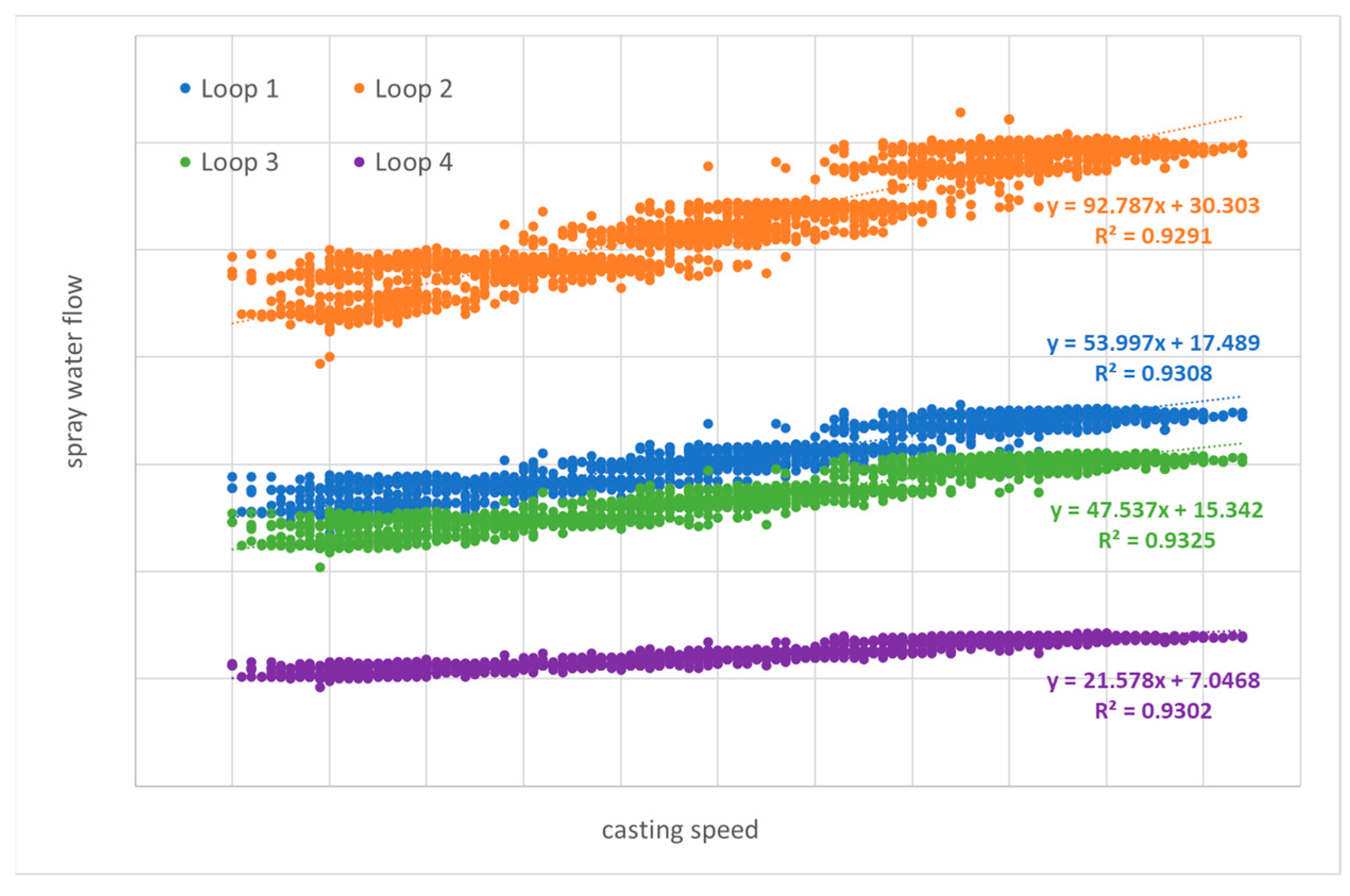
  • Spray water flows in secondary cooling zone;
  • Casting speed;
  • Initial superheat of steel.
These casting parameters have been varied from a defined reference case.
(1)
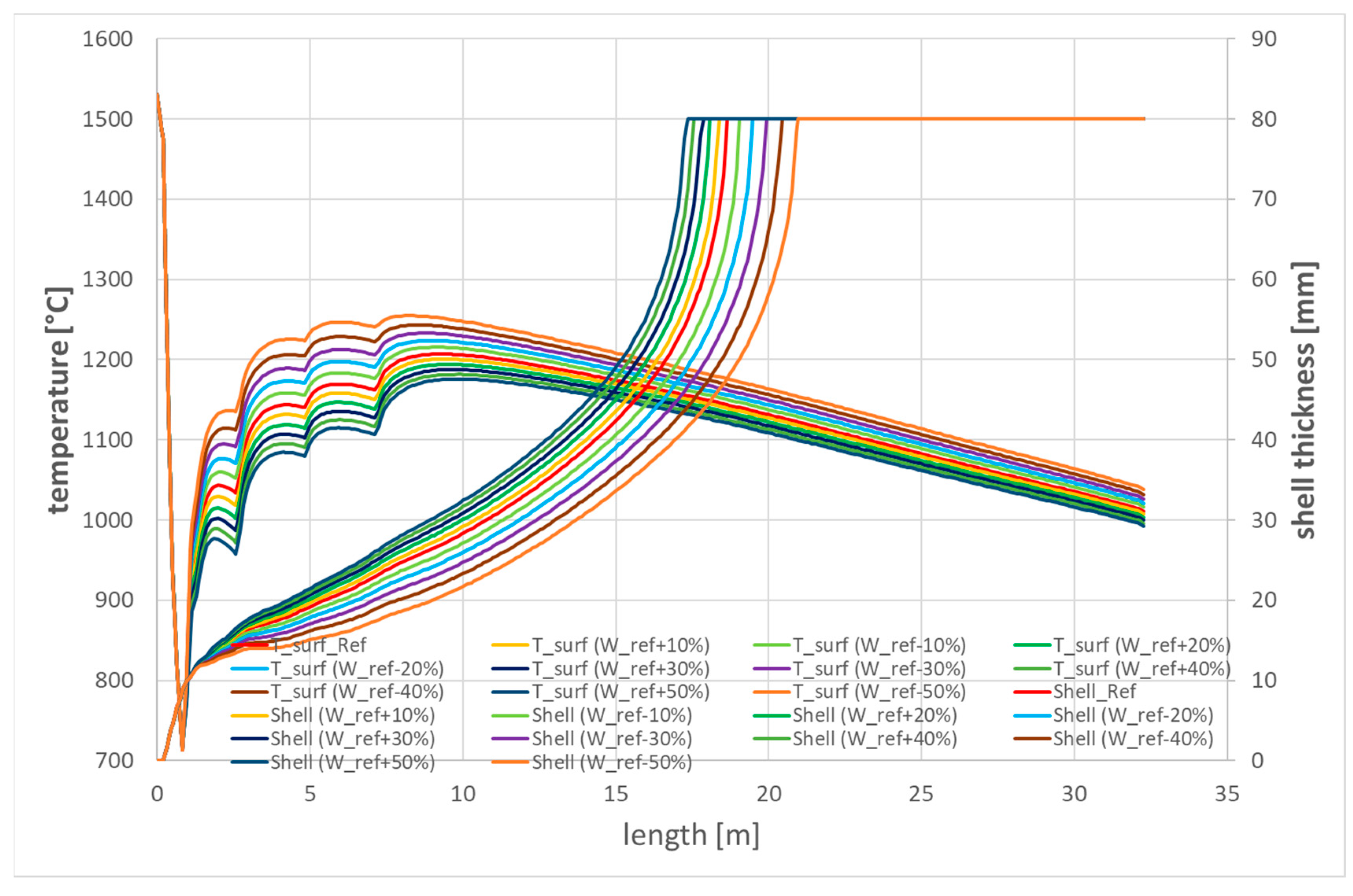
Variation of spray water flows in secondary cooling zone
In a first parameter study, the spray water flows for the four secondary cooling loops have been varied between values of 50% and 150% of the flow rates defined for the reference case. The other casting conditions were kept constant. Figure 12 shows the surface temperature and shell thickness for the middle of the strand top side resulting from the offline simulations with the DynSolidCC model for the different cases of applied spray water flows:
  • At the end of the last spray water cooling loop, the mid-surface temperatures decrease with the first 10% increase in spray water (from 50% to 60% of reference flow rates) by 19 K and with the last 10% increase (from 140% to 150% of reference flow rates) by 10 K.
  • The maximum difference in surface temperatures between the cases of 50% and 150% of reference spray water flow at the end of the last cooling loop is about 135 K;
  • It decreases to about 54 K at a length of 23 m, where the cutting torch is located.
  • The crater end position moves from 17.4 m for the case with the highest spray water cooling to 21.0 m for the case with the lowest cooling.
  • With the first 10% increase in spray water (from 50% to 60% of reference flow rates), the crater end position decreases by 0.58 m, and with the last 10% increase (from 140% to 150% of reference flow rates) by 0.26 m.
(2)
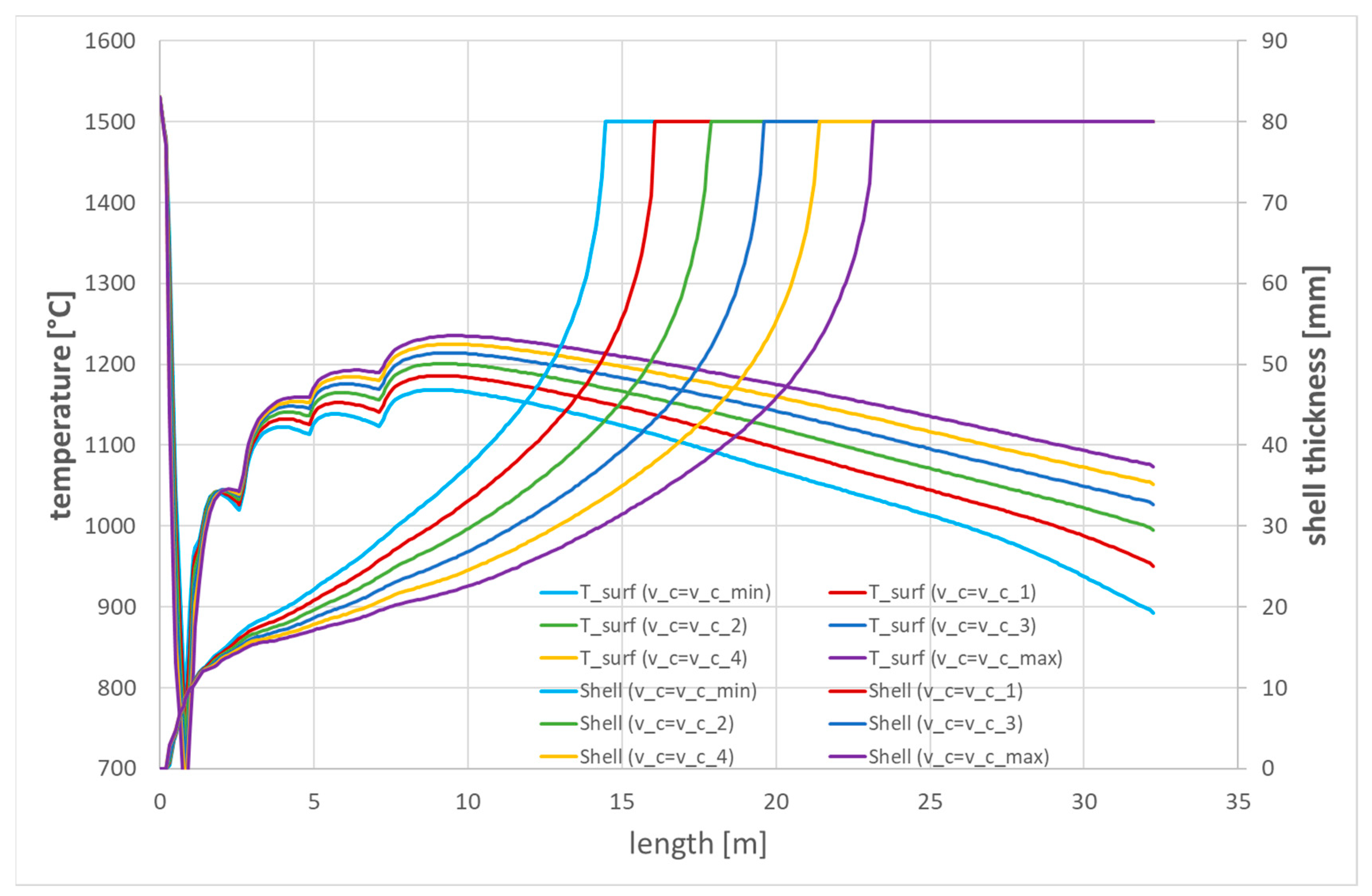
Variation of casting speed
In a second model simulation campaign, the influence of variations in the casting speed between vcmin and vcmax on the temperature field and solidification front of the strand was studied. In order to take into account the increased heat transfer in the mould with increasing casting speeds, the related heat flow densities across the strand boundary were scaled appropriately with the casting speed vc by a factor vc/vcref, where vcref is the reference casting speed. The other defined reference casting conditions were kept constant. Figure 13 shows the simulated surface temperature and shell thickness for the middle of the strand top side for the different cases of applied casting speed:
  • At the end of the last spray water cooling loop, the mid-surface temperatures increase with the first increase in casting speed Δvc by 18 K and with the last increase by 9 K.
  • The maximum difference in surface temperatures between the casting speed cases of vcmin and vcmax at the end of the last cooling loop is about 66 K;
  • It increases to about 113 K at a length of 23 m, where the cutting torch is located.
  • The crater end position moves from 14.5 m for the case with the lowest casting speed to 23.2 m for the case with the highest casting speed.
  • With the first increase in casting speed Δvc, the crater end position increases by 1.6 m, and with the last increase by 1.8 m.
Thus, the increase in the crater end position by 0.8–0.9 m per increase of 0.1 m/min in casting speed is more homogenous than observed with decreasing spray water flow rates. All in all, the found decreases in surface temperatures and crater end position with incrementally increasing spray water flows as well as decreasing casting speeds have been identified as an appropriate basis for a dynamic cooling strategy via the secondary cooling loops.
(3)
Variation of superheat of steel poured into the mould
Finally, in a third parameter study, the initial temperature of the steel poured into the mould was varied between T0min and T0max, which is between ΔTmin and ΔTmax above the liquidus temperature of the investigated steel grade. The other casting conditions were kept constant according to the defined reference case. Figure 14 shows the surface temperature and shell thickness for the middle of the strand top side resulting from the model simulations for the different initial steel temperatures.
  • At the end of the last spray water cooling loop, the mid-surface temperatures increase with each increase of 5 K regarding the initial steel temperature by about 3.4 K.
  • The maximum difference in surface temperatures between the cases with initial steel temperature of T0min and T0max at the end of the last cooling loop is about 17 K;
  • It decreases to about 13 K at a length of 23 m, where the cutting torch is located.
  • With each increase of 5 K regarding the initial steel temperature, the crater end position moves by about 0.2 m towards the cutting torch.
  • By increasing the initial steel temperature from T0min to T0max, the crater end position moves from 18.0 m to 19.0 m.
Thus, the initial superheat of the steel poured into the mould has only a minor influence on the temperature field and solidification behaviour in the strand, compared to the higher influence of the spray water flows in secondary cooling and the even stronger influence of the casting speed.

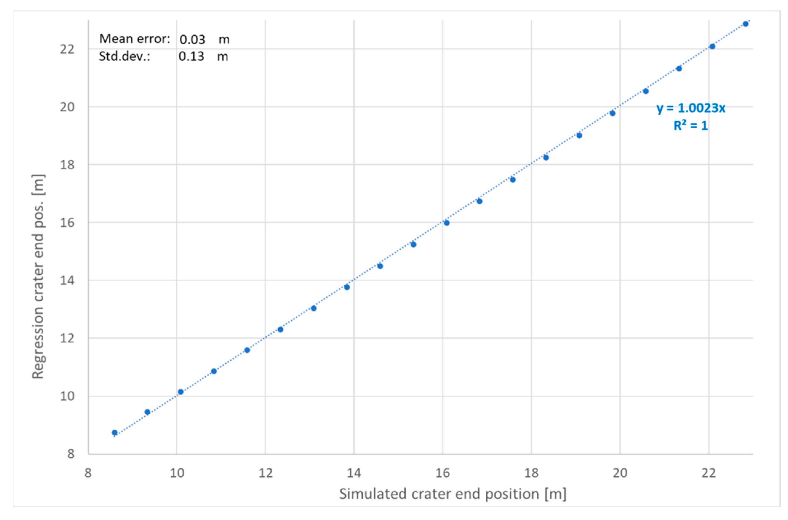
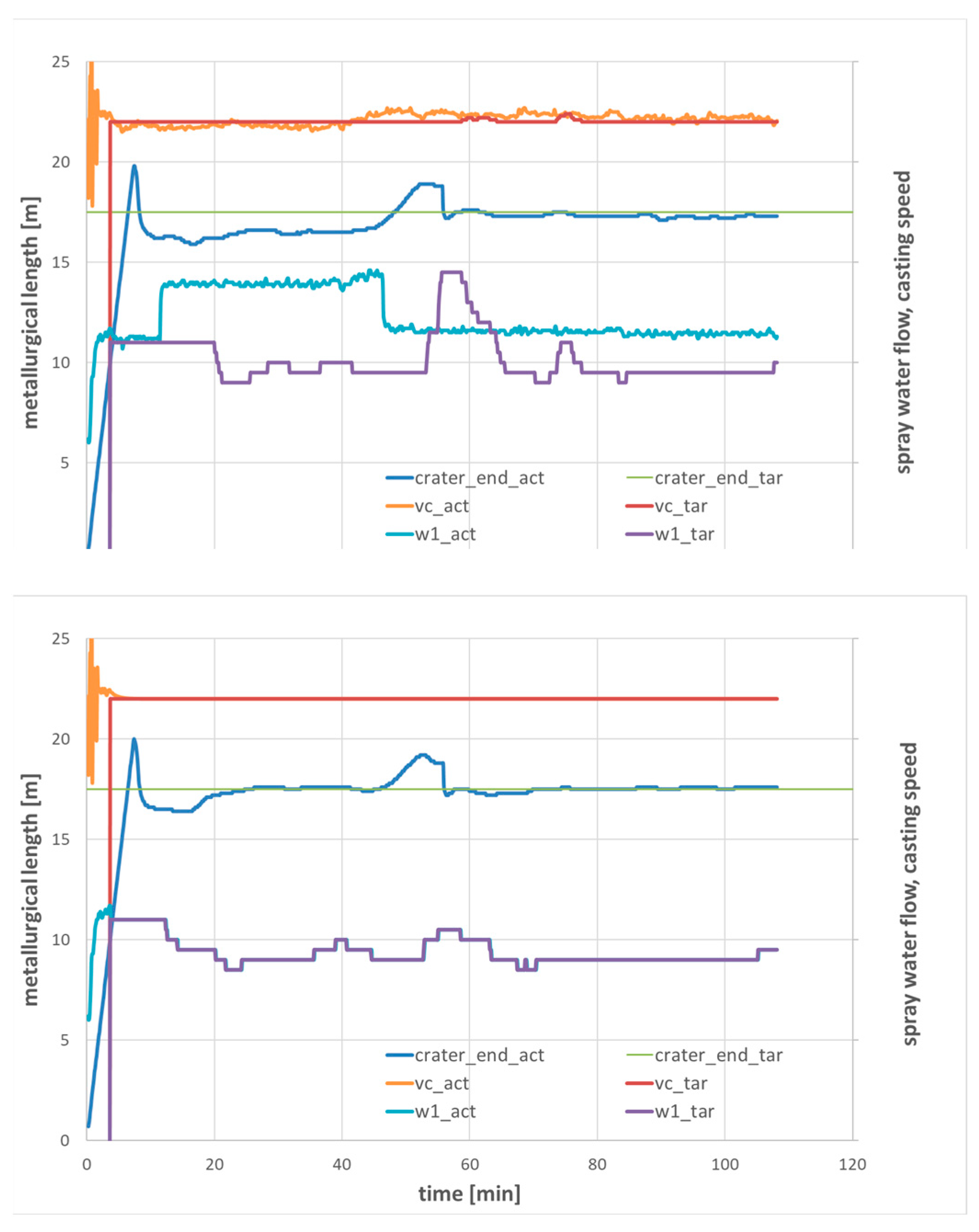
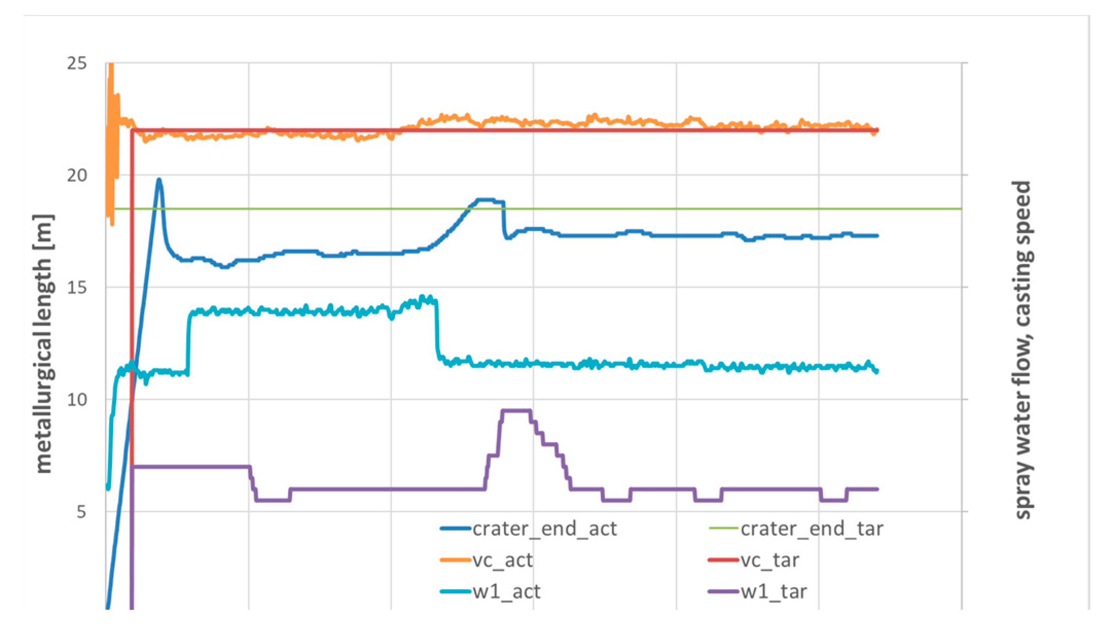
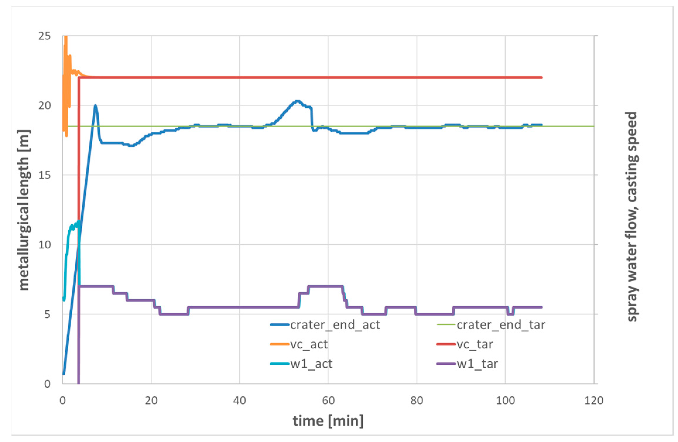
3.3.2. Dynamic Adaptation of Casting Speed and Spray Water Flow Rates

Two approaches of model-based dynamic control of casting conditions in order to adjust defined target quality parameters for the strands in the billet caster of ESF have been investigated.
In the first approach, based on heuristic rules in combination with methods for nested intervals (such as the “Pegasus” algorithm, an improved “Regula Falsi” method), the casting parameters (such as spray water flow rates and casting speed) are iteratively altered with subsequent model simulation of the resulting stationary three-dimensional temperature field and solidification state; the iteration is stopped, when within defined tolerances, the simulated strand quality parameters agree with the target values. However, this approach with up to 10 iterative simulations of stationary strand states requires too much calculation time (>1 s per iteration) for an online application with cyclic recalculation of the current strand state and adapted control casting parameters each 5–10 s (on the available hardware at ESF).
Thus, a second approach has been chosen, based on evaluations of the parameter studies for the ESF billet caster, which have been carried out with appropriate offline model simulations (cf., Section 3.3.1.). The ESF billet caster has only limited space behind the cutting torch. Thus, the adjustment of the crater end position to a defined target value has been identified as a useful dynamic control application.
The variation of the crater end position pos_CE with respect to the reference value pos_CE_ref simulated for the defined reference casting conditions (d_pos_CE = pos_CE − pos_CE_ref) under variation of (a) the casting speed (by d_v_c = v_c − v_c_ref) and (b) the spray water flow (by d_SPW = 100 × (SPW_i − SPW_i_ref)/SPW_i_ref for each loop i = 1…4) is shown in Figure 15. The dependency of the crater end position from the casting speed can be expressed by a linear equation:
d_pos_CE = a × d_v_c
whereas the dependency of the crater end position from the spray water flow is given by a quadratic equation:
d_pos_CE = c × d_SPW2 − b × d_SPW
Equations (5) and (6) are used to calculate the crater end position for casting speeds and spray water flows within a certain range of deviations d_v_c and d_SPW from the defined reference values by the regression formula:
pos_CE = pos_CE_ref + c × d_SPW2 – b × d_SPW + a × d_v_c
The reference value for the crater end position at reference casting speed and spray water flows may depend on the initial temperature and composition of the steel powered into the mould. The mould cooling water flow is more or less constant at ESF billet caster and the temperature increase in the mould cooling water scales (more or less linear) with the casting speed, which has been taken into account within the parameter studies leading to Equation (5). With variations of the spray water flow between d_SPW_min = −50% and d_SPW_max = +50% of the reference flow rates, an adjustment of the crater end position between d_pos_CE_min = −1.3 m and d_pos_CE_max = +2.3 m is achievable (cf., Figure 15b). Beyond this range, the crater end position has to be controlled via the casting speed.
Statistical evaluation of a real sequence casted at ESF with a certain range of different casting speeds revealed linear dependencies of the spray water flow rates and the resulting simulated crater end position from the chosen casting speed (cf., Figure 16 and Figure 17). Figure 18 shows good agreement of the crater end positions calculated from the regression Formula (7) for this casting sequence with the related values derived from the online model simulation extrapolated to a range of casting speeds between 1.5 and 3.4 m/min.
This agreement of the derived crater end positions confirms the possibility to use the simple regression Formula (7) instead of the more complex 3D simulation model to determine appropriate spray water flows and casting speeds for adjustments of given target crater end positions. Such an approach is also suitable for online applications with cyclic recalculations each 5–10 s. The implemented dynamic control procedure to be carried out within each cyclic calculation of the strand state is summarised in Appendix A.
The real ESF casting sequence from Figure 16, Figure 17 and Figure 18 has been simulated and investigated with respect to the calculated set-points for different targets of the crater end position. For each of the defined targets, the simulation has been performed in a first scenario without and in a second scenario with using the calculated set-points for casting speed and spray water flows in the further casting process. Figure 19, Figure 20, Figure 21, Figure 22 and Figure 23 show the resulting evolutions of actual and target casting speed, spray water flow and crater end position for defined target crater ends of 15 m, 16.5 m, 17.5 m, 18.5 m and 20 m, respectively. The spray water flows are displayed for the first cooling loop, the flows of the other loops have an analogue evolution on the scale of the respective reference flow rate. After an initial start of casting phase of about 20 min, the strand achieves a first stationary state. After about 45 min, there is a change to another steel grade with some transient behaviour, which about 10 min later results in a new stationary phase with a new crater end position in the actual casting process and the same target position in the dynamically controlled process.
The adjustment of a target crater end position of 15 m leads to maximum set-points for the spray water flows (50% higher than reference flow rates) and casting speed set-points below the values of the actual process (cf., Figure 19). For the adjustment of a target crater end position of 16.5 m, the control procedure suggests similar set-points for spray water flows and casting speed as applied in the actual process for the first steel grade. After the grade change, the actual process operates with slightly increased casting speed and decreased spray water flows, whereas the controlled process suggests the same set-points for the second stationary phase as for the first grade to keep the casting position at the target value. Here, the reference casting speed can be chosen for the whole process (cf., Figure 20). With target crater end positions of 17.5 m and 18.5 m, the set-points for spray water flows are decreased further on below the flow rates applied in the actual process (cf., Figure 21 and Figure 22).
Finally, the adjustment of a target crater end position of 20 m results in minimum set-points for the spray water flows (50% lower than reference flow rates) and casting speed set-points above the values of the actual process (cf., Figure 23). All in all, the case study based on the real casting sequence of ESF confirmed the capability of the developed dynamic cooling strategy to control the crater end position within a suitable operational range of the ESF billet caster.

3.4. Operator Information and Advisory System

The API of the model kernel developed by BFI is used by a model shell developed by ESF for communication between the ESF automation system and the DynSolidCC model. There is a permanent exchange between model, database and Programmable Logic Control (PLC). An extended visualisation and user interface has been developed and installed at ESF billet caster with focus on simplification and user-friendliness for the operator. With this user interface, the operator can select specific data to be displayed or evaluated. Figure 3 shows a screenshot of the extended HMI integrated within the production mask.
The user interface shows for a selected distance from the meniscus in the mould a coloured cross-section of the strand produced by the currently casted batch (“Produktnummer”, cf., Figure 3, left side). It distinguishes within a 17 × 17 field different temperature ranges depending on the temperatures calculated by the model. Inside the cross-section, the shell thickness is visualised by a black line. It is also displayed numerically (“Schalendicke”) in millimetres together with the crater end position (“Sumpfspitze”) in metres for the target and the calculated actual state. Point 8 of the example in Figure 3 is at 0.86 m below the meniscus, i.e., at the exit point of the mould. This point was deliberately chosen because there the shell must be stable enough to withstand the ferrostatic pressure. A sufficiently thick strand shell prevents breakouts. The user has the option to view and evaluate the temperature and solidification state at other positions by using a slider (cf., Figure 3, centre left). If the slider is moved, the model results for the selected position are transferred to the HMI. Additionally, a top view of the caster and the strand is displayed. Here, the casting parameters along the strand related to the primary cooling in the mould and the secondary cooling in the spray water zones 1–4 are shown to the user (cf., Figure 3, centre right).
The huge amount of data calculated by the model and the high number of measured parameters cannot be processed in their entirety by the operator. Therefore, a traffic light system has been integrated into the HMI which compares defined collected and calculated data of a strand with specified limit values (cf., Figure 3, right side). If a parameter deviates from the specification, the traffic light switches its colour from green (regular range) to yellow (critical range) or red (dangerous range). Thereby, the operator can localise the cause of irregular casting conditions and intervene, if necessary. Such an intervention may result in a shutdown of the irregularly running strand in order to prevent a possible breakout event. The most important and influencing parameters analysed and visualised by the traffic light system comprise:
  • Temperature in tundish (“Verteilertemperatur”);
  • Temperature of mould water inlet (“Kokillenwasser-EinlassTemp.”);
  • Temperature difference between mould water outlet and inlet (“Kokillenwasser-Temp.-Diff.”);
  • Flow rate of mould water (“Kokillenwasserdurchfluss”);
  • Pressure of spray water zones 1–4 (“Spritzwasserdruck”);
  • Crater end position calculated by DynSolidCC model (“Position Sumpfspitze”);
  • Shell thickness at mould exit calculated by DynSolidCC model (“Schalendicke …”).
Finally, the output of recommendations calculated by the dynamic cooling control function based on the DynSolidCC model are also visualised in the HMI (cf., Figure 3, right side, “Modellempfehlung”). These recommendations help the operator to properly adjust the spray water flow rates and casting speed (by using another submerged entry nozzle) in order to achieve a given target value for the crater end position. Thus, they are an important contribution to prevent potential breakouts due to dangerous ranges of the actual crater end position.

4. Discussion

The ConSolCast project dealt in detail with the topic of strand breakouts and surface defects and developed measurement techniques and model-based tools to minimise such casting anomalies. At ESF, this led to the installation of a new operator information and advisory system with an appropriately extended HMI. This approach for online monitoring and control of the billet casting process was focused on the real-time visualisation of
  • Measured casting parameters;
  • Simulated 3D temperature field, shell thickness along the strand length and actual crater end position;
  • Traffic lights regarding possibly critical or dangerous values for selected casting parameters, shell thickness and crater end position;
  • Suggested casting speed and spray water flow rates to adjust a given target crater end position.
A disadvantage of the implemented traffic light procedure is that a strand may be closed, where a breakout would not occur in each case. However, the advantages of this procedure outweigh the disadvantages, because a real breakout could damage plant components or cause longer downtimes. Thus, avoidance of such possible breakouts or preventing casting failures improves the casting process in terms of
  • Higher machine availability, i.e., productivity;
  • Higher safety;
  • Lower maintenance costs.
With the introduction of the traffic light system in combination with the DynSolidCC model-based monitoring and control functions, the breakout rate could be decreased from about 2–3% (which is typical for the industry) to values of about 1–1.5%.
The recording of the temperatures within the mould could successfully provide measurement data, which were used as a basis for the validation and adaptation of the DynSolidCC mould boundary condition submodel. Additional measurements of strand surface temperatures with an infrared camera allowed adjusting the boundary condition model parameters for the spray water and radiation cooling zones of the caster. Moreover, the measurement campaigns with the laser vibrometer revealed that the simulated evolution of the crater end position fits well with the measured footprint of a completely solidified strand in the recorded vibrational spectra. This finding shall be investigated in the future also for other casting formats and qualities in order to establish a new measurement technique for assessment of the solidification state in a strand during continuous casting processes.

Author Contributions

Conceptualisation, M.S., M.G. and P.F.; Data curation, R.S. and J.B.; Funding acquisition, M.S., M.G. and P.F.; Methodology, M.S., M.K. and W.K.; Project administration, M.S., M.G. and P.F.; Resources, M.S., M.G. and P.F.; Software, M.S., W.K. and J.B.; Supervision, M.S., M.G. and P.F.; Validation, M.G. and R.S.; Writing—original draft, M.S.; Writing—review and editing, M.K., W.K., M.G., R.S., J.B. and P.F. All authors have read and agreed to the published version of the manuscript.

Funding

This research was funded by the Research Fund for Coal and Steel under grant agreement no. 799295.

Institutional Review Board Statement

Not applicable.

Informed Consent Statement

Not applicable.

Data Availability Statement

Not applicable.

Conflicts of Interest

The authors declare no conflict of interest. The funders had no role in the design of the study; in the collection, analyses, or interpretation of data; in the writing of the manuscript; or in the decision to publish the results.

Appendix A

The implemented procedure for dynamic control of the crater end position can be summarised by the following steps to be carried out within each cyclic calculation of the strand state (the names of the involved variables and parameters are explained in Section 3.3.2):
  • After achievement of defined minimum casting length:
    Initialise target casting parameters based on regression Formula (7) for given target crater end position with default reference value.
  • Check stationary casting conditions, i.e., variations of casting speed, spray water flows and simulated crater end position are within defined tolerances.
  • Instationary state → keep target casting parameters from previous cyclic calculation.
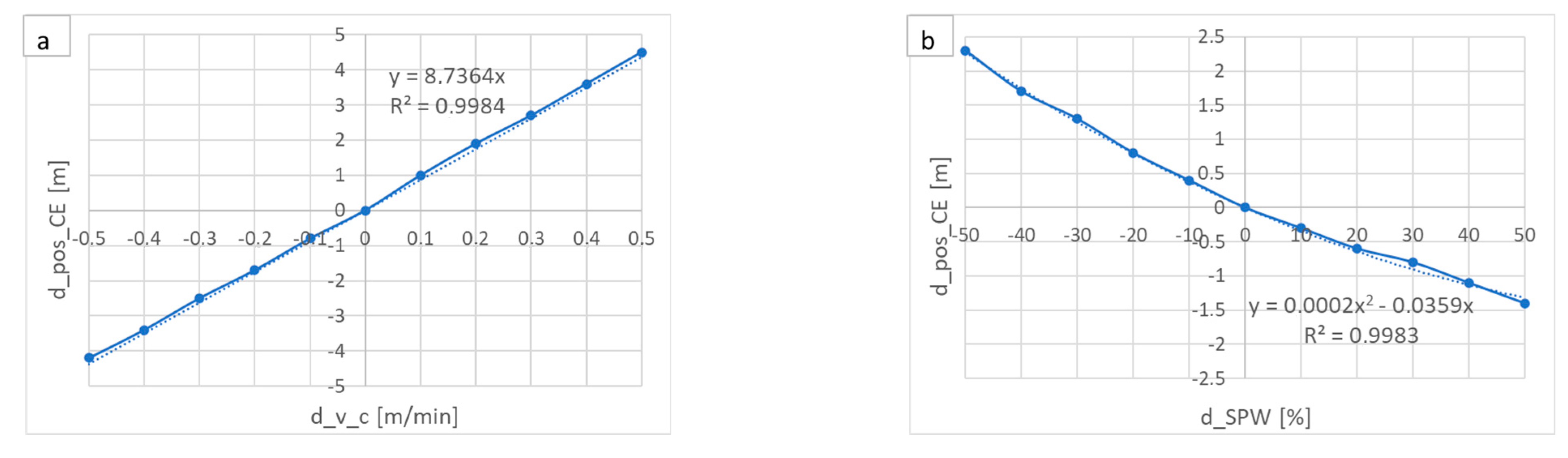
  • Check deviation of simulated crater end position from target value:
    ∆pos_CE = pos_CE – pos_CE_tar
  • Stationary state and |∆pos_CE| within defined tolerance:
    → keep actual casting parameters:
    SPW_i_tar   = SPW_i
    v_c_tar   = v_c
  • Stationary state and |∆pos_CE| outside defined tolerance:
    → calculate target casting parameters from regression Formula (7):
    o
    Determine reference crater end position:
    pos_CE_ref = pos_CE – (c * d_SPW2 – b * d_SPW + a * d_v_c)
    o
    Check d_pos_CE_tar = pos_CE_tar – pos_CE_ref:
    i.
    d_pos_CE_tar ≥ d_pos_CE_min and d_pos_CE_tar ≤ d_pos_CE_max:
    d_SPW_tar   = b/(2c) – (b2/(4c2) + d_pos_CE_tar/c)1/2
    d_v_c_tar     = 0
    ii.
    d_pos_CE_tar < d_pos_CE_min:
    d_SPW_tar   = d_SPW_max
    d_v_c_tar     = (d_pos_CE_tar - d_pos_CE_min)/a
    iii.
    d_pos_CE_tar > d_pos_CE_max:
    d_SPW_tar   = d_SPW_min
    d_v_c_tar     = (d_pos_CE_tar - d_pos_CE_max)/a
    o
    Check correction of target casting parameters based on comparison with actual ones: ∆SPW = 100 * (SPW – SPW_tar)/SPW_ref, ∆v_c = v_c – v_c_tar
    with thresholds εSPW, εv_c > 0 to be exceeded in case of significant difference |∆pos_CE| > εCE:
    i.
    ∆pos_CE > εCE and ∆SPW > - εSPW and ∆v_c < εv_c:
    d_SPW_tar’ = d_SPW_tar + εSPW,   d_v_c_tar’ = d_v_c_tar
    if d_SPW_tar’ > d_SPW_max:
    d_SPW_tar’ = d_SPW_max,          d_v_c_tar’ = d_v_c_tar - εv_c
    ii.
    ∆pos_CE < - εCE and ∆SPW < εSPW and ∆v_c > - εv_c:
    d_SPW_tar’ = d_SPW_tar - εSPW,   d_v_c_tar’ = d_v_c_tar
    if d_SPW_tar’ < d_SPW_min:
    d_SPW_tar’ = d_SPW_min,          d_v_c_tar’ = d_v_c_tar + εv_c
    iii.
    In the remaining cases, no correction is necessary:
    d_SPW_tar’ = d_SPW_tar,          d_v_c_tar’ = d_v_c_tar
    o
    Calculate new target spray water flows and casting speed:
    SPW_i_tar   = SPW_i_ref * (1 + d_SPW_tar’/100)
    v_c_tar   = v_c_ref + d_v_c_tar’
  • Use smoothing factor α < 1 to determine moving average values SPW_i_tarav and v_c_tarav for the target casting parameters:
    SPW_i_tarav   = α* SPW_i_taravprev + (1 – α) * SPW_i_tar
    v_c_tarav   = α * v_c_taravprev + (1 – α) * v_c_tar
    where SPW_i_taravprev and v_c_taravprev are the respective average values of the previous cyclic step.
The developed dynamic process control for the ESF caster to adjust the crater end position to its given target value uses the moving average values for the target casting speed and spray water flow rates as set-points to be displayed to the operator.

References

  1. Ramirez Lopez, P.; Björkvall, J.; Sjöström, U.; Lee, P.D.; Mills, K.C.; Jönsson, B.; Janis, J.; Petäjäjärvi, M.; Pirinen, J. Experimental Validation and Industrial Application of a Novel Numerical Model for Continuous Casting of Steel. In Proceedings of the 9th International Conference on CFD in the Minerals and Process Industries, Melbourne, Australia, 10–12 December 2012. [Google Scholar]
  2. Rödl, S.; Tscheuschner, C. New approaches for numerical simulation of solidification and resulting strains/stresses in the strand shell also for transient casting conditions. In Proceedings of the 8th European Continuous Casting Conference (ECCC), Graz, Austria, 23–26 June 2014. [Google Scholar]
  3. Jaouen, O.; Costes, F.; Lasne, P. Simulation of continuous casting processes and its thermo-mechanical approach. MPT Int. 2012, 6, 38–39. [Google Scholar]
  4. Harste, K.; Deisinger, M.; Steinert, I.; Tacke, K.-H. Thermische und mechanische Modelle zum Stranggießen. Stahl Eisen 1995, 115, 111–118. [Google Scholar]
  5. Spitzer, K.-H.; Harste, K.; Weber, B.; Monheim, P.; Schwerdtfeger, K. Mathematical Model for Thermal Tracking and On-line Control in Continuous Casting. ISIJ Int. 1992, 32, 848–856. [Google Scholar] [CrossRef]
  6. Schwerdtfeger, K. Heat Withdrawal in Continuous Casting of Steel. In The Making, Shaping and Treating of Steel, 11th ed.; Casting Volume; AISE Steel Foundation: Pittsburgh, PA, USA, 2003. [Google Scholar]
  7. Holzhauser, J.; Spitzer, K.-H.; Schwerdtfeger, K. Study of Heat Transfer through Layers of Casting Flux, Experiments with a Laboratory Setup Simulating the Conditions in Continuous Casting. Steel Res. Int. 1999, 70, 252. [Google Scholar] [CrossRef]
  8. Stetina, J.; Klimes, L.; Mauder, T.; Kavicka, F. Numerical Models and their Indispensability for Flexible Control of Continuous Steel Casting. In Proceedings of the 24th International Conference on Metallurgy and Materials (METAL), Brno, Czech Republic, 3–5 June 2015. [Google Scholar]
  9. Klimes, L.; Mauder, T.; Stetina, J. Comparison of Regulation Algorithms for Secondary Cooling of Continuous Casting Process. In Proceedings of the 24th International Conference on Metallurgy and Materials (METAL), Brno, Czech Republic, 3–5 June 2015. [Google Scholar]
  10. Wang, Z.; Wang, X.; Liu, F.; Yao, M.; Zhang, X.; Vang, L.; Lu, H.; Wang, X. Vibration Method to detect liquid-solid fraction and final solidifying end for continuous casting slab. Steel Res. Int. 2013, 84, 724–731. [Google Scholar] [CrossRef]
  11. Yukinori, I.; Jun, K.; Koichi, T. Method for Detecting Solidification Completion Position of Continuous Casting Cast Piece, Detector, and Method for Producing Continuous Casting Piece. Patent EP 1707290B1, 10 February 2010. [Google Scholar]
  12. Lamp, T.; Köchner, H. Method for Determining a Liquid Phase Inside a Billet already Solidified on the Surface Thereof. BFI Patent for vibrometer measurement DE 102006047013, 29 May 2008. [Google Scholar]
  13. ConSolCast—Materials Processing Institute. Available online: https://www.mpiuk.com/research-project-con-sol-cast.htm (accessed on 29 November 2022).
Figure 1. Laser vibrometer mounted on rail to measure strand vibrations along ESF billet caster.
Applsci 13 00885 g001
Figure 2. Fast Fourier Transformed vibrometer data over 60 s measurement interval.
Applsci 13 00885 g002
Figure 3. HMI in ESF control room with results from DynSolidCC functions as well as traffic light system.
Applsci 13 00885 g003
Figure 4. Visualisation of FOTS measurement with layout of 64 sensors along mould walls for ESF caster.
Applsci 13 00885 g004
Figure 5. Simulated temperature profile compared to measurements of strand surface temperatures with IR camera at ESF billet caster.
Applsci 13 00885 g005
Figure 6. Fast Fourier Transformed vibrometer data over the 60 s measurement interval at position 13 and 14 before and behind the descaler.
Applsci 13 00885 g006
Figure 7. Confusion matrix for first measurement campaign based on test data set.
Applsci 13 00885 g007
Figure 8. Size of clusters and temporal evolution of cluster predictions using the K-means algorithm.
Applsci 13 00885 g008
Figure 9. Size of clusters and temporal evolution of cluster predictions using the Gaussian mixture model.
Applsci 13 00885 g009
Figure 10. Size of clusters and temporal evolution of cluster predictions using hierarchical clustering with Ward linkage.
Applsci 13 00885 g010
Figure 11. Evolution of casting speed and metallurgical length during the second vibrometer measurement campaign.
Applsci 13 00885 g011
Figure 12. Surface temperature and shell thickness for the middle of the strand top side simulated with DynSolidCC for billet casting at ESF with stationary reference casting conditions and variation of secondary spray water flows between 50% and 150% compared to defined reference case.
Applsci 13 00885 g012
Figure 13. Surface temperature and shell thickness for the middle of the strand top side simulated with DynSolidCC for billet casting at ESF with stationary reference casting conditions and variation of casting speed between vcmin and vcmax.
Applsci 13 00885 g013
Figure 14. Surface temperature and shell thickness for the middle of the strand top side simulated with DynSolidCC for billet casting at ESF with stationary reference casting conditions and variation of initial steel temperature between T0min and T0max.
Applsci 13 00885 g014
Figure 15. Variation of crater end positions with (a) altered casting speed and (b) altered spray water flows (with respect to defined reference case) as simulated within offline parameter studies.
Applsci 13 00885 g015
Figure 16. Spray water flow rates vs. casting speed for sequence casted at ESF.
Applsci 13 00885 g016
Figure 17. Crater end position vs. casting speed for sequence casted at ESF and simulated with full 3D online temperature and solidification model.
Applsci 13 00885 g017
Figure 18. Crater end position from regression Formula (7) vs. crater end position from online model simulation for sequence casted at ESF.
Applsci 13 00885 g018
Figure 19. Evolution of actual and target casting speed, spray water flow and crater end position without (top) and with (bottom) application of target casting parameters for target crater end of 15 m at ESF billet caster.
Applsci 13 00885 g019
Figure 20. Evolution of actual and target casting speed, spray water flow and crater end position without (top) and with (bottom) application of target casting parameters for target crater end of 16.5 m at ESF billet caster.
Applsci 13 00885 g020
Figure 21. Evolution of actual and target casting speed, spray water flow and crater end position without (top) and with (bottom) application of target casting parameters for target crater end of 17.5 m at ESF billet caster.
Applsci 13 00885 g021
Figure 22. Evolution of actual and target casting speed, spray water flow and crater end position without (top) and with (bottom) application of target casting parameters for target crater end of 18.5 m at ESF billet caster.
Applsci 13 00885 g022aApplsci 13 00885 g022b
Figure 23. Evolution of actual and target casting speed, spray water flow and crater end position without (top) and with (bottom) application of target casting parameters for target crater end of 20 m at ESF billet caster.
Applsci 13 00885 g023
Disclaimer/Publisher’s Note: The statements, opinions and data contained in all publications are solely those of the individual author(s) and contributor(s) and not of MDPI and/or the editor(s). MDPI and/or the editor(s) disclaim responsibility for any injury to people or property resulting from any ideas, methods, instructions or products referred to in the content.

