Positivity-Preserving H_∞ Model Reduction for Discrete-Time Positive Systems via a Successive Convex Optimization Algorithm

Abstract

This paper considers the positivity-preserving model reduction for discrete-time positive systems. Given a stable high-order positive system, we aim to find a reduced-order model such that the approximation error is minimized within a prescribed $H_{\infty }$ performance and positivity is preserved. Regarding the bounded real lemma, the sufficient and necessary condition for the existence of a reduced-order model is established in terms of bilinear matrix inequality and convex semi-definite constraint, which ensures that the reduced-order system is positive and the resulted error system is stable and has an $H_{\infty }$ performance level. Based on the inner-approximation strategy, we approximate the bilinear constraints with convex ones, under which an iterative procedure is provided to calculate the desired reduced-order model. Finally, an example is provided to demonstrate the effectiveness and potential benefits of the presented results.

1. Introduction

In nature and engineering applications, there exist some quantities that potentially remain to be non-negative, such as the populations of organisms within ecological systems [1], the propagation rate of a signal in network communication [2], and the concentration of liquid in chemistry [3]. Such a system characterized by non-negative quantities is commonly known to be positive for which the state variables and output trajectories reside in the first quadrant whenever the inputs and initial states are non-negative [4]. The studies concerning positive systems are derived from [5], based on which significant results such as reachability and controllability [6], Kalman-Yakubovich-Popov [7] have been developed. Due to the positivity, the state variables remain in the non-negative cone instead of the entire linear space [8]. This property leads to the obstacle of applying the well-established general theories to positive systems, which promotes specialized research including state-feedback control [9], output–feedback control [10,11], observer design [12,13], etc.

On the other hand, actual systems bear complex dynamics and the order of exact models is relatively high, which brings about great difficulties in the control and implementation of related systems. Naturally, the model reduction problem aiming at approximating a higher-order model by a lower-order one with a sufficiently small error has received considerable attention [14,15,16,17,18], and various model-reduction techniques have been established. The traditional balanced-truncation method was extended for the inhomogeneous initial condition case [19]. A lower-order stable transfer function was explored to approximate a given transfer function with the $H_{\infty }$ norm [20]. A complete characterization of all optimal Hankel-norm approximations to a rational transfer function was provided in [21]. Nevertheless, two challenges arise when attempting to adapt the developed model reduction approaches to positive systems. On one hand, when approximating a specified positive system, we expect that the reduced-order model is preserved to be positive, which imposes additional constraints on system matrices. On the other hand, the approximation error is usually characterized by specific criteria of an associated error system, which can be transformed into a type of bilinear matrix inequalities (BMIs) involving the coupled terms between the Lyapunov variable and unknown system matrices [22]. An intuitive idea to resolve this issue is to transform the bilinear constraints into linear ones. In addition, the congruent transformation method [23] and the D-K iteration method [24] have been proposed to find feasible solutions in some cases. Nevertheless, the above results did not take the intrinsic positivity constraints into account, and solving the non-convex stability condition and the positivity constraint simultaneously remains a major challenge.

This paper explores the positivity-preserving model reduction method for positive systems. A reduced-order positive model is sought to capture the dominant dynamics of the original high-order system within a prescribed error bound. The sufficient and necessary condition with the form of BMI for the positivity-preserving model reduction is developed in a way such that the approximation error is minimized within a guaranteed level. With the aid of the inner-approximation strategy, we develop a successive convex optimization (SCO) algorithm, under which the desired reduced-order model is achieved by sequentially solving the approximated convex problems. Overall, the main contributions of the paper are stated as follows:

• This paper proposes a positivity-preserving model reduction scheme, which guarantees the $H_{\infty }$ performance of the resulted error system and preserves the positivity simultaneously.
• To render the positivity-preserving model reduction problem numerically tractable, we propose an inner-approximation strategy, and then establish an SCO algorithm to solve a type of BMI problem without parametrization techniques.
• To achieve a smaller approximation error, the zero initial condition can be adapted to iterate the reduced-order model, which simplifies the design process by abolishing the initialization step.

The paper is arranged as follows: Section 2 discusses the problem statement and presents the necessary fundamental results. Section 3 establishes the conditions required for the existence of a positive reduced-order model, based on which a significant algorithm for optimizing the desired reduced-order model is provided. In Section 4, we provide an example to illustrate the effectiveness and potential benefits of the presented results. Finally, Section 5 summarizes the conclusions and highlights future directions for improvement.

Notations: $\mathbb{R},{\mathbb{R}}^n,{\mathbb{R}}^{m\times n}$ are introduced to denote the set of real numbers, n-dimensional column vectors and $m\times n$-dimensional matrices, respectively, and ${\mathbb{R}}_{+}^n$ defines n-dimensional column vectors whose all elements are non-negative. $\mathbf{I}$ and $\mathbf{0}$ represent the identical and zero matrices with appropriate dimensions, respectively. For a square matrix X, $X>\mathbf{0}(<\mathbf{0})$ indicates that X is positive-definite (negative-definite), and $\mathrm{He}\{X\}\triangleq X+X^T$, where $X^T$ is the transpose of X. For an arbitrary matrix $Y\in {\mathbb{R}}^{m\times n}$, $Y⪰0(Y\succ 0)$ implies that every elements in Y is non-negative (positive).

2. Preliminaries and Problem Formulation

Consider a class of stable systems, whose dynamics can be described as follows:

$$\left\{\begin{array}{c}x(k+1)=Ax(k)+Bu(k),\hfill \\ y(k)=Cx(k)+Du(k),\hfill \end{array}\right.$$

(1)

where $x\in {\mathbb{R}}^{n_x},u\in {\mathbb{R}}^{n_u},y(k)\in {\mathbb{R}}^{n_y}$ are the vectors of state, controlled input and output, respectively, and $A,B,C,D$ are known constant matrices. In this paper, we assume that the system (1) is positive, and the definition of positive systems is given as follows.

Lemma 1

([25]). Given the initial condition $x(0)=x_0\in {\mathbb{R}}_{+}^{n_x}$ and the input $u(k)\in {\mathbb{R}}_{+}^{n_u}$, the system (1) is said to be positive if $\forall k>0,x(k)\in {\mathbb{R}}_{+}^{n_x},y(k)\in {\mathbb{R}}_{+}^{n_y}$.

In the following, we present a well-established condition for checking whether the system (1) is positive.

Lemma 2

([26]). The system (1) is positive if and only if $A⪰0,B⪰0,C⪰0,D⪰0$.

In this paper, we aim at constructing a lower-order model to approximate the system (1), and the dynamics of the reduced-order model can be formulated in the following form

$$\left\{\begin{array}{c}{x}_r(k+1)=A_r{x}_r(k)+B_{r}u(k),\hfill \\ y_r(k)=C_r{x}_r(k)+D_{r}u(k),\hfill \end{array}\right.$$

(2)

where $x_r(k)\in {\mathbb{R}}^{n_r}(0<n_r<n_x),y_r\in {\mathbb{R}}^{n_y}$ are the states and approximated outputs of the reduced-order system (2), and $A_r,B_r,C_r,D_r$ are constant matrices to be designed.

Denote the augmented vector $x_e(k)={\left[\begin{array}{cc}{x}^T(k)& x_r^T(k)\end{array}\right]}^T$ and the approximation error $e(k)=y(k)-y_r(k)$. Substituting (2) into (1) results in the following error system

$$\left\{\begin{array}{c}{x}_e(k+1)=A_e{x}_e(k)+B_{e}u(k),\hfill \\ e(k)=C_e{x}_e(k)+D_{e}u(k),\hfill \end{array}\right.$$

(3)

where

$$\begin{array}{c}\hfill A_e=\left[\begin{array}{cc}A& \mathbf{0}\\ \mathbf{0}& A_r\end{array}\right],B_e=\left[\begin{array}{c}B\\ B_r\end{array}\right],C_e=\left[\begin{array}{cc}C& -C_r\end{array}\right],D_e=D-D_r.\end{array}$$

For the error system (3), the transfer function from $u(k)$ to $e(k)$ is given by

$${\mathcal{G}}_{ue}(z)=C_e{(z\mathbf{I}-A_e)}^{-1}{B}_e+D_e.$$

(4)

The primary objective of the conventional $H_{\infty }$ model reduction problem is to search for a reduced-order model (2) such that

$$\parallel {\mathcal{G}}_{ue}{(z)\parallel }_{\infty }<\gamma ,$$

(5)

where $\gamma >0$ is a specified scalar. Nevertheless, a positive model is more likely to capture the dynamics of (1) with a sufficiently small error. That is, apart from the $H_{\infty }$ performance (5), it is expected that the reduced-order model is preserved as positive.To ensure positivity, it follows from Lemma 2 that $A_r⪰0,B_r⪰0,C_r⪰0,D_r⪰0$.

For convenience, we denote ${\mathbb{S}}_r\triangleq \{(A_r,B_r,C_r,D_r):A_r⪰0,B_r⪰0,C_r⪰0,D_r⪰0\}$. The problem formulation for the positivity-preserving model reduction can be stated as follows:

Positivity-preserving $H_{\infty }$ model reduction: Given a stable positive system (1), construct a positive model with a lower order such that

• $(A_r,B_r,C_r,D_r)\in {\mathbb{S}}_r$.
• The resulted error system (3) is asymptotically stable with an $H_{\infty }$ performance $\parallel {\mathcal{G}}_{ue}{(z)\parallel }_{\infty }<\gamma$.

To characterize the $H_{\infty }$ performance in (5), we present the following bounded real lemma.

Lemma 3

([27]). Given the state-space realization (3) and a scalar $\gamma >0$, the following statements are equivalent:

1.

The error system in (3) is asymptotically stable with an $H_{\infty }$ performance $\parallel {\mathcal{G}}_{ue}{\parallel }_{\infty }<\gamma$.

2.

There exists matrix $P=P^T>\mathbf{0}$ satisfying

$$\left[\begin{array}{cccc}-P& \mathbf{0}& P{A}_e& P{B}_e\\ \star & -\mathbf{I}& C_e& D_e\\ \star & \star & -P& \mathbf{0}\\ \star & \star & \star & -{\gamma }^2\mathbf{I}\end{array}\right]<\mathbf{0}.$$

(6)

To facilitate the construction of the reduced-order model, an efficient condition equivalent to (6) is provided.

Lemma 4.

The error system in (3) is asymptotically stable with an $H_{\infty }$ performance (5) if and only if there exist matrices $P=P^T>\mathbf{0}$ and G such that

$$\left[\begin{array}{cccc}P-G-G^T& \mathbf{0}& G^T{A}_e& G^T{B}_e\\ \star & -\mathbf{I}& C_e& D_e\\ \star & \star & -P& \mathbf{0}\\ \star & \star & \star & -{\gamma }^2\mathbf{I}\end{array}\right]<\mathbf{0}.$$

(7)

Proof. 

(Necessity) Letting $G=G^T=P$, the condition (6) is expressed as (7) exactly.

(Sufficiency) Assume that the condition (7) holds, and we can infer from (7) that $G+G^T>P>\mathbf{0}$, which means that G is non-singular. Further, ${(P-G)}^T{P}^{-1}(P-G)\ge \mathbf{0}$ yields $P-G-G^T\ge -G^T{P}^{-1}G$, and it is straightforward that (7) implies

$$\left[\begin{array}{cccc}-G^T{P}^{-1}G& \mathbf{0}& G^T{A}_e& G^T{B}_e\\ \star & -\mathbf{I}& C_e& D_e\\ \star & \star & -P& \mathbf{0}\\ \star & \star & \star & -{\gamma }^2\mathbf{I}\end{array}\right]<\mathbf{0}.$$

(8)

Pre- and post-multiplying (8) with $\mathrm{diag}\{P{G}^{-T},\mathbf{I},\mathbf{I},\mathbf{I}\}$ and its transpose leads to (6). The proof is completed.    □

Remark 1.

Lemma 3 establishes the necessary and sufficient condition ensuring that the error system (3) is stable under a given error bound. Note that (6) is hard to solve, for which there exist coupled terms between the Lyapunov variable P and $A_r,B_r$, and more significantly, both P and $A_r,B_r$ bear structural constraints. To address this issue, an equivalent condition (7) is developed. It is observed that (7) is easier to implement than (6) by eliminating the coupled terms between P and $A_r,B_r$, and thus facilitating parametrization on the positivity constraint.

3. Main Results

This section designs the desired reduced-order model to approximate the original high-order one. Firstly, we realize the parameterization of unknown matrices in (2) by providing an alternative characterization for the system (3). We then formulate the design conditions for a reduced-order model in terms of BMIs, guaranteeing the stability and $H_{\infty }$ specification of the error system. Finally, an iterative procedure based on the inner-approximation strategy is proposed to achieve the desired reduced-order model.

Denote the augmented matrices:

$$\begin{array}{cc}\hfill & \overline{A}=\left[\begin{array}{cc}A& \mathbf{0}\\ \mathbf{0}& \mathbf{0}\end{array}\right],\overline{B}=\left[\begin{array}{c}B\\ \mathbf{0}\end{array}\right],\overline{C}=\left[\begin{array}{cc}C& \mathbf{0}\end{array}\right],\overline{D}=D,\hfill \\ \hfill & \overline{F}=\left[\begin{array}{cc}\mathbf{0}& \mathbf{0}\\ \mathbf{I}& \mathbf{0}\end{array}\right],\overline{H}=\left[\begin{array}{cc}\mathbf{0}& -\mathbf{I}\end{array}\right],\overline{M}=\left[\begin{array}{cc}\mathbf{0}& \mathbf{I}\\ \mathbf{0}& \mathbf{0}\end{array}\right],\overline{N}=\left[\begin{array}{c}\mathbf{0}\\ \mathbf{I}\end{array}\right],\hfill \end{array}$$

and the error system (3) can be described by

$$\begin{array}{cc}\hfill & A_e=\overline{A}+\overline{F}{G}_r\overline{M},B_e=\overline{B}+\overline{F}{G}_r\overline{N},C_e=\overline{C}+\overline{H}{G}_r\overline{M},D_e=\overline{D}+\overline{H}{G}_r\overline{N}\hfill \end{array}$$

with $G_r=\left[\begin{array}{cc}{A}_r& B_r\\ C_r& D_r\end{array}\right]$.

Remark 2.

To render the problem of positivity-preserving model reduction tractable, the matrices $A_r,B_r,C_r,D_r$ to be designed are reorganized as a single matrix $G_r$. Notice that $G_r$ is embedded between two known matrices, and by Lemma (4), the design condition for $G_r$ is recast into a BMI involving the coupled term between G and $G_r$. Furthermore, $(A_r,B_r,C_r,D_r)\in {\mathbb{S}}_r$ implies $G_r⪰0$, and the additional positivity constraint on $G_r$ sharpens the difficulty in searching for feasible solutions for the non-convex optimization problem.

Theorem 1.

For a given scalar $\gamma >0$ and known matrices $G^{\kappa },G_r^{\kappa },U^{\kappa },V^{\kappa }$, the problem of positivity-preserving $H_{\infty }$ model reduction is solvable if there exist matrices $P,G,G_r,U,V$ such that $P=P^T>0,G_r⪰0$ and

$$\Gamma =\left[\begin{array}{cc}\Phi & \Psi \\ {\Psi }^T& \Xi \end{array}\right]<\mathbf{0},$$

(9)

where

$$\begin{array}{cc}\hfill \Phi & =\left[\begin{array}{cccc}P-G-G^T& \mathbf{0}& G^T(\overline{A}+\overline{F}{G}_r^{\kappa }\overline{M})& G^T(\overline{B}+\overline{F}{G}_r^{\kappa }\overline{N})\\ \star & -\mathbf{I}& \overline{C}+\overline{H}{G}_r\overline{M}& \overline{D}+\overline{H}{G}_r\overline{N}\\ \star & \star & -P& \mathbf{0}\\ \star & \star & \star & -{\gamma }^2\mathbf{I}\end{array}\right]\hfill \\ \hfill & +\mathrm{He}\left\{\left[\begin{array}{c}{(G^{\kappa })}^T\\ \mathbf{0}\\ \mathbf{0}\\ \mathbf{0}\end{array}\right]\left[\begin{array}{cccc}\mathbf{0}& \mathbf{0}& \overline{F}(G_r-G_r^{\kappa })\overline{M}& \overline{F}(G_r-G_r^{\kappa })\overline{N}\end{array}\right]\right\},\hfill \\ \hfill \Psi & =\left[\begin{array}{ccc}\beta {(G-G^{\kappa })}^T& \mathbf{0}& \mathbf{0}\\ \mathbf{0}& \mathbf{0}& \mathbf{0}\\ {\overline{M}}^T(G_r-G_r^{\kappa }){\overline{F}}^T{(U^{\kappa })}^T& {\overline{M}}^T(G_r-G_r^{\kappa }){\overline{F}}^T{V}^{\kappa }& \mathbf{0}\\ {\overline{N}}^T(G_r-G_r^{\kappa }){\overline{F}}^T{(U^{\kappa })}^T& {\overline{N}}^T(G_r-G_r^{\kappa }){\overline{F}}^T{V}^{\kappa }& \mathbf{0}\end{array}\right],\hfill \\ \hfill \Xi & =\left[\begin{array}{ccc}-\beta (U+U^T)& \mathbf{0}& U-U^{\kappa }\\ \star & -2V^{\kappa }+V& \mathbf{0}\\ \star & \star & -V\end{array}\right].\hfill \end{array}$$

Proof of Theorem 1.

From the above analysis, (7) is presented in the form of BMI, which can be further reformulated as

$$\mathbb{L}+\mathrm{He}\{\mathbb{X}N\mathbb{Y}\}<\mathbf{0},$$

(10)

where

$$\begin{array}{cc}\hfill \mathbb{L}& =\left[\begin{array}{cccc}P-G-G^T& \mathbf{0}& G^T\overline{A}& G^T\overline{B}\\ \star & -\mathbf{I}& \overline{C}+\overline{H}{G}_r\overline{M}& \overline{D}+\overline{H}{G}_r\overline{N}\\ \star & \star & -P& \mathbf{0}\\ \star & \star & \star & -{\gamma }^2\mathbf{I}\end{array}\right],\hfill \\ \hfill \mathbb{X}& ={\left[\begin{array}{cccc}G& \mathbf{0}& \mathbf{0}& \mathbf{0}\end{array}\right]}^T,\mathbb{Y}=\left[\begin{array}{cccc}\mathbf{0}& \mathbf{0}& \overline{F}{G}_r\overline{M}& \overline{F}{G}_r\overline{N}\end{array}\right],N=\mathbf{I}.\hfill \end{array}$$

For given feasible matrices $G^{\kappa },G_r^{\kappa }$, (10) is equivalent to

$$\mathbb{L}+\mathrm{He}\{\mathbb{X}N{\mathbb{Y}}^{\kappa }+{\mathbb{X}}^{\kappa }N(\mathbb{Y}-{\mathbb{Y}}^{\kappa })\}+\mathrm{He}\{(\mathbb{X}-{\mathbb{X}}^{\kappa })N(\mathbb{Y}-{\mathbb{Y}}^{\kappa })\}<\mathbf{0},$$

(11)

which contains the linear term $\mathbb{L}+\mathrm{He}\{\mathbb{X}N{\mathbb{Y}}^{\kappa }+{\mathbb{X}}^{\kappa }N(\mathbb{Y}-{\mathbb{Y}}^{\kappa })\}$ and the bilinear term $\mathrm{He}\{(\mathbb{X}-{\mathbb{X}}^{\kappa })N(\mathbb{Y}-{\mathbb{Y}}^{\kappa })\}$. By performing the matrix decomposition [22], we have

$$\begin{array}{cc}\hfill & \mathrm{He}\{(\mathbb{X}-{\mathbb{X}}^{\kappa })N(\mathbb{Y}-{\mathbb{Y}}^{\kappa })\}\hfill \\ \hfill & ={\left[\begin{array}{c}{(\mathbb{X}-{\mathbb{X}}^{\kappa })}^T\\ (\mathbb{Y}-{\mathbb{Y}}^{\kappa })\end{array}\right]}^T\left[\begin{array}{cc}\mathbf{0}& N\\ N^T& \mathbf{0}\end{array}\right]\left[\begin{array}{c}{(\mathbb{X}-{\mathbb{X}}^{\kappa })}^T\\ (\mathbb{Y}-{\mathbb{Y}}^{\kappa })\end{array}\right]\hfill \\ \hfill & ={\left[\begin{array}{c}{(\mathbb{X}-{\mathbb{X}}^{\kappa })}^T\\ (\mathbb{Y}-{\mathbb{Y}}^{\kappa })\end{array}\right]}^T\left[\begin{array}{cc}\beta N& \beta N\\ U^T& -U\end{array}\right]\left[\begin{array}{cc}\frac{1}{\beta }{(U+U^T)}^{-1}& \mathbf{0}\\ \mathbf{0}& -\frac{1}{\beta }{(U+U^T)}^{-1}\end{array}\right]{\left[\begin{array}{cc}\beta N& \beta N\\ U^T& -U\end{array}\right]}^T\left[\begin{array}{c}{(\mathbb{X}-{\mathbb{X}}^{\kappa })}^T\\ (\mathbb{Y}-{\mathbb{Y}}^{\kappa })\end{array}\right]\hfill \\ \hfill & \le \frac{1}{\beta }\left(\beta (\mathbb{X}-{\mathbb{X}}^{\kappa })N+{(\mathbb{Y}-{\mathbb{Y}}^{\kappa })}^T{U}^T\right){\left(U+U^T\right)}^{-1}{\left(\beta (\mathbb{X}-{\mathbb{X}}^{\kappa })N+{(\mathbb{Y}-{\mathbb{Y}}^{\kappa })}^T{U}^T\right)}^T,\hfill \end{array}$$

(12)

where U is introduced as an auxiliary variable satisfying $U+U^T>\mathbf{0}$. Denote $\Delta {\mathbb{X}}^{\kappa }\triangleq \mathbb{X}-{\mathbb{X}}^{\kappa },\Delta {\mathbb{Y}}^{\kappa }\triangleq \mathbb{Y}-{\mathbb{Y}}^{\kappa }$. Replacing the bilinear term $\mathrm{He}\{(\mathbb{X}-{\mathbb{X}}^{\kappa })N(\mathbb{Y}-{\mathbb{Y}}^{\kappa })\}$ with its upper-approximation and applying the Schur complement lemma yields

$$\left[\begin{array}{cc}\mathbb{L}+\mathrm{He}\{\mathbb{X}N{\mathbb{Y}}^{\kappa }+{\mathbb{X}}^{\kappa }N\Delta {\mathbb{Y}}^{\kappa }\}& \beta \Delta {\mathbb{X}}^{\kappa }N+{(U\Delta {\mathbb{Y}}^{\kappa })}^T\\ \star & -\beta (U+U^T)\end{array}\right]<\mathbf{0},$$

(13)

and we can reorganize (13) as

$$\begin{array}{cc}\hfill & \left[\begin{array}{cc}\mathbb{L}+\mathrm{He}\{\mathbb{X}N{\mathbb{Y}}^{\kappa }+{\mathbb{X}}^{\kappa }N\Delta {\mathbb{Y}}^{\kappa }\}& \beta \Delta {\mathbb{X}}^{\kappa }N+{(U^{\kappa }\Delta {\mathbb{Y}}^{\kappa })}^T\\ \star & -\beta (U+U^T)\end{array}\right]+\mathrm{He}\left\{\left[\begin{array}{c}{(\Delta {\mathbb{Y}}^{\kappa })}^T\\ \mathbf{0}\end{array}\right]\left[\begin{array}{cc}\mathbf{0}& {(\Delta U^{\kappa })}^T\end{array}\right]\right\}<\mathbf{0}.\hfill \end{array}$$

(14)

Recalling that $\mathrm{He}\{\mathbb{A}\mathbb{B}\}\le \mathbb{A}\mathbb{M}{\mathbb{A}}^T+{\mathbb{B}}^T{\mathbb{M}}^{-1}\mathbb{B}$, then (14) can be conservatively expressed as

$$\begin{array}{cc}\hfill & \left[\begin{array}{cc}\mathbb{L}+\mathrm{He}\{\mathbb{X}N{\mathbb{Y}}^{\kappa }+{\mathbb{X}}^{\kappa }N\Delta {\mathbb{Y}}^j\}& \beta \Delta {\mathbb{X}}^{\kappa }N+{(U^{\kappa }\Delta {\mathbb{Y}}^{\kappa })}^T\\ \star & -\beta (U+U^T)\end{array}\right]\hfill \\ \hfill & +\left[\begin{array}{c}{(\Delta {\mathbb{Y}}^{\kappa })}^T\\ \mathbf{0}\end{array}\right]V\left[\begin{array}{cc}(\Delta {\mathbb{Y}}^{\kappa })& \mathbf{0}\end{array}\right]+\left[\begin{array}{c}\mathbf{0}\\ (\Delta U^{\kappa })\end{array}\right]V^{-1}\left[\begin{array}{cc}\mathbf{0}& {(\Delta U^{\kappa })}^T\end{array}\right]<\mathbf{0}.\hfill \end{array}$$

(15)

By the Schur complement lemma, one obtains

$${\Gamma }^{\prime }=\left[\begin{array}{cc}\Phi & {\Psi }^{\prime }\\ {({\Psi }^{\prime })}^T& \Xi \end{array}\right]<\mathbf{0},$$

(16)

where

$$\begin{array}{cc}\hfill {\Psi }^{\prime }& =\left[\begin{array}{ccc}\beta {(G-G^{\kappa })}^T& \mathbf{0}& \mathbf{0}\\ \mathbf{0}& \mathbf{0}& \mathbf{0}\\ {\overline{M}}^T(G_r-G_r^{\kappa }){\overline{F}}^T{(U^{\kappa })}^T& {\overline{M}}^T(G_r-G_r^{\kappa }){\overline{F}}^T& \mathbf{0}\\ {\overline{N}}^T(G_r-G_r^{\kappa }){\overline{F}}^T{(U^{\kappa })}^T& {\overline{N}}^T(G_r-G_r^{\kappa }){\overline{F}}^T& \mathbf{0}\end{array}\right],\hfill \\ \hfill {\Xi }^{\prime }& =\left[\begin{array}{ccc}-\beta (U+U^T)& \mathbf{0}& U-U^{\kappa }\\ \star & -V^{-1}& \mathbf{0}\\ \star & \star & -V\end{array}\right].\hfill \end{array}$$

(17)

For a given $V^{\kappa }$, we obtain $-V^{-1}\le -2V^{\kappa }+{(V^{\kappa })}^{-1}V{(V^{\kappa })}^{-1}$ according to the concavity of $-V^{-1}$. Replacing $-V^{-1}$ with its over-approximation and pre- and post-multiplying (16) with $\mathrm{diag}\{\mathbf{I},\mathbf{I},V^{\kappa },\mathbf{I}\}$ and its transpose, the convex condition (9) is established.

   □

With the aid of the inner-approximation strategy (12), Theorem 1 establishes a convex approximation for the non-convex constraint (9). Note that given known matrices $G^{\kappa },G_r^{\kappa }$ satisfying $\mathbb{L}+\mathrm{He}\{{\mathbb{X}}^{\kappa }N{\mathbb{Y}}^{\kappa }\}<\mathbf{0}$, the condition (9) is formulated in the form of linear matrix inequality (LMI), and it suffices to check the feasibility of the original non-convex problem by alternatively solving the convex surrogate optimization problem

$$\left\{\begin{array}{c}min\gamma \hfill \\ \mathrm{s}.\mathrm{t}.P=P^T>\mathbf{0},G_r⪰0,(9).\hfill \end{array}\right.$$

(18)

In addition, the superscript $\kappa$ can be viewed as an iteration indicator, and once given the feasible initial condition $G^0,G_r^0$, one can obtain a sequence of reduced-order models as the iteration proceeds. Next, we summarize the above procedures into the following SCO algorithm (Algorithm 1).

Algorithm 1 Successive convex optimization algorithm for the computation of reduced-order models

Require: $ϵ$: given tolerance level; $IMax$: the maximum number of iterations. 1: Given the initial condition $G_r^0=\mathbf{0}$, determine the initial condition $G^0$ by solving $$\left[\begin{array}{cc}P-G^0-G^0& G^0(\overline{A}+\overline{F}{G}_r^0\overline{M})\\ \star & -P\end{array}\right]<\mathbf{0}$$ (19) and fix $\kappa \leftarrow 1$ 2: while $\kappa <IMax$ do 3:     Solve (18) 4:     if $\frac{{\gamma }^{\kappa }-{\gamma }^{\kappa +1}}{{\gamma }^{\kappa }}\le ϵ$ then 5:         $\gamma \leftarrow {\gamma }^{\kappa +1},G_r\leftarrow G_r^{\kappa +1}$ 6:         break; 7:     end if 8:     $\kappa \leftarrow \kappa +1$ 9: end while 10: Result $G_r$: the reduced-order model; $\gamma$: the $H_{\infty }$ performance index.

Remark 3.

Algorithm 1 provides a straightforward solution to the non-convex BP problem without any parametrization techniques. In addition, it is worth noting that Algorithm 1 is performed iteratively, which presents a potential computational burden relative to the conventional method. As mentioned above, an essential prerequisite for implementing Algorithm 1 is that the initial condition $G^0,G_r^0$ should satisfy ${\mathbb{L}}^0+\mathrm{He}\{{\mathbb{X}}^{0}N{\mathbb{Y}}^0\}<\mathbf{0}$. Nevertheless, finding a feasible initial solution can be as equally challenging as solving the original non-convex problem. Fortunately, the original high-order system is stable, and the reduced-order model with $A_r=\mathbf{0}$ enables the resulted error system $A_e=\left[\begin{array}{cc}A& \mathbf{0}\\ \mathbf{0}& A_r\end{array}\right]$ to be stable. In this setting, compared with [24], the proposed algorithm is easier to implement by avoiding the arduous initialization step.

4. Simulation

Compartmental networks consist of a finite number of homogeneous, well-mixed subsystems, called compartments, which exchange with each other and the environment [28]. In this example, we compare the proposed model-reduction method with [26]. Consider the compartmental model of six states with the following system matrices:

$$\begin{array}{cc}\hfill & A=\left[\begin{array}{cccccc}0.7& 0.12& 0.2& 0& 0& 0\\ 0.06& 0.6& 0.04& 0& 0& 0\\ 0.04& 0.1& 0.4& 0.2& 0& 0\\ 0& 0& 0.1& 0.4& 0.15& 0.1\\ 0& 0& 0& 0.08& 0.6& 0.06\\ 0.05& 0& 0& 0.12& 0.1& 0.68\end{array}\right],B=\left[\begin{array}{cc}0.5& 0\\ 0& 0.7\\ 0& 0\\ 0& 0.3\\ 0.2& 0\\ 0& 0\end{array}\right],\hfill \\ \hfill & C=\left[\begin{array}{cccccc}0.3& 0.2& 0.5& 1& 0.6& 0.9\end{array}\right],D=\left[\begin{array}{cc}0& 0.3\end{array}\right].\hfill \end{array}$$

and we observe that the system is stable. The aim of this example is to construct reduced-order positive models with different orders to approximate the original system.

Case 1: $n_r=4$

According to Remark 3, the initial condition $A_r^0=\mathbf{0},B_r^0=\mathbf{0},C_r^0=\mathbf{0},D_r^0=\mathbf{0}$ is adopted, and by Algorithm 1, one can iteratively obtain the reduced-order model as:

$$G_r^{(4)}=\left[\begin{array}{cccccc}0.8201& 0.0054& 0.0032& 0.0022& 0.0811& 0.0385\\ 0.3838& 0.3638& 0.0610& 0.0327& 0.0709& 0.0439\\ 0.2039& 0.1697& 0.4350& 0.0262& 0.0662& 0.0471\\ 0.0451& 0.1008& 0.3554& 0.2962& 0.0502& 0.0605\\ 0.0234& 0.0355& 0.0510& 5.2130& 0.0004& 0.3000\end{array}\right].$$

Moreover, by adopting the model reduction method in [26], we obain

$$G_r^{{(4)}^{\prime }}=\left[\begin{array}{cccccc}0.5602& 0.2264& 0.0558& 0.1771& 0.9126& 0.0231\\ 0.1634& 0.2966& 0.1163& 0.2773& 0.0689& 0.0386\\ 0.0326& 0.1058& 0.4542& 0.1454& 0.0230& 0.7114\\ 0.1125& 0.2105& 0.1469& 0.2337& 0.0545& 0.0474\\ 0.2828& 0.3093& 0.3349& 0.3084& 0.0110& 0.3529\end{array}\right].$$

Similarly, the corresponding second-order model for Algorithm 1 and [26] can be readily obtained as follows.

Case 2: $n_r=2$ with

$$\begin{array}{c}\hfill G_r^{(2)}=\left[\begin{array}{cccc}0.4774& 0.3713& 0.0566& 0.0684\\ 0.0000& 0.8342& 0.0799& 0.0397\\ 4.6078& 0.0555& 0.0015& 0.3005\end{array}\right],\\ \hfill G_r^{{(2)}^{\prime }}=\left[\begin{array}{cccc}0.3106& 0.1945& 0.1020& 0.4109\\ 0.5039& 0.6506& 0.7127& 0.1763\\ 0.4228& 0.3956& 0.0035& 0.3694\end{array}\right].\end{array}$$

Moreover, the $H_{\infty }$ performance indices $\gamma$ with respect to the above cases are listed in

Table 1. The $H_{\infty }$ performance indices achieved by different methods.

Different Methods	Algorithm 1	[26]
$n_r=4$	0.004	0.15
$n_r=2$	0.004	0.18

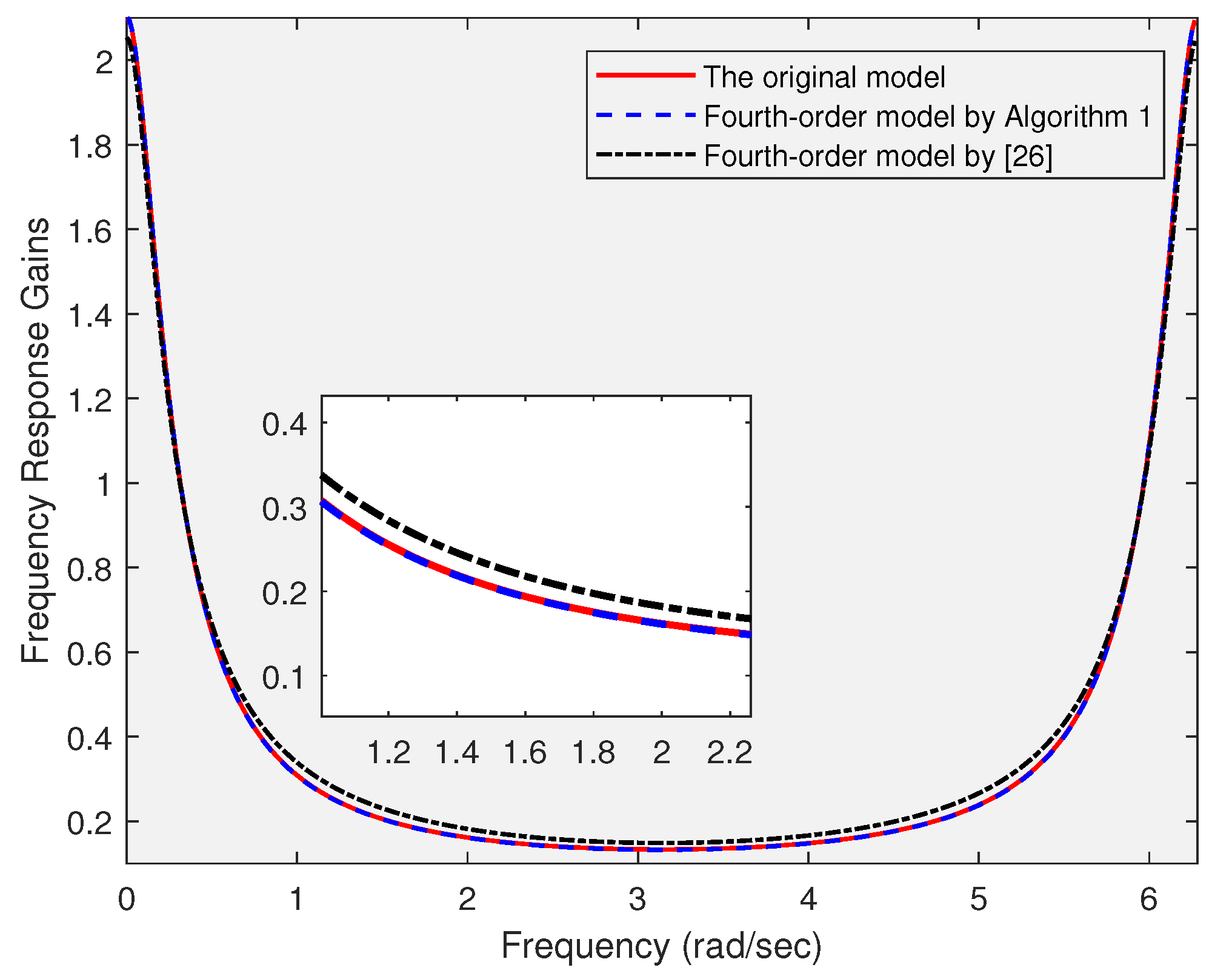
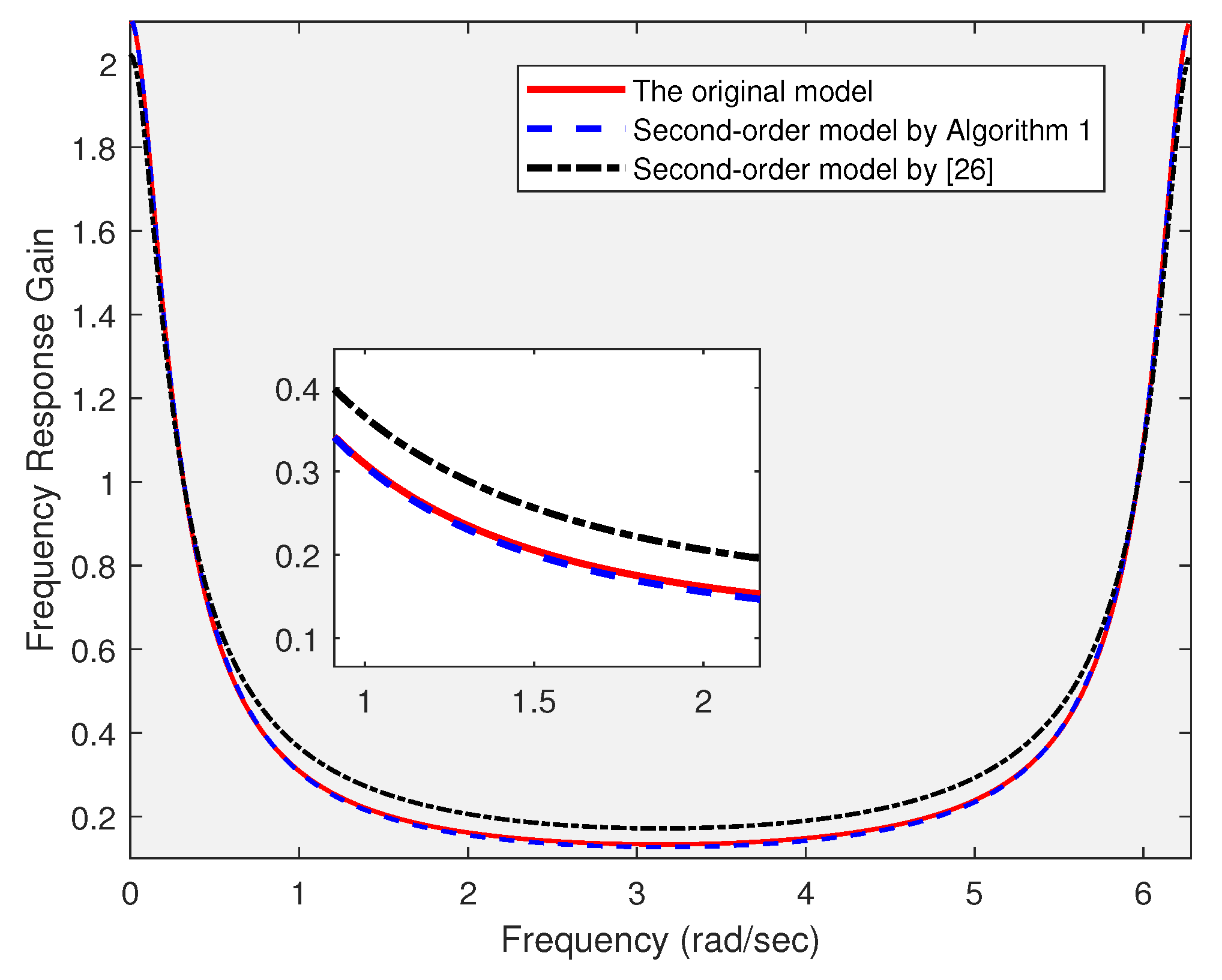
. It can be readily observed from the attained results that the provided algorithm can achieve smaller $H_{\infty }$ performance indices than [26]. To evaluate the approximation effects of different model reduction methods, Figure 1 and Figure 2 provide the frequency response gains of the original and reduced-order systems, and Figure 3 and Figure 4 depict the frequency response gains of the associated error systems with different orders. We can easily infer that compared with $G_r^{{(4)}^{\prime }}$ and $G_r^{{(2)}^{\prime }}$, the frequency gains of proposed forth-order $G_r^{(4)}$ model and second-order one $G_r^{(2)}$ are much closer to the original system, and the associated error system with $G_r^{(4)}$ and $G_r^{(2)}$ have smaller gains than that for corresponding $G_r^{{(4)}^{\prime }}$ and $G_r^{{(2)}^{\prime }}$, which illustrates the benifits of the proposed algorithm.

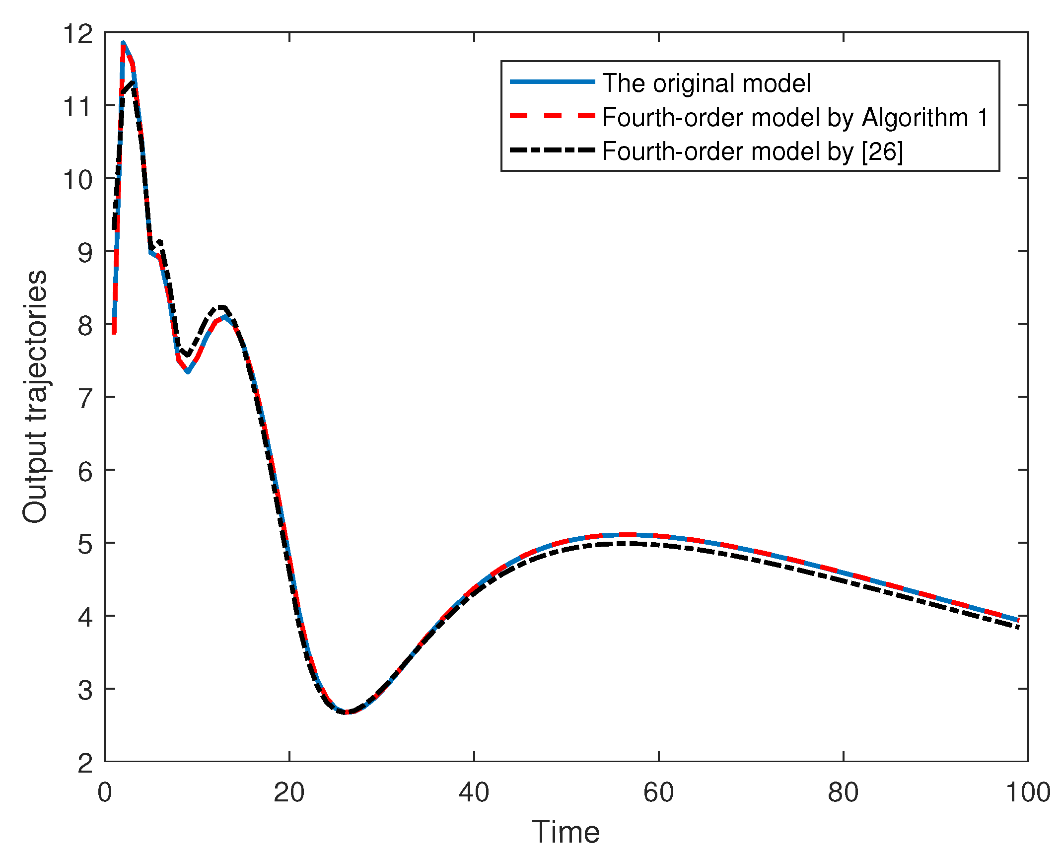
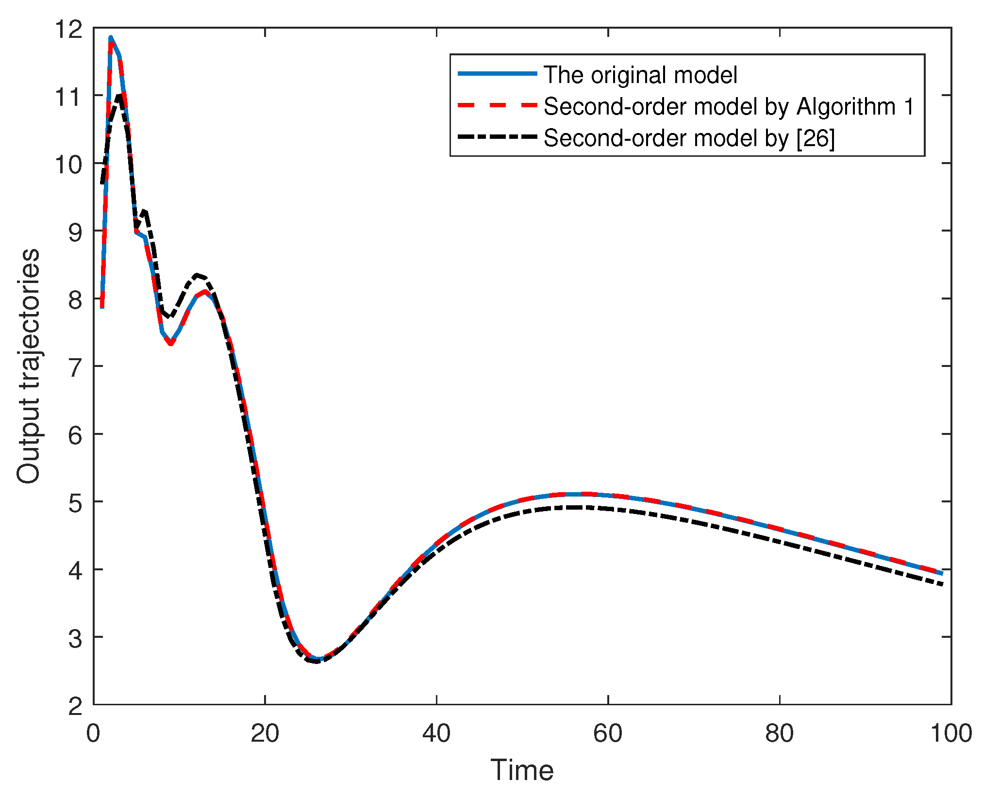
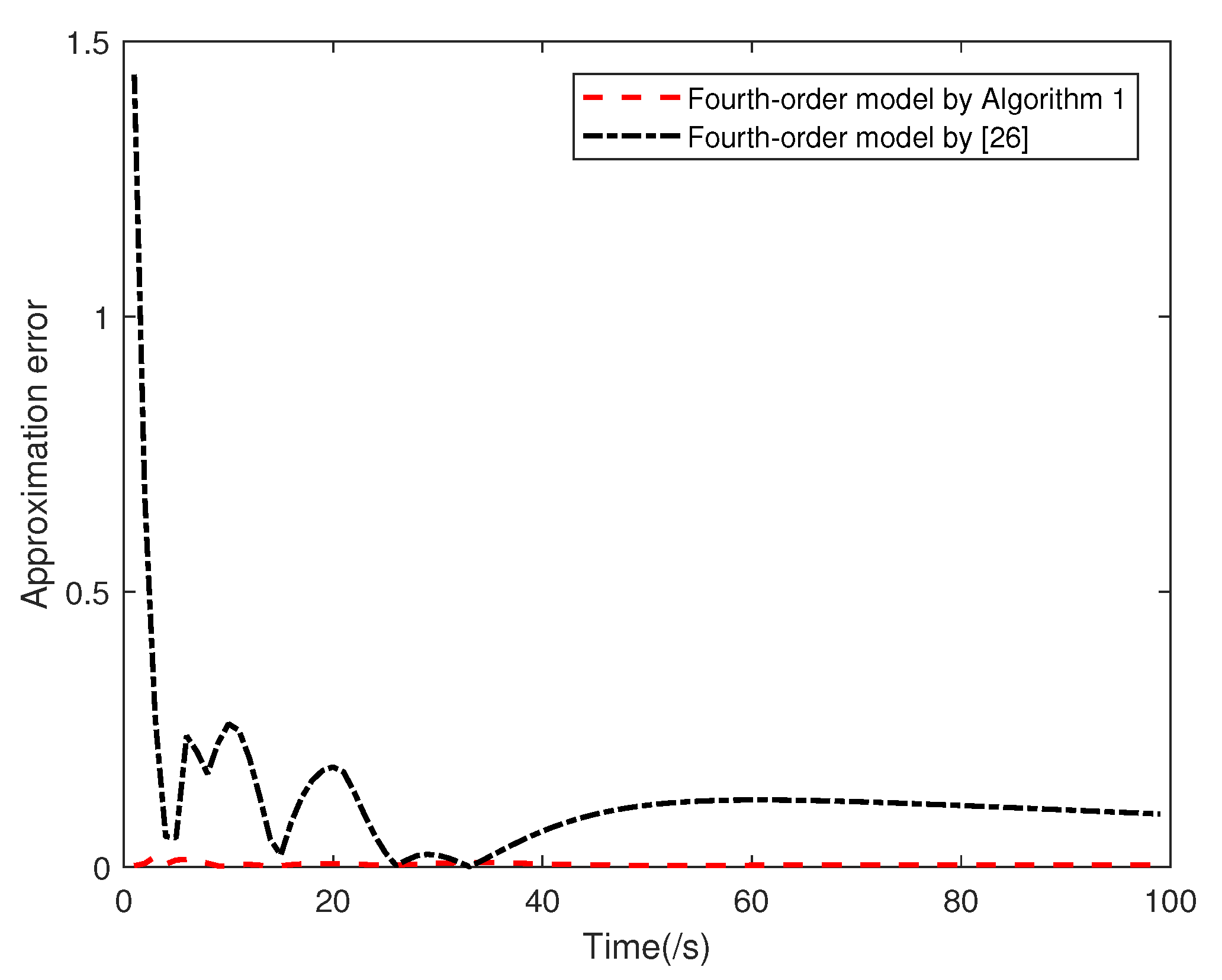
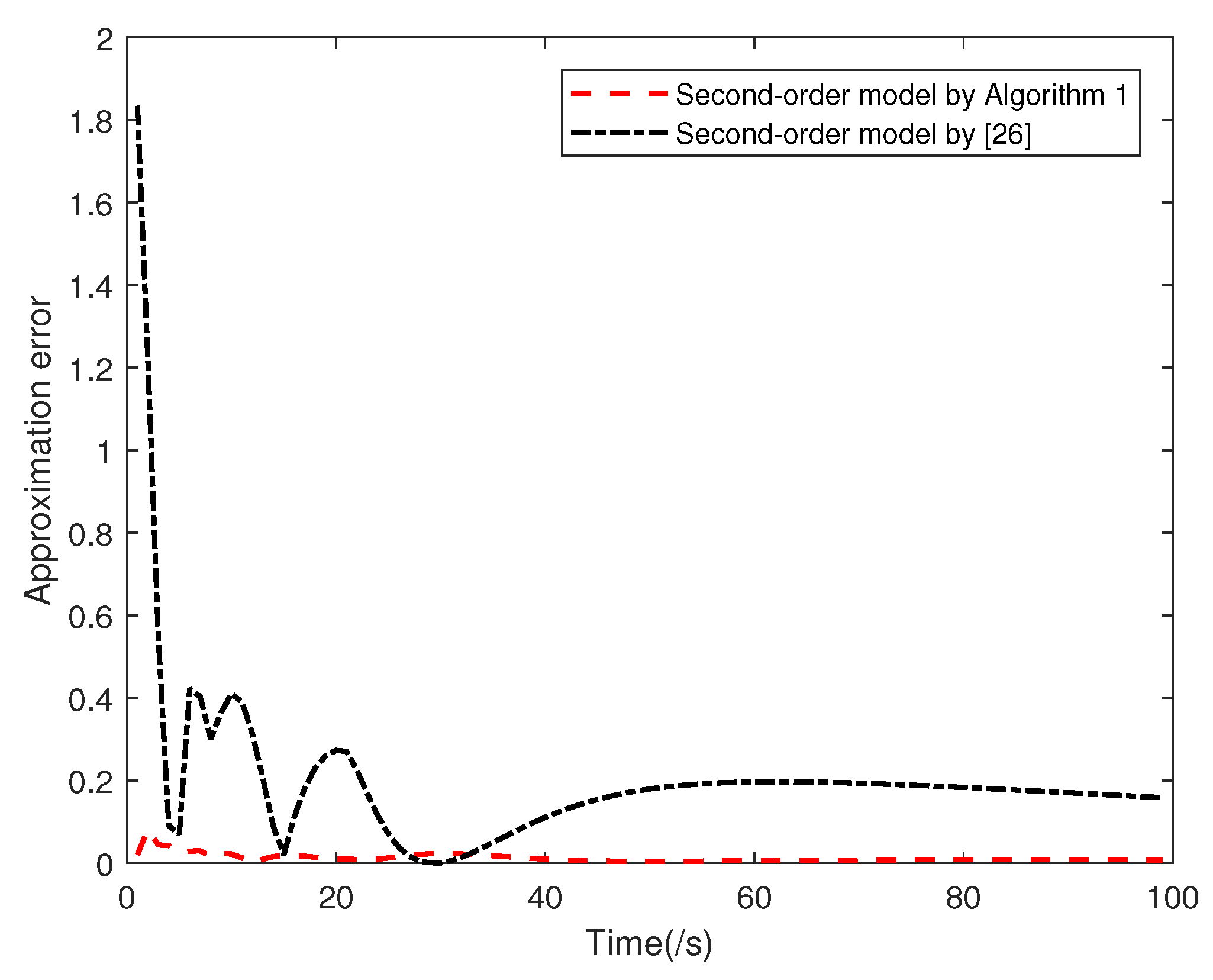
To further verify the efficiency of the obtained reduced-order models, we will show their approximation performances under the initial conditions $x(0)=\mathbf{0},x_r(0)=\mathbf{0}$ and the input

$$u(k)={\left[\begin{array}{cc}{e}^{-0.01k}|5cos(10k)|& \frac{5}{1+5k}|sin(\frac{\pi }{10}k)|\end{array}\right]}^T.$$

Figure 5 and Figure 6 depict the output trajectories of the original model and the reduced-order models with $n_r=4$ and $n_r=2$, respectively, and Figure 7 and Figure 8 show the corresponding approximation errors between the original model and the reduced-order ones. It can be seen that the proposed method can approximate the original model without causing remarkable errors.

5. Conclusions

This paper presents an $H_{\infty }$ model-reduction method that preserves positivity. In particular, the $H_{\infty }$ performance of the associated error system is characterized by BMI, and the positivity of the reduced-order model is formulated as an element-wise positivity constraint. Based on this, a sufficient condition for the existence of the desired reduced-order system has been established in the form of LMI. Furthermore, an SCO has been developed to optimize the desired reduced-order model. Finally, a compartmental network example has been provided to verify that the proposed result permits a sufficient improvement in $H_{\infty }$ performance. Future research directions are related to the static output feedback problem of complex positive systems via the proposed algorithm.

References

1. Zhu, S.; Han, Q.L.; Zhang, C. l1-gain performance analysis and positive filter design for positive discrete-time Markov jump linear systems: A linear programming approach. Automatica 2014, 50, 2098–2107. [Google Scholar] [CrossRef]
2. Shorten, R.; Wirth, F.; Leith, D. A positive systems model of TCP-like congestion control: Asymptotic results. IEEE ACM Trans. Netw. 2006, 14, 616–629. [Google Scholar] [CrossRef] [Green Version]
3. Silva-Navarro, G.; Alvarez-Gallegos, J. Sign and stability of equilibria in quasi-monotone positive nonlinear systems. IEEE Trans. Autom. Control. 1997, 42, 403–407. [Google Scholar] [CrossRef]
4. Van Den Hof, J. Positive linear observers for linear compartmental systems. SIAM J. Control. Optim. 1998, 36, 590–608. [Google Scholar] [CrossRef]
5. Berman, A.; Plemmons, R.J. Nonnegative Matrices in the Mathematical Sciences; SIAM: Bangkok, Thailand, 1994. [Google Scholar]
6. Valcher, M.E. Controllability and reachability criteria for discrete time positive systems. Int. J. Control. 1996, 65, 511–536. [Google Scholar] [CrossRef]
7. Rantzer, A. On the Kalman-Yakubovich-Popov lemma for positive systems. IEEE Trans. Autom. Control. 2015, 61, 1346–1349. [Google Scholar] [CrossRef] [Green Version]
8. Knorn, F.; Mason, O.; Shorten, R. On linear co-positive Lyapunov functions for sets of linear positive systems. Automatica 2009, 45, 1943–1947. [Google Scholar] [CrossRef] [Green Version]
9. Deaecto, G.S.; Geromel, J.C. H2 State Feedback Control Design of Continuous-Time Positive Linear Systems. IEEE Trans. Autom. Control. 2016, 62, 5844–5849. [Google Scholar] [CrossRef]
10. Shen, J.; Lam, J. Static output-feedback stabilization with optimal L1-gain for positive linear systems. Automatica 2016, 63, 248–253. [Google Scholar] [CrossRef]
11. Meng, A.; Lam, H.K.; Liu, F.; Yang, Y. Membership-Function-Dependent Design of l1-Gain Output Feedback Controller for Stabilization of Positive Polynomial Fuzzy Systems. IEEE Trans. Fuzzy Syst. 2022, 30, 2086–2100. [Google Scholar] [CrossRef]
12. Xiao, S.; Ge, X.; Han, Q.L.; Zhang, Y. Distributed resilient estimator design for positive systems under topological attacks. IEEE Trans. Cybern. 2021, 51, 3676–3686. [Google Scholar] [CrossRef] [PubMed]
13. Zhang, J.; Raïssi, T.; Shao, Y.; Cai, X. Event-triggered filter design of positive systems with state saturation. IEEE Syst. J. 2021, 15, 4281–4292. [Google Scholar] [CrossRef]
14. Li, X.; Yin, S.; Gao, H. Passivity-preserving model reduction with finite frequency H approximation performance. Automatica 2014, 50, 2294–2303. [Google Scholar] [CrossRef]
15. Ibrir, S. A projection-based algorithm for model-order reduction with H2 performance: A convex-optimization setting. Automatica 2018, 93, 510–519. [Google Scholar] [CrossRef]
16. Kürschner, P. Balanced truncation model order reduction in limited time intervals for large systems. Adv. Comput. Math. 2018, 44, 1821–1844. [Google Scholar] [CrossRef] [Green Version]
17. Breiten, T.; Unger, B. Passivity preserving model reduction via spectral factorization. Automatica 2022, 142, 110368. [Google Scholar] [CrossRef]
18. Benner, P.; Ohlberger, M.; Cohen, A.; Willcox, K. Model Reduction and Approximation: Theory and Algorithms; SIAM: Bangkok, Thailand, 2017. [Google Scholar]
19. Heinkenschloss, M.; Reis, T.; Antoulas, A.C. Balanced truncation model reduction for systems with inhomogeneous initial conditions. Automatica 2011, 47, 559–564. [Google Scholar] [CrossRef]
20. Kavranoǧlu, D.; Bettayeb, M. Characterization of the solution to the optimal H model reduction problem. Syst. Control. Lett. 1993, 20, 99–107. [Google Scholar] [CrossRef]
21. Glover, K. All optimal Hankel-norm approximations of linear multivariable systems and their L-error bounds. Int. J. Control. 1984, 39, 1115–1193. [Google Scholar] [CrossRef]
22. Ren, Y.; Ding, D.W.; Li, Q.; Xie, X. Static Output Feedback Control for T–S Fuzzy Systems via a Successive Convex Optimization Algorithm. IEEE Trans. Fuzzy Syst. 2022, 30, 4298–4309. [Google Scholar] [CrossRef]
23. Back, J.; Astolfi, A. Design of positive linear observers for positive linear systems via coordinate transformations and positive realizations. SIAM J. Control. Optim. 2008, 47, 345–373. [Google Scholar] [CrossRef]
24. Li, P.; Lam, J.; Wang, Z.; Date, P. Positivity-preserving H model reduction for positive systems. Automatica 2011, 47, 1504–1511. [Google Scholar] [CrossRef] [Green Version]
25. Farina, L.; Rinaldi, S. Positive Linear Systems: Theory and Applications; John Wiley & Sons: Hoboken, NJ, USA, 2000. [Google Scholar]
26. Shen, J.; Lam, J. H model reduction for discrete-time positive systems with inhomogeneous initial conditions. Int. J. Robust Nonlinear Control. 2015, 25, 88–102. [Google Scholar] [CrossRef]
27. Rantzer, A. On the Kalman-Yakubovich—Popov lemma. Syst. Control. Lett. 1996, 28, 7–10. [Google Scholar] [CrossRef]
28. Godfrey, K. Compartmental Models and Their Application; Academic Press: Cambridge, MA, USA, 1983. [Google Scholar]
Figure 1. Frequency response gains of the original and reduced-order systems with n r = 4 .
Applsci 12 12277 g001
Figure 2. Frequency response gains of the original and reduced-order systems with n r = 2 .
Applsci 12 12277 g002
Figure 3. Frequency response gains of the associated error systems with n r = 4 .
Applsci 12 12277 g003
Figure 4. Frequency response gains of the associated error systems with n r = 2 .
Applsci 12 12277 g004
Figure 5. The output trajectories of the original model and G r ( 4 ) , G r ( 4 ) .
Applsci 12 12277 g005
Figure 6. The output trajectories of the original model and G r ( 2 ) , G r ( 2 ) .
Applsci 12 12277 g006
Figure 7. The approximation errors between the original model and G r ( 4 ) , G r ( 4 ) .
Applsci 12 12277 g007
Figure 8. The approximation errors between the original model and G r ( 2 ) , G r ( 2 ) .
Applsci 12 12277 g008