Fault-Tolerant Control of Multi-Joint Robot Based on Fractional-Order Sliding Mode

Abstract

In this paper, the problem of fault-tolerant control of actuators for multi-joint robots is studied. Aiming at the jitter problem in the design of fault-tolerant control law for conventional sliding mode controllers (SMC), a controller design method based on fractional-order sliding mode (FSMC) theory is proposed. At first, the mathematical model of the multi-joint robot is established and the fractional-order sliding mode surface is constructed according to the mathematical model. Then, the robust control law is designed based on the Lyapunov function. Finally, the experiments are carried out. Compared with the conventional sliding mode control, the experimental results show that the multi-joint robot is more stable under the control of fractional-order sliding mode, and it can achieve almost no jitter while tracking the reference. The steady-state error for joint1 and joint2 could reach 0.073 radians under the control of SMC, while it is 0.015 radians under the control of FSMC. The steady-state error data indicate that the fluctuation amplitude under FSMC is five times smaller than SMC for the end part of the multi-joint robot under actuator gain faults. The regulation time for joint1 and joint2 is about 0.11 s under the control of SMC, and it is around 0.04 s for FSMC. The regulation time is reduced to one of three or four. These data show the effectiveness of the FSMC proposed in this paper.

1. Introduction

The robot is an important achievement produced by the comprehensive development of information science, artificial intelligence science, and modern processing and manufacturing technologies in the field of automatic control [1,2]. It is widely used in various industrial fields, such as aerospace and industrial automation, and it is the object of key development and research in countries around the world. When the robot system fails, it is extremely important to design a fault-tolerant control law to ensure that the robot can perform basic control functions. Because of the complex structure and powerful functions of multi-joint robots, it is very difficult to achieve fault-tolerant control [3].

The fault-tolerant control of the robot is also divided into passive and active fault-tolerant control from the macroscopic level. The difference between the two is whether the controller is adjusted when the fault occurs [4]. For a passive fault-tolerant control system, the robust controller is designed mainly based on some prior knowledge of faults in the current system. Once the controller is designed, it will not be adjusted in real time. Active fault-tolerant control strategies may involve switching between multiple sets of control algorithms when a system fault occurs or correcting the gain of the controller according to the fault information. Considering the complexity of the multi-joint robot control system and the variety of fault types, there are few studies on the fault control of multi-joint robots using passive fault-tolerant control, and most of the existing literature uses active fault-tolerant control methods.

In terms of active fault-tolerant control of the multi-joint robot, the existing research methods can be divided into three categories, and they are data-based, redundant sensor-based, and model-based fault-tolerant control methods [5].

The data-based fault-tolerant control method does not rely on an accurate robot system model and realizes fault tolerance by utilizing a large amount of online data in the process [6]. As the structure of the industrial robots gradually becomes more complex, the amount of data generated by the system gradually becomes larger, so more important parameters need to be fed back, which adversely affects the design of the controller. Therefore, the fault-tolerant control method based on pattern recognition is proposed. Under the premise that it is impossible to establish an accurate mathematical model of a multi-joint robot, the pattern recognition method is used to control the robot’s fault tolerance, and the typical representative is deep learning. Z. Li [7] developed a new model predictive control (MPC) method based on visual servos. In the presence of both kinematic and dynamic constraints, quadratic programming (QP) is used for control design, and neural dynamic optimization techniques are used to guide a wheeled mobile robot to move toward the desired target in a polar coordinate system. C. Yang [8] proposed an enhanced robot skill-learning system that considers both motion generation and trajectory tracking. It combines the Gaussian mixture model and Gaussian mixture regression to improve the learning performance of the model. S. Li [9] used the improved neural network for the position error accumulation and convex constraint problems in the existing manipulator recurrent neural network controller design, and proved the effectiveness in the position regulation and tracking control of a robot. There are still many studies on using neural network methods to realize fault-tolerant control of multi-joint robots [10,11,12]. However, the neural network method needs to use the data set to train the model in advance. M.K [13] assumes that the dynamic function of the robot is unknown, and proposes two dual adaptive neural network control schemes. The parameters of the neural network controller are estimated randomly in real time. The effectiveness of the controller in the trajectory tracking problem of a differentially driven wheeled mobile robot is verified using statistical hypothesis testing. The neural network model is used in the design process of the robot’s fault-tolerant controller, which needs to be combined with a high-performance computer to achieve decent results. Therefore, the neural network model is not suitable for the control process with high dynamic performance requirements.

The fault-tolerant control of the multi-joint robot based on additional sensors improves the stability of the robot control system by installing redundant sensors at the beginning of the design. Georgethuruthel T. [14] uses a combination of redundant and disjoint strain sensors to compensate for the time-varying hidden state of the system and achieves decent static variable estimates on pneumatic actuators. Professor Rodney Brooks of MIT has designed a class of small autonomous robot systems for outer space missions, equipped with more than sixty sensors, which brings challenges to the structural design of the system and reduces the payload of the robot [15]. Fault-tolerant control of robots based on additional sensors will increase the cost of the system and limit the development of robot miniaturization. At present, fault-tolerant control is realized by software signal processing, which has gradually become an alternative solution [16,17].

The model-based fault-tolerant control law for a robot involves the mathematical model of the robot in the design process so that it can predict what effect the control output will have on the robot system and the system parameters can be tuned accordingly. The representative of these methods includes adaptive control, optimal control, model predictive and back-stepping control, etc. [18,19,20]. Yajie Ma develops an adaptive compensation control scheme for two physically linked two-wheel-drive mobile robots with multiple actuator faults [21]. Yong Xu investigates the fully distributed observer-based adaptive fault-tolerant synchronization problem (SP) of multiagent systems with event-triggered control mechanisms [22]. Huaguang Zhang proposed an adaptive fuzzy fault-tolerant tracking control for partially unknown systems with actuator faults [23]. The main disadvantage of adaptive control is that it is difficult to ensure the global stability of the closed-loop system in the whole adaptive process. The other popular control method is optimal control. Ravi used optimal planning and control schemes for real-world robotic applications [24]. Haijun Peng researched a symplectic instantaneous optimal control for robot trajectory tracking [25]. Considering uncertainty in optimal robot control, José R. studied the stochastic optimal control problem with high-order cost statistics, which promotes the application of robots [26]. The control law of optimal theory relies heavily on the model of robots, but it is not easy to obtain an accurate model of the robot, which limits the application of optimal control. There are many other types of research involving fault tolerance control of the robots. Z. Jiang [27] used the equivalent replacement of the mass-spring-damper model for the space station robot astronauts, established a viscoelastic dynamic humanoid robot model in a microgravity environment, and initially proved its effectiveness. Y. Chen [28] combined MPC and adaptive control to study the trajectory tracking control problem of mobile robots and achieved good control results. Many other model-based multi-joint control schemes are introduced in [29,30,31]. The advantage of this type of control method is that the control effect is better and the performance can be optimized, while the disadvantage is that the mathematical model of the controlled object needs to be accurately established, and the control effect may be poor when the modelling is not accurate.

2. Related Works

So far, the fault-tolerant control of multi-joint collaborative robots is still divided into two types and they are model-free and model-based control law design methods, of which proportional–integral–derivative (PID) control and MPC still account for the majority. The above two methods are typical representatives of model-free and model-based fault-tolerant control laws, respectively. Generally, PID controller parameters are difficult to adjust, the parameter margin of the controller is difficult to obtain, and the dynamic process cannot be accurately controlled [32]. As for MPC, theoretically, there is still no clear explanation for the stability of closed-loop systems. Data-driven fault-tolerant control has become a research hotspot in recent years, but the computational complexity and the application cost of this method are much higher than those of other methods. For the fault-tolerant control of multi-joint robots, advanced control algorithms still need to be studied. Sliding mode control has a strong application prospect in the fault-tolerant control of multi-joint collaborative robots because the design process of the control law is based on the controlled object model, but does not rely on it strongly [33,34,35].

Mien Van [36] uses a fast non-singular terminal sliding mode controller for the fault-tolerant control of the manipulator’s arm. The proposed controller can keep the integral non-singular fast terminal sliding mode control in high robustness, fast transient response, and finite time convergence advantages. However, its disadvantage is that the proposed non-singular fast terminal sliding mode control law design process relies on the prior knowledge of disturbance and uncertainty thresholds, for which it is necessary to use adaptive technology to estimate the upper limit of the disturbance. Huiming Wang [37] studied the problem that the flexible actuators of flexible multi-joint collaborative robots cannot guarantee high tracking performance under the condition of mismatched interference using continuous sliding mode control, and it adopts the generalized proportional-integral observer technique and designs a new sliding surface based on the disturbance estimation to deal with the adverse effects of matching/mismatching time-varying disturbances. There are still many studies on the control of multi-joint collaborative robots using conventional low-order sliding modes. As the sliding surface of the low-order sliding mode design is linear, the performance is difficult to guarantee [33,34]. The design of a high-order sliding mode controller gradually enters the field of robot fault-tolerant control [36,38]. Although the high-order sliding mode can make the control input continuous, it avoids the occurrence of high gain switching, so that the chattering phenomenon of the low-order sliding mode control can be suppressed. However, the high-order sliding mode also has shortcomings. For example, it requires the prediction of the upper bound of the uncertainty of the robot system. There are still many difficulties in the parameter selection of the high-order sliding mode [39].

Considering the drawbacks of the existing SMC applied to robot control under actuator fault, in this paper, the FSMC is proposed and well designed. The main innovations are summarized as follows, compared with common regular SMC.

(1) The fractional differential operator is introduced into the sliding mode surface design process. From the perspective of the complex frequency domain, the differential operator has the advantage of phase lead; thus, the response time is reduced. The realization of the differentiation operation involves summation, so the ripples in the output voltage of the controller are eliminated.

(2) The FSMC controller is designed and its robustness and stability are guaranteed by the Lyapunov function, so the controller can handle a variety of serious conditions, such as actuator constant gain fault and constant deviation fault. This can be seen in the experiment section.

(3) Comparative experiments were carried out to compare with the conventional sliding mode in terms of trajectory tracking error and control voltage ripple. The result shows that there are fewer ripples in the controller output voltage, so the ripple torque is reduced, which helps to improve the lifespan of the robot.

3. Fractional-Order Sliding Mode Controller Design

Before introducing the design process of fractional-order sliding mode control law, the basic notation of fractional calculus is given below.

$$D_t^{\alpha }=\left\{\begin{array}{ll}\frac{d^{\alpha }}{d{t}^{\alpha }}& ,\alpha >0\\ 1& ,\alpha =0\\ {\displaystyle \underset{0}{\overset{\tau }{\int }}{(d\tau )}^{-\alpha }}& ,\alpha <0\end{array}\right.$$

(1)

In the above formula, $D_t^{\alpha }$ is called an arbitrary-order differential operator. There is no unified solution for the value of $\alpha$. The three most representative solutions are given by GrunwaldLetnikov (GL), RiemannLiouville (RL), and Caputo [40]. From a control and signal processing perspective, GrunwaldLetnikov expresses fractional calculus by summing terms, so it is intuitive to implement using digital signal controllers. When RiemannLiouville defines fractional calculus where the Laplace transform is performed, the initial value of n fractional derivatives of the function at the initial moment needs to be known. For the actual system, limited by the still vague concept of fractional calculus, it is very difficult to obtain the initial value of n fractional derivatives at zero time. The Caputo fractional operation scheme of order only needs to know the initial value of the integer derivative, and the integer derivative has a clear physical meaning, so it is widely used in practice and its expression is as follows.

Definition 1

([41]). $\alpha$-order Caputo fractional operation scheme is defined as follows.

$$D_t{}^{\alpha }f(t)=\frac{1}{\mathsf{\Gamma }\left(n-\alpha \right)}{\displaystyle {\int }_{t_0}^t\frac{f^n\left(\tau \right)}{{\left(t-\tau \right)}^{\alpha +1-n}}d\tau }$$

(2)

In the above formula, $n-1<\alpha <n,n\in Z^{+}$, $\mathsf{\Gamma }(n-\alpha )$ is the gamma function and the calculation expression is as follows.

$$\mathsf{\Gamma }\left(x\right)={\displaystyle {\int }_0^{\infty }{y}^{x-1}}{e}^{-y}dy,x>0$$

(3)

It can be seen from the above formula that one of the differences between fractional calculus and integer calculus is that fractional calculus is related to the historical state information of the system. The fractional calculus operator $D_t{}^{\alpha }f(t)$ is global, but the integer calculus is only related to the information of a limited number of points. Therefore, fractional calculus can achieve a more complete description of the historical process of the model.

When designing a controller using fractional-order sliding mode theory, it must be ensured that the system is asymptotically stable when it approaches the sliding mode surface. Usually, Lemma 1 is used to judge whether the system is stable or not.

Lemma 1

([42]). Assuming that the state $x=0$ is the equilibrium point of the fractional non-autonomous system, the fractional differentiation of the system state is written as

$$D_t{}^{\alpha }x(t)=f\left(x,t\right)$$

(4)

The function $f\left(x,t\right)$ in the above formula needs to satisfy the Lipschitz condition.

Supposing that there is a Lyapunov function $V\left(t,x(t)\right)$ such that the following formula holds

$$\left\{\begin{array}{l}{a}_1‖x‖\le V\left(t,x\right)\le a_2‖x‖\\ \dot{V}\left(t,x\right)\le -a_3‖x‖\end{array}\right.$$

(5)

In Equation (5) $a_1,$ $a_2,$ and $a_3$ are all coefficients greater than zero; the system described by Formula (4) is said to be asymptotically stable. Usually, considering that the coefficients $a_1,a_2,a_3$ are difficult to obtain, Lemma 2 is often used to judge whether the origin is asymptotically stable.

Lemma 2

([42]). For a given continuous function $\dot{x}=f\left(x\right)$, $f(0)=0$ and $x\in R,$ if there is a continuous positive definite function $V:R^n\to R,a\in R^{+},\beta \in \left(0,1\right)$ and there is a neighborhood $U_0\subseteq R^n$ of the origin such that the following formula holds

$$\dot{V}\left(x\right)+a{V}^{\beta }\left(x\right)\le 0,x\in U_0/\left\{0\right\}$$

(6)

Then the origin is an equilibrium point, where the system states can be reached in a finite time.

3.1. Multi-Joint Robot Model

This paper takes a double-joint manipulator as an example, and its physical equivalent model is shown in Figure 1.

Two joint position angles $q_1$ and $q_2$ are selected as state variables. According to Lagrange’s theorem, the dynamic equation of the above double-joint manipulator can be obtained as follows [42].

$$M(q)\ddot{q}+B(q,q)\dot{q}+G(q)=T+\omega$$

(7)

In Formula (7), $q={\left[q_1,q_2\right]}^T$ is the state variable of the double-joint manipulator, which represents the angle of the joint arm relative to the horizontal axis. $G\left(q\right)$ is the gravity term, $\omega$ is the external disturbance. $M\left(q\right),$ $B\left(q,\dot{q}\right),$ and $G\left(q\right)$ are the positive definite mass matrix, Coriolis force matrix, and gravity term, respectively. The calculation expressions are as follows.

$$\left\{\begin{array}{l}M\left(q\right)=\left[\begin{array}{cc}v+q_{01}+2q_{02}\cos (q_2)& q_{01}+q_{02}\cos (q_2)\\ q_{01}+q_{02}\cos (q_2)& q_{01}\end{array}\right]\\ B\left(q,\dot{q}\right)=\left[\begin{array}{cc}-q_{02}{\dot{q}}_2\sin \left(q_2\right)& -q_{02}({\dot{q}}_1+{\dot{q}}_2)\sin \left(q_2\right)\\ q_{02}{\dot{q}}_1\sin \left(q_2\right)& 0\end{array}\right]\\ G(q)=\left[\begin{array}{c}15g\cos (q_1)+8.75g\cos (q_1+q_2)\\ 8.75g\cos (q_1+q_2)\end{array}\right]\end{array}\right.$$

(8)

where parameter $v=13.3$ is the item relative to the connector of joint1, $q_{01}=8.98$ is the item relative to the connector of joint2, $q_{02}=8.75$ are constants related to the joint mass and length, and $g=9.8\mathrm{m}/{\mathrm{s}}^2$ is the gravitational acceleration.

3.2. Design of Fractional-Order Sliding Mode Controller for Multi-Joint Robots

When common faults occur in the actuators of multi-joint robots, such as constant gain and constant deviation faults, the actuators are not completely damaged at this time, so the fractional-order sliding mode control method can be used to design the controller to achieve fault-tolerant control.

In the design of fractional-order sliding mode control law, consider $q_d={\left[q_{d1},q_{d2}\right]}^T$ as the reference of the double joints, $e={\left[q_d-q\right]}^T$ as the error signal matrix, and $q={\left[q_1,q_2\right]}^T$ as the position angle, which is the system state variable.

The sliding mode surface for SMC is set $S_1=\dot{e}+e$, choosing the Lyapunov function $V_1$ with the following format.

$$V_1=\frac{1}{2}{S}_1^T{S}_1$$

(9)

The SMC control law $T_1$ could be deduced as follows.

$$T_1=M\left[{\ddot{q}}_d+\dot{e}+sign\left(S_1\right)\right]+B·\dot{q}+G$$

(10)

The fractional-order sliding mode surface is designed as follows.

$$S_2=\dot{e}+Ce+D_t{}^{\alpha }e$$

(11)

By choosing the constant matrix $C=\left[\begin{array}{cc}20& 0\\ 0& 20\end{array}\right]$, derivation of the above formula can be obtained as

$$\begin{array}{ll}\hfill {\dot{S}}_2& =D_t{}^{\alpha -1}e+C\dot{e}+\ddot{e}\\ & =D_t{}^{\alpha -1}\left(q_d-q\right)+C\dot{e}+\left({\ddot{q}}_d-\ddot{q}\right)\end{array}$$

(12)

In the design process of the sliding mode controller, the reaching law needs to be designed. The design of the reaching law is varied, and the symbol function $-k\mathrm{sgn}(s)$ is often used as the design criterion. Considering the chattering problem caused by the sign function, the chattering phenomenon exists when the state of the manipulator is switched near the sliding mode surface. In this paper, the hyperbolic tangent function is used instead of the $sign$ function, and the designed reaching law $T_2$ is as follows.

$$\begin{array}{ll}{T}_2& =M\left(q_d^{(\alpha -1)}+C\dot{e}+{\ddot{q}}_d\right)+B\left(q_d^{\left(\alpha \right)}+Ce+{\dot{q}}_d\right)+K(q^{(\alpha +1)}+q)\\ & -\omega +\mathsf{\Gamma }\left(e\right)\tanh (S_2)\end{array}$$

(13)

where $K$ is the converge matrix and its value was chosen as $5\ast I_{2\times 2}$, where $I_{2\times 2}$ is the identity matrix of dimension $2\times 2$. $\mathsf{\Gamma }\left(·\right)$ is the gamma function. In the algorithm implementation process, the torque has multiplied by a coefficient $\rho ,0<\rho <1$, and then added with the offset value $T_{off}$ to simulate actuator gain and deviation fault. In the simulation section, $\rho$ switches between 20%, 40%, and 60%, while $T_{off}$ gets its value among 50 $\mathrm{N}·\mathrm{m}$, 100 $\mathrm{N}·\mathrm{m}$, 200 $\mathrm{N}·\mathrm{m}$ and 300 $\mathrm{N}·\mathrm{m}$.

3.3. Proof of Stability

In order to verify whether the multi-joint robot controlled by the fractional-order sliding mode control law is stable, it is necessary to analyze the stability theoretically. Compared with classical calculus, fractional calculus faces two major problems, namely, non-locality and weak singularity, which makes the research of fractional calculus very difficult. It is also the root cause of the difficulty in the stability analysis of practical problems using fractional calculus indirectly. Therefore, in this paper, the stability of the fractional-order sliding mode controller is verified by the Lyapunov function from the perspective of energy.

Set the following Lyapunov function as

$$V_2=\frac{1}{2}{S}_2{}^T{I}_{2\times 2}{S}_2$$

(14)

where $I_{2\times 2}$ is a positive definite constant matrix. The derivative of the above formula is

$$\begin{array}{ll}{\dot{V}}_2& =\frac{1}{2}{S}_2{}^T{\dot{I}}_{2\times 2}{S}_2+S_2{}^T{I}_{2\times 2}{\dot{S}}_2\\ & =S_2{}^T{I}_{2\times 2}{\dot{S}}_2\\ & =S_2{}^T{I}_{2\times 2}\left[D_t{}^{\alpha -1}e+C\dot{e}+\ddot{e}\right]\\ & =S_2{}^T{I}_{2\times 2}\left[D_t{}^{\alpha -1}\left(q_d-q\right)+C\left({\dot{q}}_d-\dot{q}\right)+\left({\ddot{q}}_d-\ddot{q}\right)\right]\end{array}$$

(15)

The output torque vector is contained in $\ddot{q}$ item, and the torque should keep ${\dot{V}}_2$ negative at non-origin state.

As $I_{2\times 2}$ is the identity matrix and combines Formula (13), the following inequality is established.

$$\begin{array}{ll}{\dot{V}}_2& =S_2{\dot{S}}_2\\ & =S_2\left(D_t{}^{\alpha -1}\ddot{e}+C\dot{e}+\ddot{e}\right)\\ & =S_2\left(D_t{}^{\alpha -1}\left(-C{D}_t{}^{1-\alpha }\dot{e}-\epsilon D_t{}^{1-\alpha }\tanh \left(S_2\right)-D_t{}^{1-\alpha }k{S}_2\right)+C\dot{e}+\left(-C{D}_t{}^{1-\alpha }\dot{e}-\epsilon D_t{}^{1-\alpha }\tanh \left(S_2\right)-D_t{}^{1-\alpha }k{S}_2\right)\right)\\ & \le -k{S}_2{}^2-\epsilon \left|S_2\right|\\ & \le 0\end{array}$$

(16)

According to Lemma 1, the origin is the equilibrium point of the system and is asymptotically stable.

4. Simulation and Experimental Results

This part takes the actuator fault-tolerant control of a multi-joint robot as an example and mainly divides the fault types into two categories, namely, constant gain fault and constant deviation fault. The dual-joint manipulator model is established in MATLAB, and the common sliding mode and fractional-order sliding mode fault-tolerant control models are designed, respectively.

4.1. Control Block

The control block diagram is shown in Figure 2. Figure 2a is the proposed FSMC system diagram and Figure 2b is the regular SMC, which is the comparison of this article. As in regular SMC, the serial differential items $d/dt$ do not exist compared with FSMC. The differential operator has the function of phase lead, which could improve the response time.

It should be noted that the control law of FSMC is expressed in (11), and for regular SMC, it is (10).

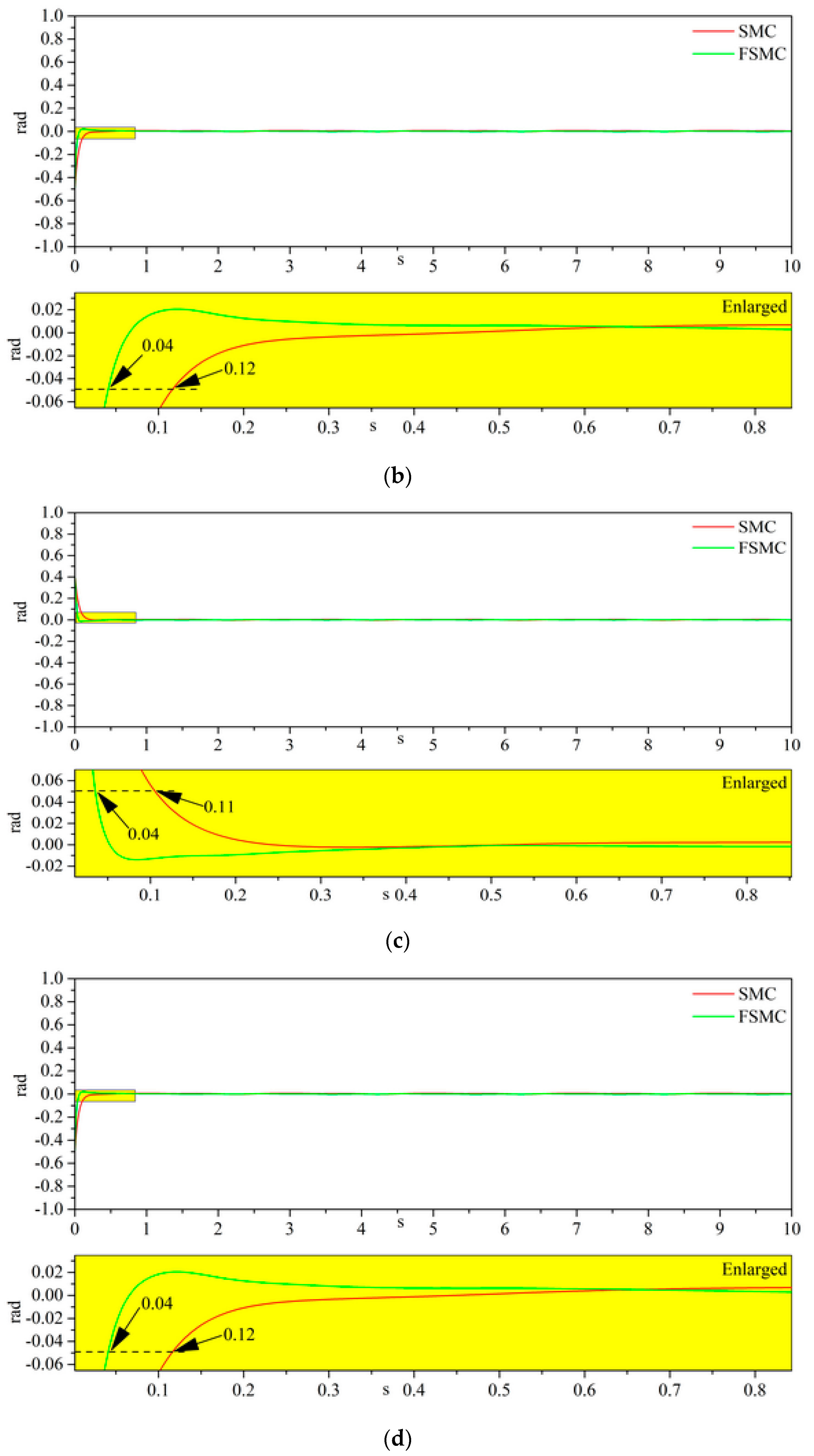
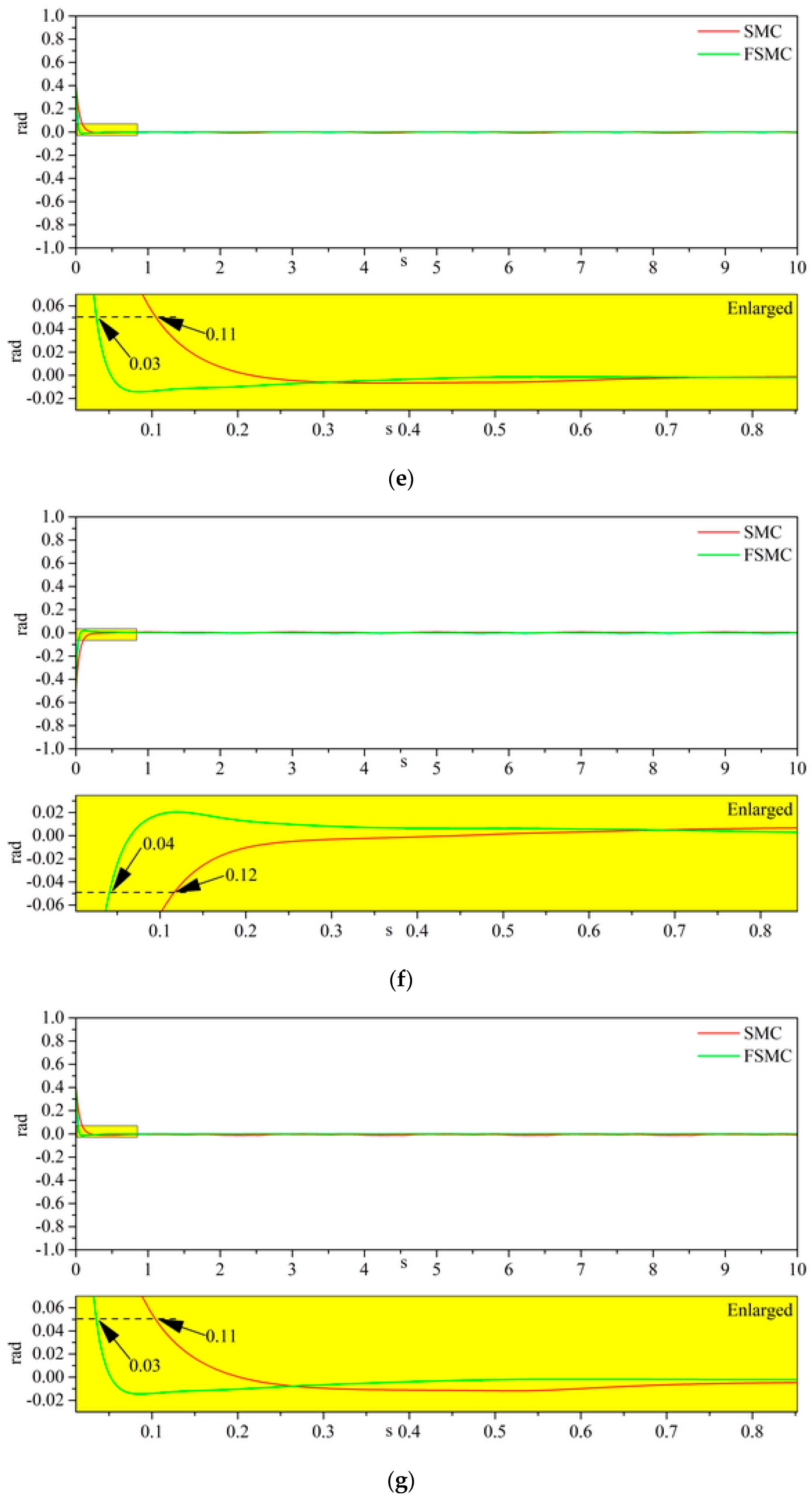
4.2. Simulation Results

The position command of joint1 is $\cos (\pi t)$, and for joint2, it is $\sin (\pi t)$, assuming that the multi-joint manipulator actuator has the constant gain failure, and the degree of constant gain failure (CGF) is 60%, 40%, and 20% of the rated value, respectively. Under the above conditions, the dynamic response curves of tracking error for both joints under different gain states are obtained. The simulation waveforms are shown in Figure 3, where the yellow figure under each figure is the enlarged part corresponding to the original figure.

Figure 3 shows the simulation results corresponding to the actuator constant gain fault. The first thing we know from Figure 3a,b is that the fluctuation exists during the tracking process using SMC, and as the CGF decreases from 60 percent to 20 percent, the fluctuation amplitude drops from 0.073 radian to 0.017 radian for both joints. From Figure 3a–f, it is obvious that the control effect under SMC is unsatisfactory, where the fluctuation is its drawback. When the controller is changed to FSMC as proposed in this article, the fluctuation disappears.

Another simulation phenomenon could be seen from Figure 3a,b, that there is vibration during the transition stage of starting under the control of FSMC. As it can be seen, when the CGF was 60 percent, the error of joint1 converged to zero rapidly once the simulation was started, and then vibrated for three periods and then tend to be stable. A possible explanation is that the FSMC provides stronger control output, so the response time is reduced, and the manipulator state tends to be stable which is guaranteed by the Lyapunov function.

The response time difference of FSMC and SMC under different CGF is not large, as the controller only needs to compensate the gain of the broken actuator.

Combining

Table 1. Maximum errors (rad) at steady state.

		CGF 60%	CGF 40%	CGF 20%
SMC	Joint1	0.073	0.031	0.017
	Joint2	0.074	0.033	0.018
FSMC	Joint1	0.007	0.002	0.001
	Joint2	0.015	0.006	0.001

and Figure 3, it is obvious that the tracking error of the joints under the control of FSMC is reduced about ten times for joint1 and around five times for joint2. Additionally, the periodic vibration disappears by adopting FSMC, which could be due to the fractional differential operator, where the integration operation reduces the steady error. The result shows the advantage of the FSMC in the joint actuator constant gain fault.

The constant deviation fault (CDF) of the joint actuator is also studied separately; the fault degree is from 50 $\mathrm{N}·\mathrm{m}$ to 300 $\mathrm{N}·\mathrm{m}$, and the trajectory tracking error curve of the end of the double-joint manipulator is taken out, as shown in Figure 4.

Figure 4 shows the simulation results corresponding to the actuator constant deviation fault. It is easy to know from Figure 3a,b and Figure 4a,b that the vibration disappears under CDF. It can be interpreted that the constant offset fault does not change during the whole process, which is not similar with CGF, so the effect of CDF at steady state is minor. We also know from Figure 4a–f that the regulation time for both SMC and FSMC under CDF remains unchanged. Additionally, the steady-state error, if given adequate time, reaches zero, but the FSMC has the priority in the rapidity. The priority can be due to the fractional operator, in which the integration calculation can speed up the converging process.

The dotted line in Figure 4 is the boundary of five percent error zone, and the corresponding time that errors first go beyond this line is shown in

Table 2. Comparison table of maximum time (s) of dynamic error in different CDF.

		$\mathbf{CDF}50\mathbf{N}·\mathbf{m}$	$\mathbf{CDF}100\mathbf{N}·\mathbf{m}$	$\mathbf{CDF}200\mathbf{N}·\mathbf{m}$	$\mathbf{CDF}300\mathbf{N}·\mathbf{m}$
SMC	Joint1	0.11	0.11	0.11	0.11
	Joint2	0.12	0.12	0.12	0.12
FSMC	Joint1	0.04	0.04	0.03	0.03
	Joint2	0.04	0.04	0.04	0.04

.

From Table 2, it is very easy to see that the FSMC is about three times faster than the SMC in terms of joint position response time, but the steady-state error of the conventional sliding mode is close to that of the fractional-order sliding mode. Combining Figure 4 and Table 2, we can conclude that the actuator constant offset fault has nearly no effect on the response time and steady-state error. Furthermore, from Figure 3 and Figure 4, we can know that the offset fault of the actuator has more influence than the gain error in steady-state error, from which it could be interpreted that the gain fault of the actuator could be compensated by the gain design in FSMC and SMC controller, while the offset fault is eliminated by increasing the regulation time.

According to the simulation results under constant gain and constant deviation situations for the double-joint manipulator, the fractional-order sliding mode has obvious advantages for the gain or deviation fault in a wide range of fault amplitude. In particular, it has obvious advantages in improving the response speed of the multi-joint manipulator and reducing the steady-state error. In particular, the greater the degree of failure is, the more prominent the advantages of FSMC can be.

A hardware experimental platform is built to investigate the control laws of FSMC and SMC. The platform is shown in Figure 5.

Two experiments under extreme situations are investigated here. The first one is the constant gain failure with 80% output torque, and the other one is constant deviation fault where 300 $\mathrm{N}·\mathrm{m}$ of the loss is included. The oscilloscope is used to capture the experiment data.

Figure 6 shows the output voltage waveform of the double-joint manipulator using SMC and FSMC where the output torque of the joint actuator is only 80% of the rated value.

Figure 6 shows that under the condition of large actuator constant gain fault, the output voltage amplitudes of the conventional sliding mode and fractional-order sliding mode controllers are similar in steady state. However, the output voltage of the fractional sliding mode has a fluctuation of about 10 V in amplitude. Furthermore, the voltage waveforms of the FSMC and SMC when the joint actuator has a constant deviation fault are shown in Figure 7.

Figure 7 shows that under the condition of large actuator constant deviation fault, the output voltage amplitudes of the conventional sliding mode and fractional-order sliding mode controller are similar in steady state. However, the output voltage of the fractional sliding mode has a fluctuation of about 20 V in amplitude.

From comprehensive analysis of Figure 6 and Figure 7, combined with the steady-state position error curve (shown in Figure 3 and Figure 4), it can be summarized that since the differential operator is introduced in the design process of the fractional sliding mode controller, the voltage waveform shows fluctuation, which uses the phase advance effect of the differential operator to ensure the fast tracking of the joint to the reference. The comparative experiments show the superiority of FSMC in terms of rapidity and steady error characteristics.

5. Conclusions

In this paper, the problem of actuator fault-tolerant control of multi-joint robots is studied; in particular, the fault-tolerant control of actuators under constant gain fault and constant deviation fault. The novel FSMC is designed to reduce the steady-state error under sinusoidal references. Additionally, the response speed is improved under step reference compared with SM. The following conclusions can be made from the experiment results.

(1) The output voltage of the FSMC is smooth and there is no fluctuation compared with regular SMC method. There are two reasons to interpret this: the first reason is the introduction of tanh function, while the other reason is the fractional differential operator in the FSMC controller.

(2) The response time under step reference is reduced and the control accuracy under sinusoidal reference are greatly improved, where the response time under CDF is improved by three times and the maximum error under CGF is improved by ten times.

(3) The FSMC is robust under different actuator CDF and CGF, and it can achieve smooth tracking at steady state, which is superior to regular SMC.

The comparative experiments show the superiority of FSMC in terms of rapidity and steady error characteristics. Future research work could be focused on the control problem of mixed faults, so the mathematic model of the multi-joint robot needs to be simplified and tested. New control theories research applied to robots is also worth its way.

References

1. Kim, J.H. Multi-Axis Force-Torque Sensors for Measuring Zero-Moment Point in Humanoid Robots: A Review. IEEE Sens. J. 2020, 20, 1126–1141. [Google Scholar] [CrossRef]
2. Burgner-Kahrs, J.; Rucker, D.C.; Choset, H. Continuum Robots for Medical Applications: A Survey. IEEE Trans. Robot. 2015, 31, 1261–1280. [Google Scholar] [CrossRef]
3. Urrea, C.; Kern, J. Fault-Tolerant Controllers in Robotic Manipulators. Performance Evaluations. IEEE Lat. Am. Trans. 2013, 11, 1318–1324. [Google Scholar] [CrossRef]
4. Sanket, N.J.; Singh, C.D.; Ganguly, K.; Fermüller, C.; Aloimonos, Y. GapFlyt: Active Vision Based Minimalist Structure-Less Gap Detection for Quadrotor Flight. IEEE Robot. Autom. Lett. 2018, 3, 2799–2806. [Google Scholar] [CrossRef] [Green Version]
5. Khalastchi, E.; Kalech, M. Fault Detection and Diagnosis in Multi-Robot Systems: A Survey. Sensors 2019, 19, 4019. [Google Scholar] [CrossRef] [Green Version]
6. Shi, C.; Yang, G.; Li, X. Data-Based Fault-Tolerant Consensus Control for Uncertain Multiagent Systems Via Weighted Edge Dynamics. IEEE Trans. Syst. Man Cybern. Syst. 2017, 49, 2548–2558. [Google Scholar] [CrossRef]
7. Li, Z.; Yang, C.; Su, C.; Deng, J.; Zhang, W. Vision-Based Model Predictive Control for Steering of a Nonholonomic Mobile Robot. IEEE Trans. Control. Syst. Technol. 2016, 24, 553–564. [Google Scholar] [CrossRef]
8. Yang, C.; Chen, C.; He, W.; Cui, R.; Li, Z. Robot Learning System Based on Adaptive Neural Control and Dynamic Movement Primitives. IEEE Trans. Neural Netw. Learn. Syst. 2019, 30, 777–787. [Google Scholar] [CrossRef]
9. Li, S.; Zhang, Y.; Jin, L. Kinematic control of redundant manipulators using neural networks. IEEE Trans. Neural Netw. Learn. Syst. 2016, 28, 2243–2254. [Google Scholar] [CrossRef]
10. Wei, H.; Dong, Y. Adaptive Fuzzy Neural Network Control for Constrained Robot Using Impedance Learning. IEEE Trans. Neural Netw. Learn. Syst. 2018, 29, 1174–1186. [Google Scholar]
11. Yang, C.; Peng, G.; Cheng, L.; Na, J.; Li, Z. Force Sensorless Admittance Control for Teleoperation of Uncertain Robot Manipulator Using Neural Networks. IEEE Trans. Syst. Man Cybern. Syst. 2019, 51, 3282–3292. [Google Scholar] [CrossRef]
12. Jiang, Y.; Wang, Y.; Miao, J.; Na, J.; Zhao, Z.; Yang, C. Composite-Learning-Based Adaptive Neural Control for Dual-Arm Robots with Relative Motion. IEEE Trans. Neural Netw. Learn. Syst. 2020, 33, 1010–1021. [Google Scholar] [CrossRef] [PubMed]
13. Bugeja, M.K.; Fabri, S.G.; Camilleri, L. Dual Adaptive Dynamic Control of Mobile Robots Using Neural Networks. IEEE Trans. Syst. Man Cybern. Part B (Cybern.) 2008, 39, 129–141. [Google Scholar] [CrossRef]
14. Thuruthel, T.G.; Hughes, J.; Georgopoulou, A.; Clemens, F.; Iida, F. Using Redundant and Disjoint Time-Variant Soft Robotic Sensors for Accurate Static State Estimation. IEEE Robot. Autom. Lett. 2021, 6, 2099–2105. [Google Scholar] [CrossRef]
15. Ferrell, C. Failure recognition and fault tolerance of an autonomous robot. Adapt. Behav. 1994, 2, 375–398. [Google Scholar] [CrossRef] [Green Version]
16. Wang, H.; Daley, S. Actuator fault diagnosis: An adaptive observerbased technique. IEEE Trans. Automat. Contr. 1996, 41, 1073–1078. [Google Scholar] [CrossRef]
17. Tao, G.; Ma, X.; Joshi, S.M. Adaptive state feedback control of systems with actuator failures. In Proceedings of the 2000 American Control Conference. ACC (IEEE Cat. No.00CH36334), Chicago, IL, USA, 28–30 June 2000; Volume 4, pp. 2669–2673. [Google Scholar] [CrossRef]
18. Zhang, L.; Liu, H.; Tang, D.; Hou, Y.; Wang, Y. Adaptive Fixed-Time Fault-Tolerant Tracking Control and Its Application for Robot Manipulators. IEEE Trans. Ind. Electron. 2022, 69, 2956–2966. [Google Scholar] [CrossRef]
19. Inoue, D.; Ito, Y.; Yoshida, H. Optimal Transport-Based Coverage Control for Swarm Robot Systems: Generalization of the Voronoi Tessellation-Based Method. IEEE Control. Syst. Lett. 2021, 5, 1483–1488. [Google Scholar] [CrossRef]
20. Ratner, E.; Bajcsy, A.; Fong, T.; Tomlin, C.J.; Dragan, A.D. Efficient Dynamics Estimation with Adaptive Model Sets. IEEE Robot. Autom. Lett. 2021, 6, 2373–2380. [Google Scholar] [CrossRef] [PubMed]
21. Ma, Y.; Cocquempot, V.; Najjar, M.E.B.E.; Jiang, B. Adaptive Compensation of Multiple Actuator Faults for Two Physically Linked 2WD Robots. IEEE Trans. Robot. 2018, 34, 248–255. [Google Scholar] [CrossRef]
22. Xu, Y.; Wu, Z.-G. Distributed Adaptive Event-Triggered Fault-Tolerant Synchronization for Multiagent Systems. IEEE Trans. Ind. Electron. 2021, 68, 1537–1547. [Google Scholar] [CrossRef]
23. Zhang, H.; Zhang, K.; Cai, Y.; Han, J. Adaptive Fuzzy Fault-Tolerant Tracking Control for Partially Unknown Systems with Actuator Faults via Integral Reinforcement Learning Method. IEEE Trans. Fuzzy Syst. 2019, 27, 1986–1998. [Google Scholar] [CrossRef]
24. Prakash, R.; Behera, L.; Mohan, S.; Jagannathan, S. Dual-Loop Optimal Control of a Robot Manipulator and Its Application in Warehouse Automation. IEEE Trans. Autom. Sci. Eng. 2022, 19, 262–279. [Google Scholar] [CrossRef]
25. Peng, H.J.; Fei, L.F.; Liu, J.G. A symplectic instantaneous optimal control for robot trajectory tracking with differential-algebraic equation models. IEEE Trans. Ind. Electron. 2019, 67, 3819–3829. [Google Scholar] [CrossRef] [Green Version]
26. Medina, J.R.; Hirche, S. Considering Uncertainty in Optimal Robot Control Through High-Order Cost Statistics. IEEE Trans. Robot. 2018, 34, 1068–1081. [Google Scholar] [CrossRef] [Green Version]
27. Jiang, Z.; Xu, J.; Li, H.; Huang, Q. Stable Parking Control of a Robot Astronaut in a Space Station Based on Human Dynamics. IEEE Trans. Robot. 2019, 36, 399–413. [Google Scholar] [CrossRef]
28. Chen, Y.; Li, Z.; Kong, H.; Ke, F. Model Predictive Tracking Control of Nonholonomic Mobile Robots with Coupled Input Constraints and Unknown Dynamics. IEEE Trans. Ind. Inform. 2018, 15, 3196–3205. [Google Scholar] [CrossRef]
29. Liao, J.; Chen, Z.; Yao, B. Model-Based Coordinated Control of Four-Wheel Independently Driven Skid Steer Mobile Robot with Wheel–Ground Interaction and Wheel Dynamics. IEEE Trans. Ind. Inform. 2019, 15, 1742–1752. [Google Scholar] [CrossRef]
30. Khadem, M.; O’Neill, J.; Mitros, Z.; da Cruz, L.; Bergeles, C. Autonomous Steering of Concentric Tube Robots via Nonlinear Model Predictive Control. IEEE Trans. Robot. 2020, 36, 1595–1602. [Google Scholar] [CrossRef]
31. Thieffry, M.; Kruszewski, A.; Duriez, C.; Guerra, T. Control Design for Soft Robots Based on Reduced-Order Model. IEEE Robot. Autom. Lett. 2019, 4, 25–32. [Google Scholar] [CrossRef]
32. Ziquan, Y.; Youmin, Z.; Bin, J. PID-type fault-tolerant prescribed performance control of fixed-wing UAV. J. Syst. Eng. Electron. 2021, 32, 1053–1061. [Google Scholar] [CrossRef]
33. Van, M.; Mavrovouniotis, M.; Ge, S.S. An Adaptive Backstepping Nonsingular Fast Terminal Sliding Mode Control for Robust Fault Tolerant Control of Robot Manipulators. IEEE Trans. Syst. Man Cybern. Syst. 2018, 49, 1448–1458. [Google Scholar] [CrossRef] [Green Version]
34. Vo, A.T.; Kang, H. A Novel Fault-Tolerant Control Method for Robot Manipulators Based on Non-Singular Fast Terminal Sliding Mode Control and Disturbance Observer. IEEE Access 2020, 8, 109388–109400. [Google Scholar] [CrossRef]
35. Van, M.; Ge, S.S.; Ren, H. Robust Fault-Tolerant Control for a Class of Second-Order Nonlinear Systems Using an Adaptive Third-Order Sliding Mode Control. IEEE Trans. Syst. Man Cybern. Syst. 2016, 47, 221–228. [Google Scholar] [CrossRef] [Green Version]
36. Wang, H.; Pan, Y.; Li, S.; Yu, H. Robust Sliding Mode Control for Robots Driven by Compliant Actuators. IEEE Trans. Control. Syst. Technol. 2018, 27, 1259–1266. [Google Scholar] [CrossRef]
37. Nguyen, V.-C.; Vo, A.-T.; Kang, H.-J. A Finite-Time Fault-Tolerant Control Using Non-Singular Fast Terminal Sliding Mode Control and Third-Order Sliding Mode Observer for Robotic Manipulators. IEEE Access 2021, 9, 31225–31235. [Google Scholar] [CrossRef]
38. Nair, R.R.; Karki, H.; Shukla, A.; Jamshidi, M. Fault-Tolerant Formation Control of Nonholonomic Robots Using Fast Adaptive Gain Nonsingular Terminal Sliding Mode Control. IEEE Syst. J. 2018, 13, 1006–1017. [Google Scholar] [CrossRef]
39. Mujumdar, A.; Tamhane, B.; Kurode, S. Observer-Based Sliding Mode Control for a Class of Noncommensurate Fractional-Order Systems. IEEE/ASME Trans. Mechatron. 2015, 20, 2504–2512. [Google Scholar] [CrossRef]
40. Xiong, L.; Wang, J.; Mi, X.; Khan, M.W. Fractional Order Sliding Mode Based Direct Power Control of Grid-Connected DFIG. IEEE Trans. Power Syst. 2017, 33, 3087–3096. [Google Scholar] [CrossRef]
41. Momeni, D. Fractional terminal sliding mode control design for a class of dynamical systems with uncertainty. Commun. Nonlinear Sci. Numer. Simul. 2012, 17, 367–377. [Google Scholar]
42. Dinh, T.X.; Thien, T.D.; Anh, T.H.V.; Ahn, K.K. Disturbance Observer Based Finite Time Trajectory Tracking Control for a 3 DOF Hydraulic Manipulator Including Actuator Dynamics. IEEE Access 2018, 6, 36798–36809. [Google Scholar] [CrossRef]
Figure 1. Double-joint manipulator model.
Applsci 12 11908 g001
Figure 2. Sliding mode control block diagram. (a) FSMC control block. (b) SMC control block.
Applsci 12 11908 g002
Figure 3. Joint tracking error curves under different CGF. (a) Tracking error of joint1 with 60% CGF. (b) Tracking error of joint2 with 60% CGF. (c) Tracking error of joint1 with 40% CGF. (d) Tracking error of joint2 with 40% CGF. (e) Tracking error of joint1 with 20% CGF. (f) Tracking error of joint2 with 20% CGF.
Applsci 12 11908 g003aApplsci 12 11908 g003b
Figure 4. Position tracking error curves of double-joint under different CDF. (a) Tracking error of joint1 with 50 N · m CDF. (b) Tracking error of joint2 with 50 N · m CDF. (c) Tracking error of joint1 with 100 N · m CDF. (d) Tracking error of joint2 with 100 N · m CDF. (e) Tracking error of joint1 with 200 N · m CDF. (f) Tracking error of joint2 with 200 N · m CDF. (g) Tracking error of joint1 with 300 N · m CDF. (h) Tracking error of joint2 with 300 N · m CDF.
Applsci 12 11908 g004aApplsci 12 11908 g004bApplsci 12 11908 g004cApplsci 12 11908 g004d
Figure 5. Robotic experimental platform.
Applsci 12 11908 g005
Figure 6. Output voltage of FSMC and SMC under constant gain fault (80%).
Applsci 12 11908 g006
Figure 7. Output voltage of FSMC and SMC control under constant deviation fault (300 N · m ).
Applsci 12 11908 g007