A Military Object Detection Model of UAV Reconnaissance Image and Feature Visualization

Abstract

Military object detection from Unmanned Aerial Vehicle (UAV) reconnaissance images faces challenges, including lack of image data, images with poor quality, and small objects. In this work, we simulate UAV low-altitude reconnaissance and construct the UAV reconnaissance image tank database UAVT-3. Then, we improve YOLOv5 and propose UAVT-YOLOv5 for object detection of UAV images. First, data augmentation of blurred images is introduced to improve the accuracy of fog and motion-blurred images. Secondly, a large-scale feature map together with multi-scale feedback is added to improve the recognition ability of small objects. Thirdly, we optimize the loss function by increasing the loss penalty of small objects and classes with fewer samples. Finally, the anchor boxes are optimized by clustering the ground truth object box of UAVT-3. The feature visualization technique Class Action Mapping (CAM) is introduced to explore the mechanisms of the proposed model. The experimental results of the improved model evaluated on UAVT-3 show that the mAP reaches 99.2%, an increase of 2.1% compared with YOLOv5, the detection speed is 40 frames per second, and data augmentation of blurred images yields an mAP increase of 20.4% and 26.6% for fog and motion blur images detection. The class action maps show the discriminant region of the tanks is the turret for UAVT-YOLOv5.

1. Introduction

Unmanned Aerial Vehicle (UAV) reconnaissance has been an important means of obtaining information in warfare, in which military object detection is one of the most important tasks since it can identify and locate objects. However, there are still some challenges in military object detection of UAV reconnaissance images. First of all, military objects from UAV image data are difficult to obtain due to confidentiality. Secondly, UAVs are susceptible to bad weather during reconnaissance, resulting in distortions, such as fog blur and motion blur, which will reduce the image contrast and image quality. It is more difficult to detect an object in the images with low contrast and low quality. Thirdly, the resolution of UAV images is usually high due to the wide reconnaissance field of UAVs, and the objects are relatively small. Moreover, the background is also extremely complex due to military camouflage, which also brings lots of difficulties. Therefore, military object detection of UAV reconnaissance images is still an open problem.

To deal with the lack of tank image databases of UAV reconnaissance, we choose three typical main battle tanks and customize the miniaturized ratio model of the tanks. Then, we build a simulation platform of UAV low-altitude reconnaissance to capture image data of the tanks in different scenes of a wild battlefield with an RGB camera. Finally, we label the tanks in the UAV image in a manual manner and construct the UAV image tank dataset (UAVT-3).

The traditional object detection algorithm usually extracts the features manually, which has a low detection accuracy. Inspired by the great success of deep learning applied in a variety of vision tasks [1], more and more Convolutional Neural Network (CNN)-based detection algorithms have recently improved the detection accuracy. The existing CNN detection algorithms can be roughly divided into two-stage algorithms [2,3,4] and one-stage [5,6,7,8,9] algorithms. In the two-stage algorithms, a series of candidate boxes were generated at the first stage, which was then classified by a CNN at the second stage. In the one-stage algorithms, the task of target box location was modeled as a regression problem directly, which only looked at the image one time with a single network.

The series of Region-based Convolutional Networks (R-CNNs) are typical two-stage detection models. R-CNN [2] is the first detection model exploring CNN to extract visual features, which also adopted supervised pre-training of large samples and domain-specific fine-tuning to avoid the over-fitting problem in training. Although R-CNN yielded a performance boost, there are lots of repeated computations in feature extraction for each candidate region. Spatial pyramid pooling networks (SPPnets) [10] were proposed to speed up R-CNN by sharing computation, which computed a convolutional feature map for the entire input image and then classified each object proposal using a feature vector extracted from the shared feature map. Fast R-CNN [3] proposed a new training algorithm to fix the disadvantages of R-CNN and SPPnets, which improved the speed and accuracy. Faster R-CNN [4] introduced a Region Proposal Network (RPN) for nearly cost-free region proposals by sharing the convolutional features with the detection network.

The You Only Look Once algorithms (YOLOs) and Single Shot multi-box Detector (SSD) are the most popular one-stage models. The first one-stage model, YOLOv1 [5], framed object detection as a regression problem to spatially separate bounding boxes and associate class probabilities. It proposed a single neural network to predict bounding boxes and class probabilities directly from the entire image in one evaluation, which can be optimized end-to-end directly. SSD [6] proposed a deep CNN-based object detector without resampling pixels or features for bounding box hypotheses, which took feature maps of different scales for detection, and directly used convolution instead of a full connection network to obtain detection results. YOLOv2 [7] proposed various improvements to YOLOv1, including batch normalization technology, a high-resolution classifier, a new backbone network, and an anchor frame mechanism. YOLOv3 [8] explored multi-scale feature maps for detection in which the feature map size was designed according to the size of the prior anchor, introduced a more powerful backbone Darknet-53, and replaced softmax by logistic regression in prediction. YOLOv4 [9] further improved the performance of YOLOv3 by introducing a series of practical skills, which took CSPDarkNet53 as the backbone network, replaced the ReLU activation function with Mish activation function, and added data augmentation skills such as CutMix, Mosaic, and label smoothing.

It is common to say that the computation complexity of two-stage algorithms is relatively higher than that of one-stage algorithms since it includes a candidate box selecting process. It is hard to meet the needs of real-time detection for UAV reconnaissance. Therefore, a one-stage algorithm is more suitable, and YOLOv5 is one of the most popular and effective one-stage object detection algorithms. However, it is not the best choice to apply YOLOv5 to object detection of UAV images directly. First of all, fog blur and motion blur are the two most common distortions for UAV reconnaissance images, which have not been considered in the original YOLOv5. The detection accuracy of the original YOLOv5 on blurred images is very low, i.e., the generation ability in practice is poor. Then, the view angle of UAV images is different from that of the common images, and the objects in the UAV image are usually small, which will also affect the performance of YOLOv5. Moreover, the explanation of the model is still an open problem. The main contributions of our work can be summarized as:

1.

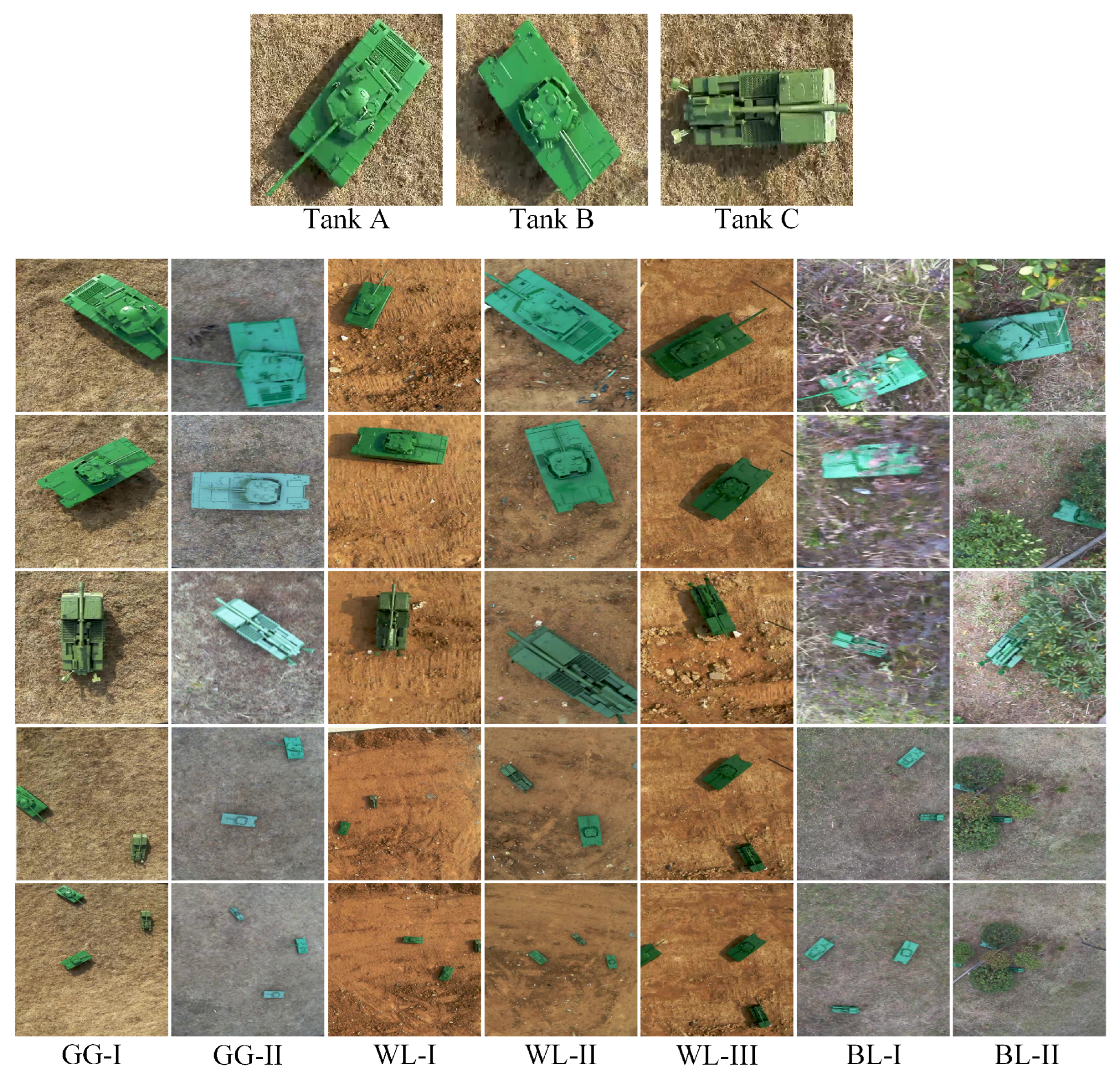
We constructed the UAV reconnaissance image tank database UAVT-3 for detection, which includes 1263 images, 7 scenes, 3 types of tanks, and 2241 marked objects.

2.

In order to improve the ability to detect small objects and blurred objects, we improved YOLOv5 by using data augmentation of blurred samples, adding a larger feature map in the neck, and optimizing the loss function and anchor priors.

3.

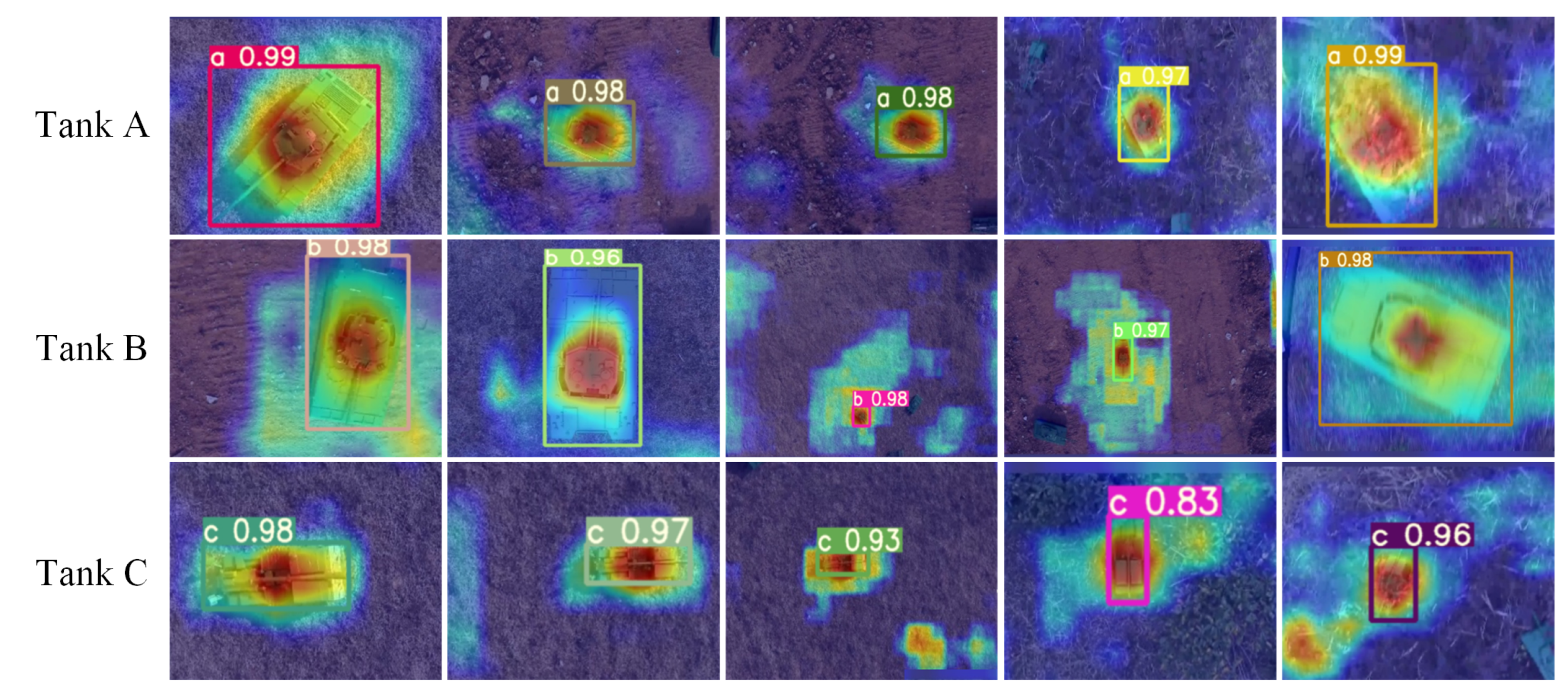
In order to improve the explanation, we introduced the feature visualization technique of Class Action Mapping (CAM) to explore the mechanism of the proposed model.

2. UAV Reconnaissance Image Tank Database

2.1. Image Capturing and Annotation

In order to collect the military object image of UAV data being close to the real battlefield scenes, we built a low-altitude reconnaissance simulation platform. First, we constructed the models of three main battle tanks according to the ratio of 10:1, marked as Tank A, Tank B, and Tank C, respectively. Seven kinds of battle scenes were simulated, which are denoted as Grass Ground I (GG-I), Grass Ground II (GG-II), Waste Land I (WL-I), Waste Land II (WL-II), Waste Land III (WL-III), Bush Land I (BL-I), and Bush Land II (BL-II), respectively. Then, we simulate the low-altitude reconnaissance scene of the UAV. One or more tanks were allocated in the simulated battlefield, and a small car equipped with an RGB camera moved on a fixed elliptical and captured the images of the tanks. It aims to simulate the UAV reconnaissance of military objects on the ground from different angles at a certain height. Then we simulated UAV reconnaissance at different heights by adjusting the track height. The simulated height $H_S$ can be obtained by

$$H_S=(S_T/S_M)\times H_T,$$

(1)

where $S_T$ and $S_M$ denote the size of the tank and its model, and $H_T$ denotes the track height. Figure 1 shows some examples of the collected images, and 1263 images were finally selected.

Next, the collected images were annotated by hand. We annotated the image samples using the labeling tool Labellmg, where each annotated sample includes the following information. Class type denotes which class (Tank A, Tank B, or Tank C) the object belongs to. Object center points ($x,y$) were obtained by $x_t/W_I$, $y_t/H_I$, where $x_t$ and $y_t$ denote the object coordinate, and $W_I$ and $H_I$ represent image width and height. Object width w and height h were obtained by $w_t/W_I$, $h_t/H_I$, where $w_t$ and $h_t$ denote object width and height.

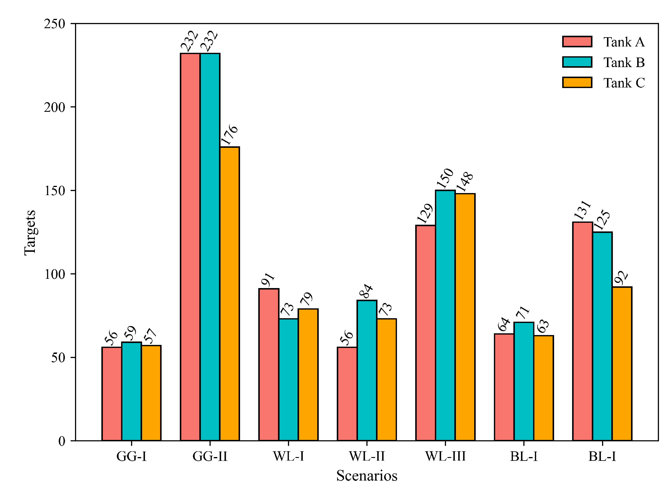
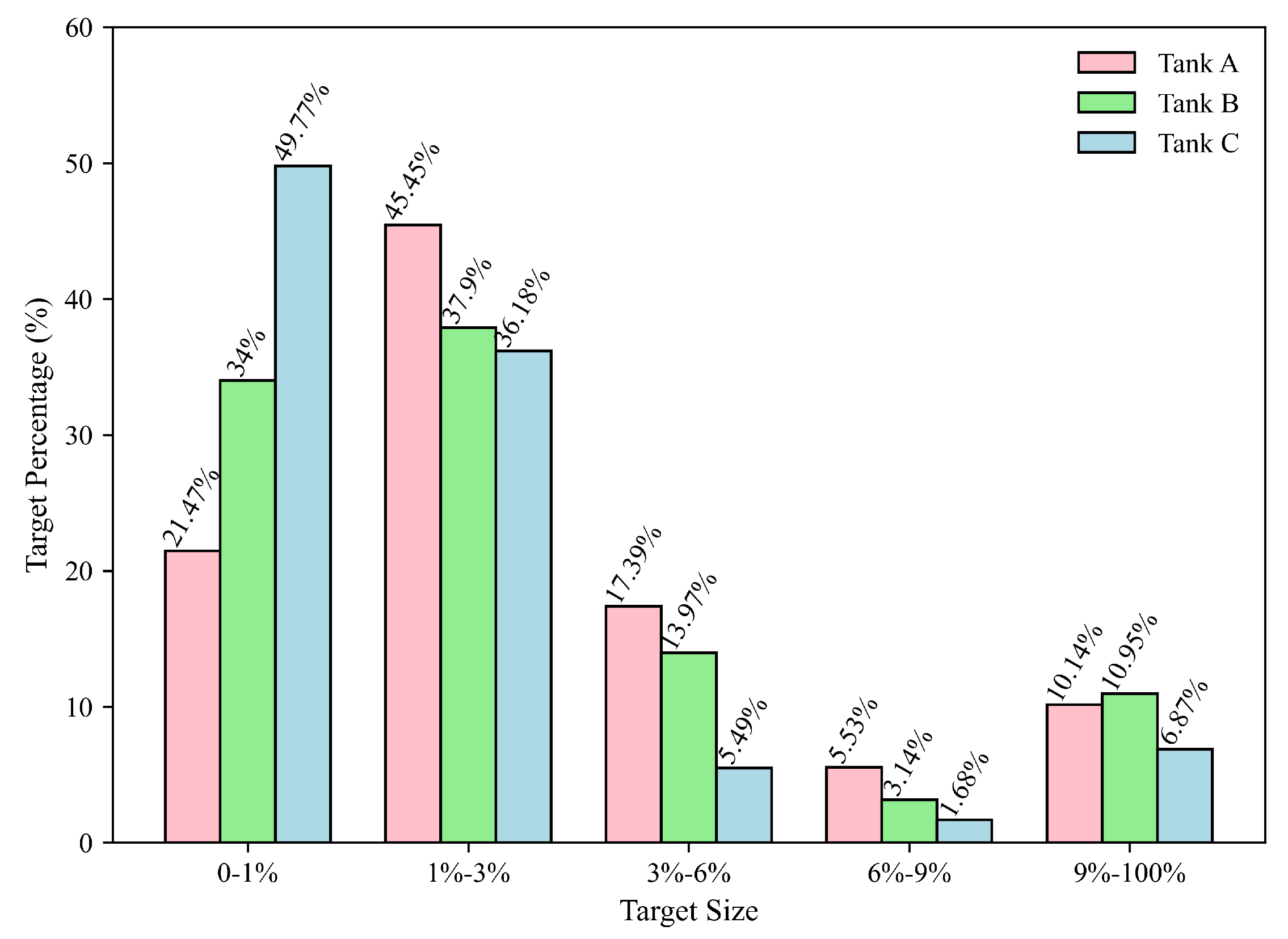
2.2. Dataset Statistics

The UAVT-3 database includes 1263 images with a resolution of $1024\times 768$, 7 scenes, 3 types of tanks, and 2241 marked objects. The number of tanks of each type in the seven scenes is shown in Figure 2. It can be seen that the number of tanks of the three types in each scene is relatively close, and the numbers of Tank A, Tank B, and Tank C are 759, 794, and 688, respectively, which are also very close.

Figure 3 shows the distribution of object sizes, where the x-axis denotes the normalized object size, i.e., the area ratio of the object to its image, and the y-axis represents the ratio of the objects to the total tanks in the same class. It can be seen that the target size is mostly concentrated in the 0–1% and 1–3% regions, and the proportion of the three class tanks in the two regions are 66.85%, 71.9%, and 85.95%, respectively. According to [11], most of the objects in the UAVT-3 database are small objects; therefore, detecting objects in the UAVT-3 dataset can be regarded as a small object visual recognition task.

3. UAVT-YOLOv5 Model

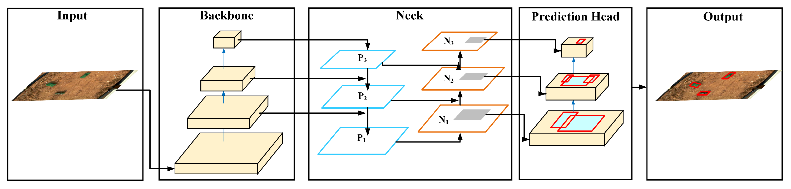
3.1. Structure of UAVT-YOLOv5

YOLOv5 is a regional regression-based one-stage object detection model, which models object detection as a regression problem and predicts the object location by regression. It predicts the object bounding box and category by regression, which only looks at the image one time with a single network. The basic idea of YOLOv5 is to divide the image into $S\times S$ grids, and the cell that the object center is located in is responsible for detection. It takes three scales of the feature map to make a multi-scale prediction. The image is divided into a different number of cells according to the feature map scale, and three bounding boxes will be predicted for each cell. The bounding box is expressed as (x, y, w, h, c), where (x, y) represents the coordinate of the object center relative to the left upper corner of the cell to which the object belongs, (w, h) represents the ratio of the object width and height to the image, and c indicates the confidence of the bounding box containing an object. Meanwhile, the class probabilities of the object are also predicted for each bounding box. Therefore, there are $3\times (5+m)$ values that need to be regressed by the model for each cell, where m is the total number of classes for detection.

Figure 4 shows the flowchart of the proposed UAVT-YOLOv5 being kept the same as that of YOLOv5, which consists of input, including data augmentation, backbone, neck, prediction head, and output, including post-processing. In the input, several data augmentation techniques have been used in the original model, such as mosaic, copy-paste, mix-up, and so on. The backbone is designed to extract visual features, which incorporated the Cross Stage Partial (CSP) [12] block and the Spatial Pyramid Pooling Fast (SPPF) [10] block into the DarkNet53. The neck takes the Feature Pyramid Network (FPN) [13] and Path Aggregation Network (PAN) [14] to realize the information sharing from both bottom-up and up-bottom. The head is to regress the bounding box and class probabilities. In the post-processing of the output, the bounding box with a confidence lower than the threshold will be removed, and Non-Maximum Suppression (NMS) is then used to filter the remaining bounding boxes to obtain the final predicting box. In order to detect object detection of UAV reconnaissance image, the proposed UAVT-YOLOv5 was improved from YOLOv5 as follows.

1.

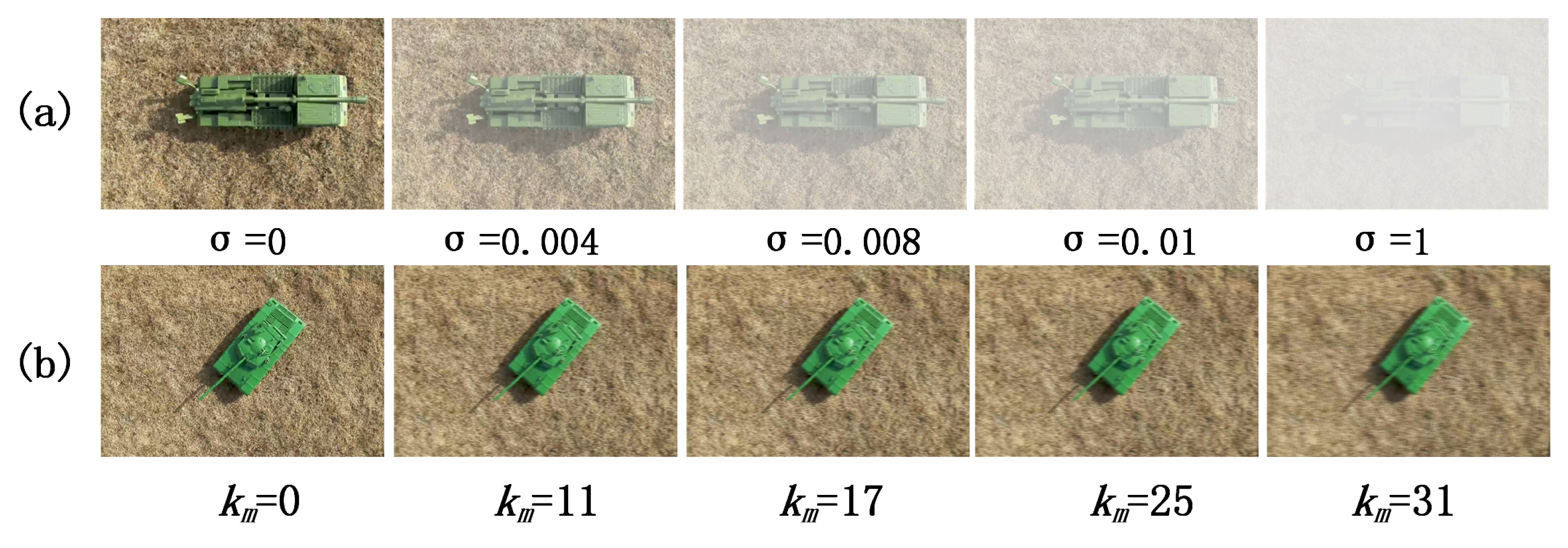
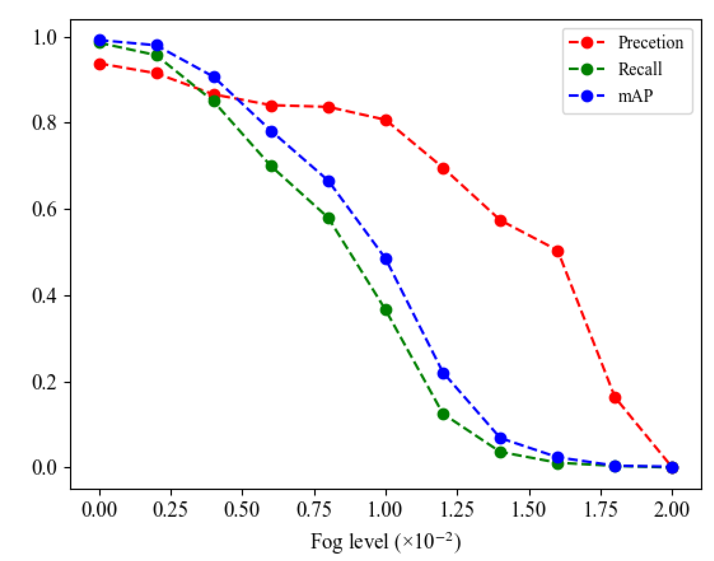
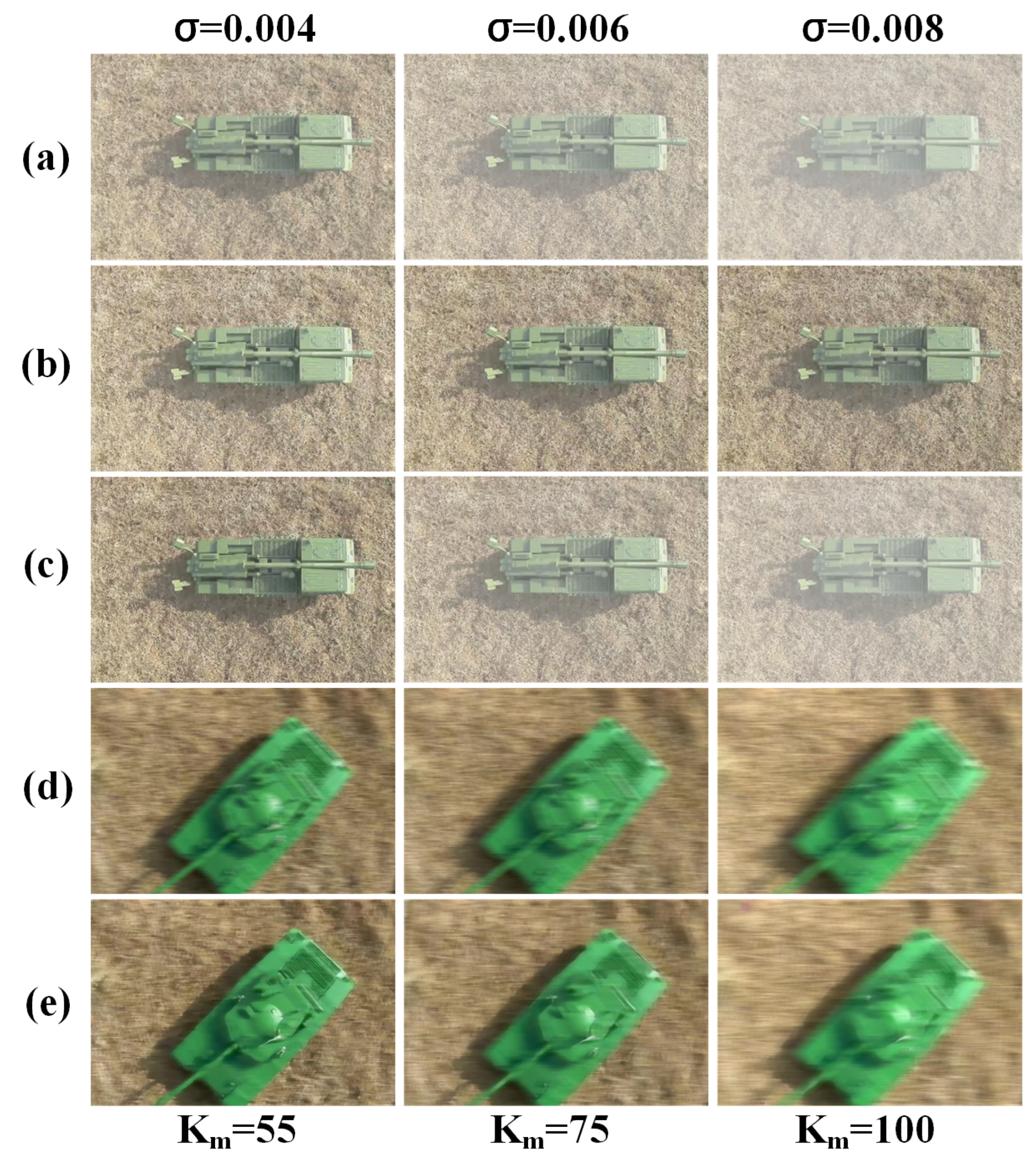
In the input part, data augmentation of blurred images is adopted to improve the accuracy of fog blur and motion blur images, which will be detailed in Section 3.2.

2.

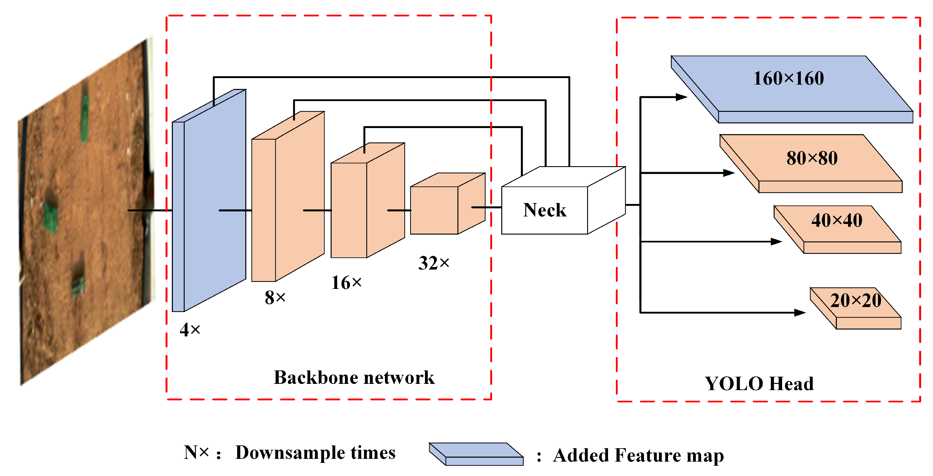
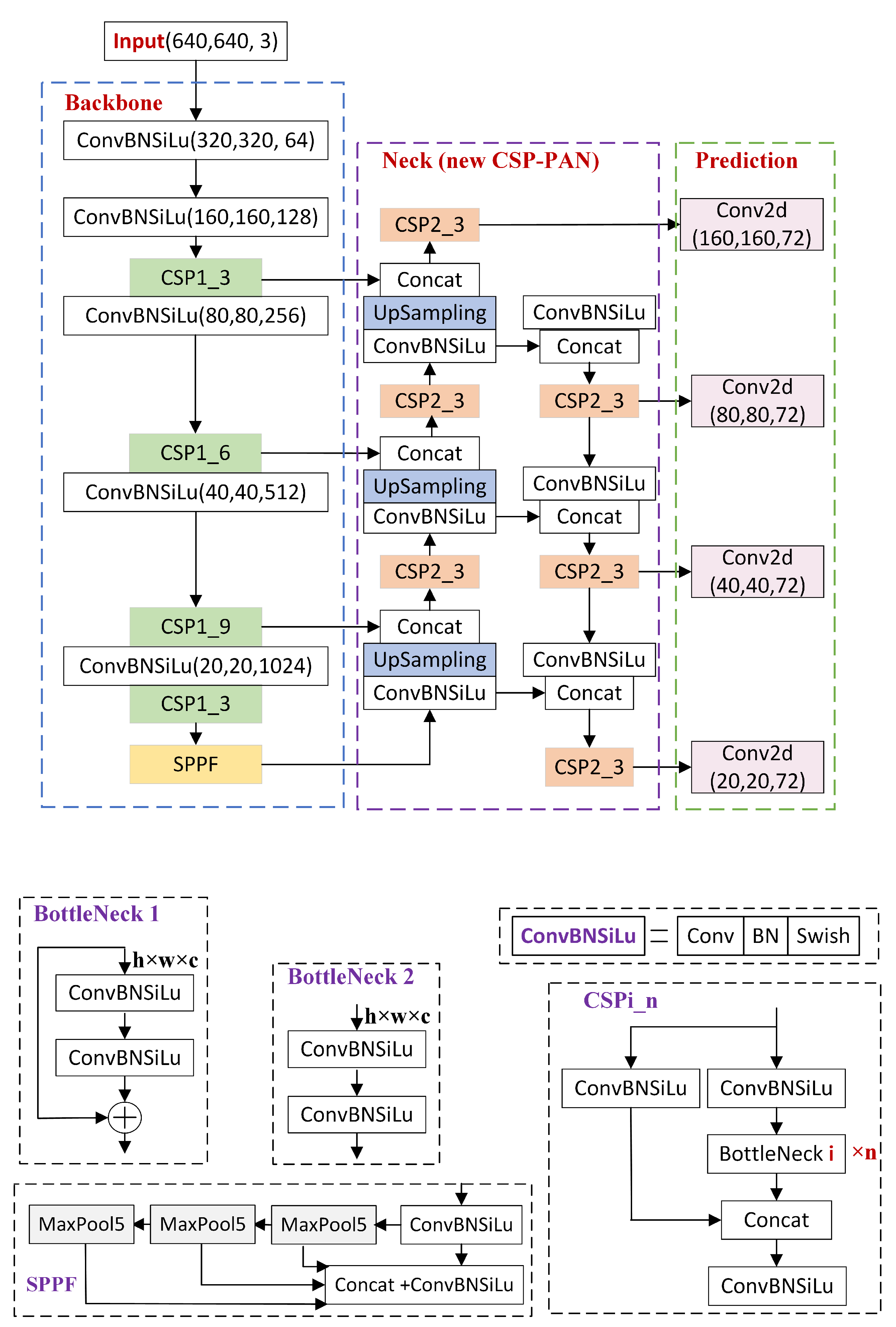
In the neck part, to improve the recognition ability of small objects, a larger scale feature map is added to mine more features from the small target, and the multi-scale feedback mechanism is introduced to combine the global context information, which will be detailed in Section 3.3.

3.

The box confidence loss function and anchor priors are optimized by increasing the penalty of small objects and by re-clustering the object boxes of UAVT-3 with a k-means algorithm, which will be Section 3.4 and Section 3.5, respectively.

3.2. Data Augmentation of Blur Image

The UAV images were usually captured outdoors, which were easily affected by dust and mist in the atmosphere and introduced fog blur. Moreover, UAVs are susceptible to the influence of airflow to produce jitter, which will introduce motion blur. Figure 5a,b show the UAV images with fog blur and motion blur, respectively. $\sigma$, $K_m$ denotes the blur factors of fog blur and the motion blur, larger $\sigma$ and $K_m$ mean greater distortion. It can be seen that both the fog blur and motion blur reduced the image quality and contrast, which may reduce the detection accuracy.

Figure 6 shows the prediction accuracy of the fog-blurred images. We can see that the model is sensitive to fog blur distortion, the recall, prediction, and mAP values dropped rapidly with the increase in fog blur distortion. Several data augmentation techniques have been used in YOLOv5, such as rotation, color transformation, mosaic, and copy-paste. However, the fog and motion blur samples were not used in training, and it resulted in the poor performance of the model in detecting fog and motion blur images. Fog and motion blur are the two most common distortions in UAV images. Therefore, we introduced fog- and motion-distorted images in training to improve the detection accuracy of fog and motion-blur images. The details will be illustrated in Section 4.4.

3.3. Feature Extractor and Fusion

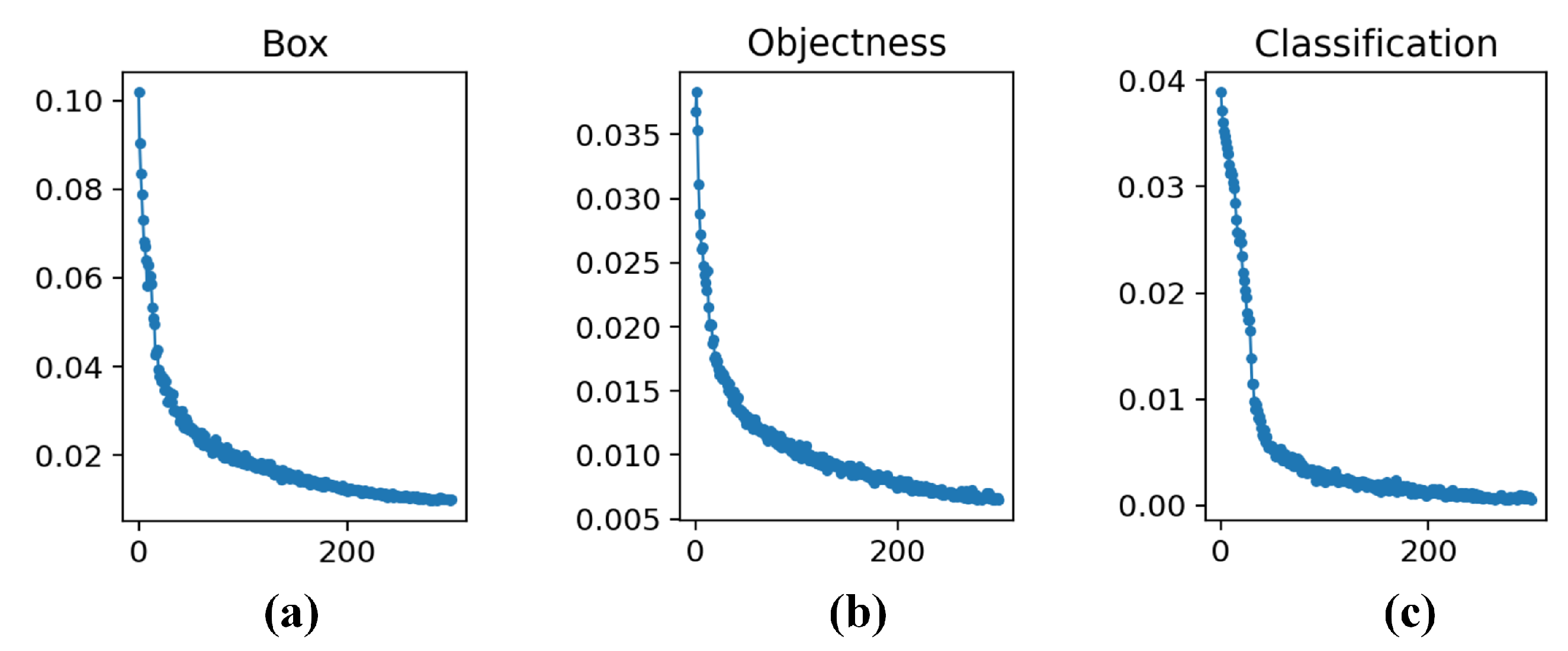
The original YOLOv5 used three scale feature maps ($52\times 52$, $26\times 26$, $13\times 13$) to detect objects of different sizes; the backbone network downsampled the input image by $8\times$, $16\times$, and $32\times$ to obtain the corresponding feature maps feed into the feature fusion network. According to the Feature Pyramid Network (FPN), the small-size feature map is not effective for detecting small objects since the location information is lost after a series of convolutions. The large-size feature map obtained after shallow convolution retains accurate object location information, which is more suitable for small object detection. The UAV images were usually captured at high altitudes, in which the objects are relatively small. As shown in Figure 7, a larger feature map with $160\times 160$ was added to this work, which was obtained through $4\times$ downsampling of the input ($640\times 640$) by the backbone network. The new feature map was obtained through fewer convolutions and had a smaller receptive field; it preserves more location information and can improve the accuracy in small object detection.

The feature map obtained after different convolutional layers contains different feature information. Generally, the feature map obtained by shallow convolutions has a higher resolution and richer location information, but contains low-level semantic feature information. It is more powerful for small object detection but not suitable for complicated object recognition. The feature map obtained after deep convolutions has high-level semantic information but lost more location information, which is powerful in complicated object recognition but not suitable for small objects. Therefore, it is necessary to fuse the low-level and high-level feature maps in UAV object detection. It incorporated Feature Pyramid Network (FPN) and Path Aggregation Network (PAN) to perform feature fusion. The FPN transmits high-level semantic features from top to bottom, which aims to improve complicated object recognition for large-scale feature maps. The PAN transmits the location information from the bottom up, which aims to improve the location ability for small-scale feature maps. In this work, the added feature map incorporated the CSP FPN-PAN structure, and the modified network structure is shown in Figure 8.

3.4. Loss Function

In YOLOv5, the loss function shown in Equation (2) consists of the classification loss $L_{cls}$, location loss $L_{loc}$, and object confidence loss $L_{obj}$, which measure the distance between the anchor box classification and the ground-truth class, the predicting box and labeled box, and the possibility of the anchor box being an object, respectively.

$$Loss={\lambda }_1{L}_{cls}+{\lambda }_2{L}_{loc}+{\lambda }_3{L}_{obj}.$$

(2)

Both $L_{cls}$ and $L_{obj}$ used binary cross-entropy loss, $L_{cls}$ only computes the loss of positive samples, while $L_{obj}$ computes the loss of all positive and negative samples. $L_{obj}$ used CIoU loss computing for the loss of positive samples. ${\lambda }_1$, ${\lambda }_2$, and ${\lambda }_3$ are the weighting factors, which were set as that in YOLOv5 in this work. The object confidence loss $L_{obj}$ was obtained as

$$L_{obj}={\beta }_1{L}_{obj}^s+{\beta }_2{L}_{obj}^m+{\beta }_3{L}_{obj}^l.$$

(3)

where $L_{obj}^s$, $L_{obj}^m$, and $L_{obj}^l$ denote the loss of small, medium, and large-scale feature maps, where ${\beta }_1$, ${\beta }_2$, and ${\beta }_3$ are the weighting factors, which were set as 4.0, 1.0, and 0.4, optimized in COCO dataset [15]. In this work, we add a new loss item ${\beta }_4{L}_{obj}^n$ to Equation (3) for the newly added feature map, and ${\beta }_1$, ${\beta }_2$, and ${\beta }_3$, and ${\beta }_4$ are set based on the UAVT-3 database. The four factors were first set as 4.0, 1.0, 0.4, and 0.2 by borrowing the idea in YOLOv5 that as a small object is difficult to detect, it should be given a larger weighting in the loss. Moreover, we also take the training sample distribution into consideration due to that the class with fewer samples is more difficult to recognize. The final weights were obtained by ${\beta }_i\times r_i$, where $r_i$ was the ratio factor obtained by following

$$r_i=norm(1/R_i),$$

(4)

where $R_i$ denotes the sample ratio of $i_{th}$ scale in k-means clustering, and $norm\left(\right)$ denotes the normalization function.

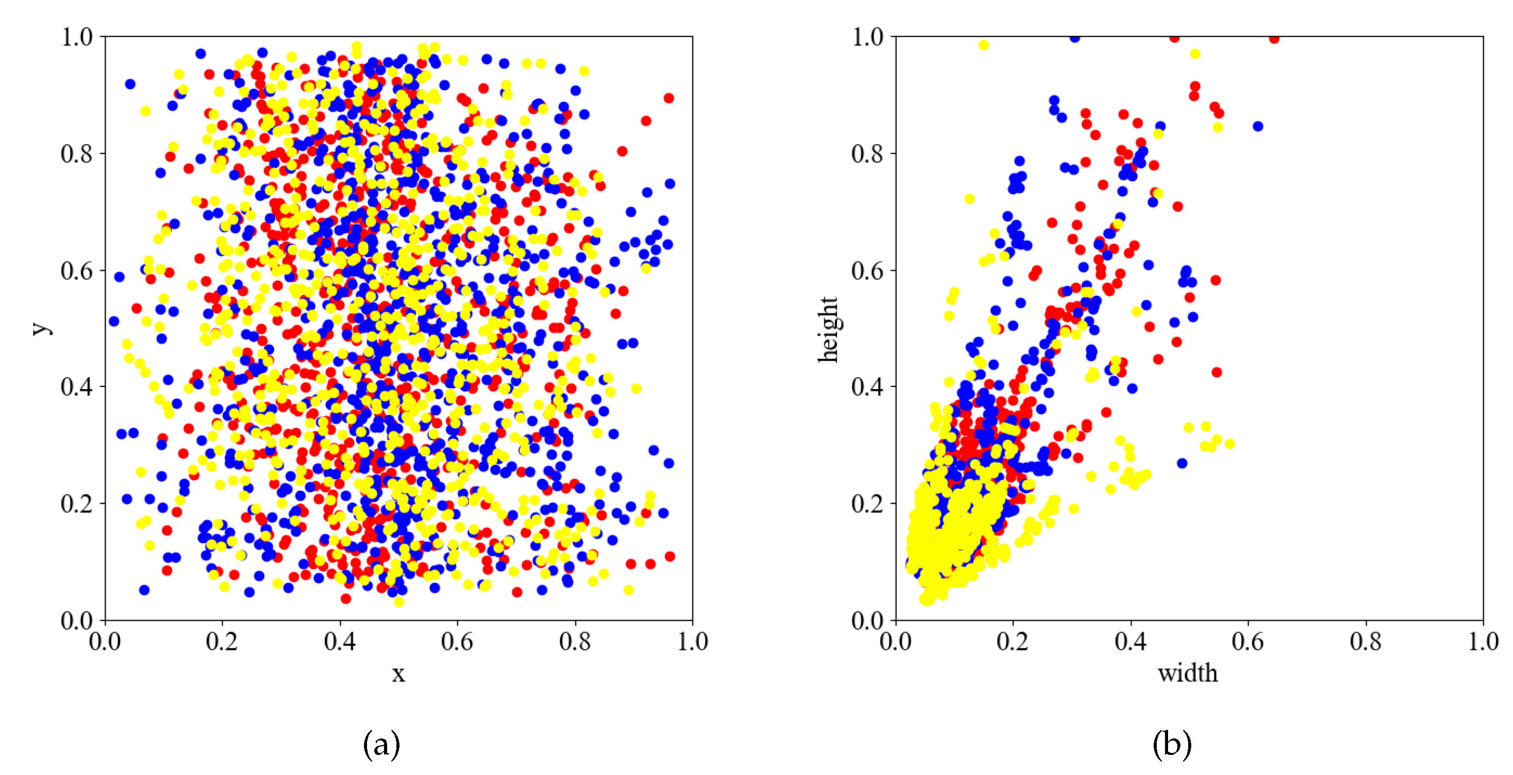
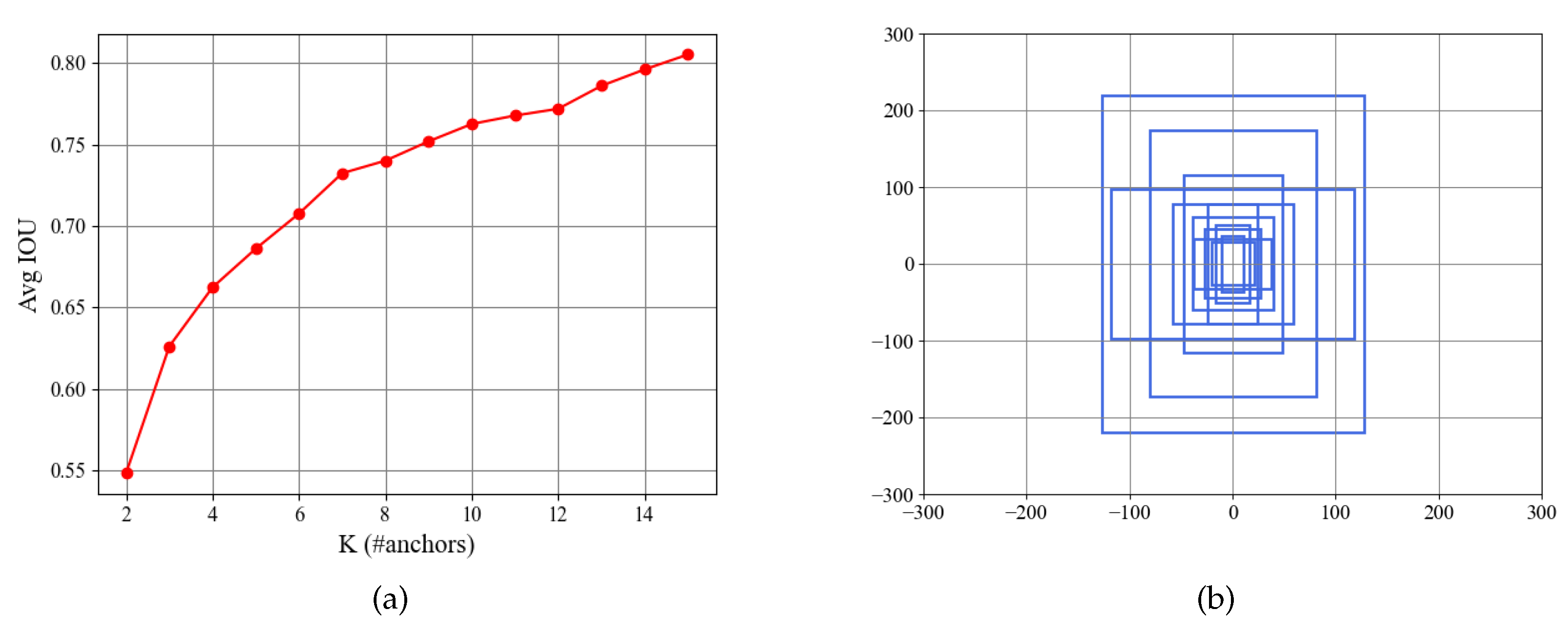
3.5. Anchor Box Setting

Figure 9 shows the distribution of the object bounding boxes of the UAVT-3 dataset, where the center location, width, and height are normalized with the image size. From Figure 9a, it can be seen that the center location points are nearly spread all over the figure, which means that the tanks appear in different locations. From Figure 9b, we can see that most points are located in the left corner, which means that the objects of the UAVT-3 dataset are small objects.

The anchor boxes were obtained by using K-means to cluster ground truth boxes of the COCO dataset [15], which is not the optimal choice for UAVT-3 since there are some differences between COCO and UAVT-3. Therefore, it is necessary to re-cluster to obtain anchor boxes suitable for the UAVT-3 dataset. The Euclidean distance is one of the most popular similarity metrics in K-means clustering. However, it is very sensitive to the size of the target box. The following distance function was designed using Intersection over Union (IoU)

$$d(B_i,C)=1-IoU(B_i,C),$$

(5)

where $B_i$ denotes the $i_{th}$ box, and C denotes its corresponding center point in the clustering. Figure 10a shows the clustering results, where the x-axis represents the number of clustering center points, and the y-axis represents the average IoU. It can be seen that when K is over 12, the average IoU rises slowly. Therefore, 12 can be seen as the inflection point, which was selected as the number of anchor boxes shown in Figure 10b. As shown in

Table 1. The size of anchor boxes for the four feature maps.

Feature Map	Size of Anchor Box
160 × 160	(22, 74)	(32, 102)	(41, 55)
80 × 80	(48, 156)	(54, 89)	(76, 64)
40 × 40	(79, 121)	(95, 230)	(117, 156)
20 × 20	(161, 347)	(236, 195)	(255, 440)

, three boxes were selected for each feature map.

4. Experimental Results and Analysis

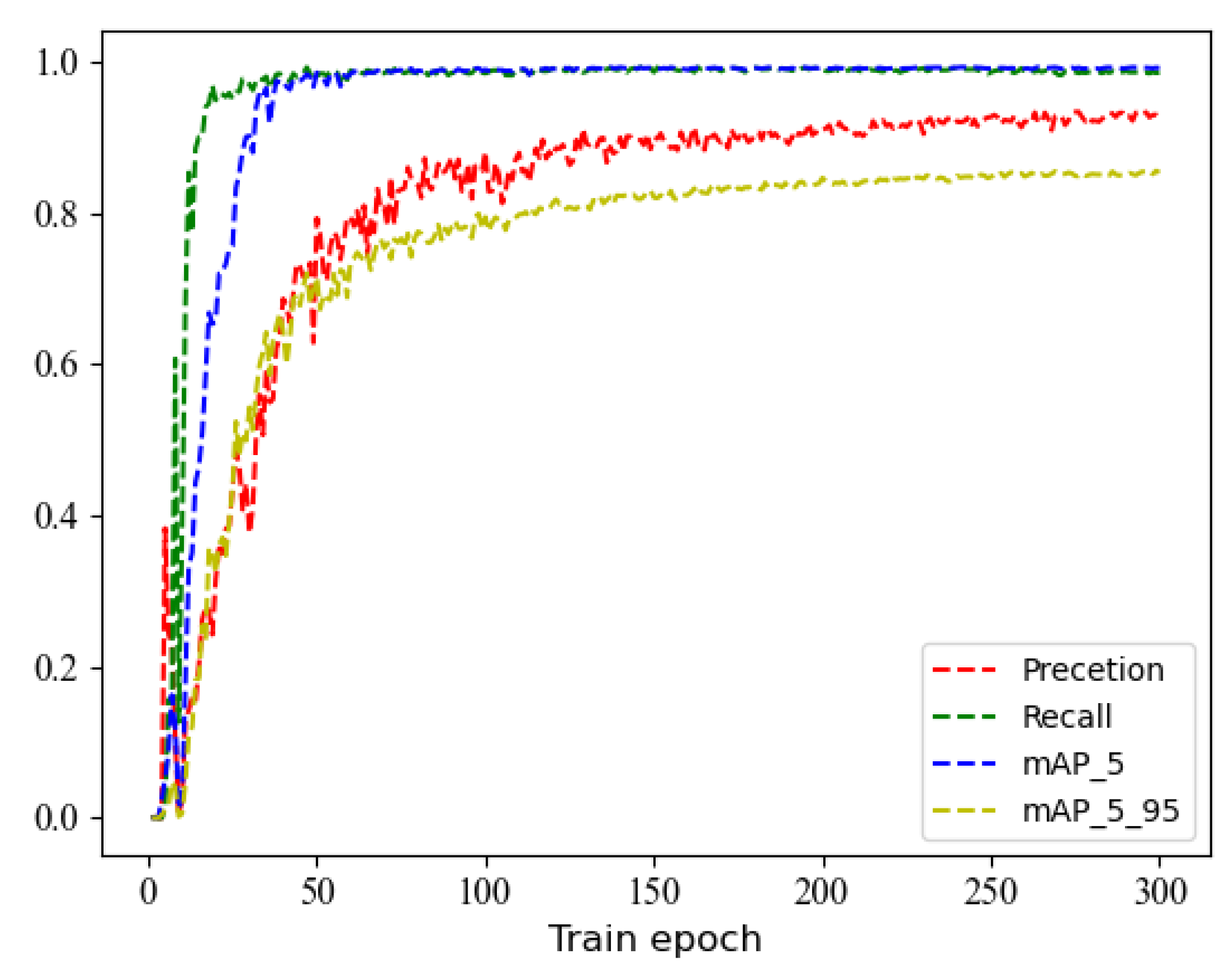
4.1. Experimental Setting and Model Training

The experiments were performed on a graphics workstation equipped with an Intel Core I9-10900X CPU, 64GB of RAM, and an Nvidia GeForce RTX 3080 Ti GPU with 12 GB memory. All three types of tanks in each scene were divided into training samples and test samples according to the ratio 2:1. The training samples and test samples of all scenes constituted a training set and test set. After the split, the samples of the training set and test set are 842 and 421, respectively. All of the test models were fine-tuned on the UAVT-3 dataset based on the weights provided in the original papers.

In this work, Average Precision ($AP$), Mean Average Precision ($mAP$), and Frames per Second ($FPS$) were adopted as the evaluating metrics, which also have been widely used in object detection. $AP$ refers to the area of the Precision (P)-Recall (R) curve, which can be obtained by Equation (6)

$$AP={\int }_0^{1}PdR.$$

(6)

$mAP$ refers to the mean AP of all detection classes, which can be obtained by Equation (7)

$$mAP=\frac{1}{N}\sum _{i=1}^{N}A{P}_i,$$

(7)

in which N denotes the detecting classes, and N is 3 in this work. For both $AP$ and $mAP$, a larger value means better performance. P and R in Equations (6) and (7) can be obtained by Equations (8) and (9), respectively,

$$P=\frac{TP}{TP+FP}=\frac{TP}{alldections},$$

(8)

$$P=\frac{TP}{TP+FN}=\frac{TP}{allgroundtruths},$$

(9)

where True Positives ($TP$), False Positives ($FP$), and False Negatives ($FN$) denote the number of correct detection boxes, false detection boxes, and missed detection boxes, respectively.

In order to train the proposed model, we first pre-trained the model on the COCO dataset [15] for parameter initialization and then fine-tuned the model on UAVT-3. The training iterations of fine-tuning were set to 299, in which the best model was selected as the final model. Figure 11 and Figure 12 show the training loss and detection accuracy in fine-tuning. Figure 11a–c show the training loss of the box regression, confidence, and classification. It can be seen from Figure 11 that all three types of losses decreased sharply with the iteration increase before 50 epochs, then changed slowly, and finally, transitioned to smooth. Figure 12 shows the changes in P, R, mAP-5, and mAP-5-95 during training, from which it can be seen that the four metrics rise sharply at the beginning, rise slowly after 50 epochs of training, and then become stable. It can be seen that the training loss and detection accuracy become stable after 200 epochs, which can demonstrate that the model was convergent.

4.2. Performance of Different Detection Models

In order to make a pair performance comparison, all of the compared models, including Faster-RCNN [4], SSD [6], YOLOv1 [5], YOLOv2 [7], YOLOv3 [8], YOLOv4 [9], and YOLOv5, were first trained on the COCO dataset [15] and fine-tuned on UAVT-3. The experimental results are shown in

Table 2. Performance of the compared detection models. The bold part denotes the best performance.

Models	AP (%)			mAP (%)	F1-Score (%)	Times (s)	FPS
	Tank A	Tank B	Tank C
Faster-RCNN [4]	84.05	72.22	64.85	73.70	74.40	0.319	3.14
SSD [6]	96.01	97.14	95.33	96.16	91.98	0.0245	40.8
YOLOv1 [5]	71.21	57.60	60.23	63.02	61.20	0.069	14.4
YOLOv2 [7]	80.40	72.50	79.64	77.52	76.35	0.050	20.1
YOLOv3 [8]	98.00	91.67	98.00	95.22	82.22	0.041	24.76
YOLOv4 [9]	96.75	95.20	97.33	96.42	95.05	0.046	21.3
YOLOv5	97.10	97.28	97.40	97.16	96.16	0.020	50
Proposed	99.20	99.00	99.40	99.20	98.31	0.025	40

, from which we can see that the mAP and F1-score (mAP, F1-score) of YOLOv1, Faster-RCNN, and YOLOv3 are (63.02%, 61.20%), (73.70%, 74.40%), (77.52%, 76.35%), which are lower than those of the other models. The (mAP, F1-score) of YOLOv3, YOLOv4, and YOLOv5 is (95.22%, 82.22%), (96.42%, 95.05%), and (97.36%, 96.16%), respectively, all of which are higher than that of SSD (94.16%, 91.98%), and YOLOv5 reaches the highest (mAP, F1-score) (97.36%, 97.16%) among the comparison models. The (mAP, F1-score) of the proposed model reaches (99.20%, 98.31%), which has the best performance. The proposed model yields an increase of (1.84%, 2.15%) compared with the original YOLOv5 in (mAP, F1-score), of which the AP of the three tanks exceeded 99%. The improvements in the model in mAP and AP are due to the modifications on YOLOv5. In the computation complexity, YOLOv5 has the best performance since it has the lowest time per image (0.020 s) and the largest FPS 50. The proposed model needs 0.025 s per image, and its FPS is 40, which has a slightly higher time complexity. However, it is enough for real-time detection.

4.3. Analysis of Feature Visualization

The deep CNN-based model is poor in explanation due to its black box working manner, and lots of work about feature visualization have been proposed to improve the interpretability of deep models. Class Activation Mapping (CAM) [16,17,18,19,20], i.e., heat map or salience map, is one of the most popular feature visualization techniques. The generated CAM map shows the importance of regions in the decision of deep models, of which the larger value means more contributions. The CAM methods can be roughly divided into the gradient-free method [16,17,18] and the gradient-based method [19,20]. In this work, we took Grad-CAM [19] to generate CAM maps for exploring the mechanism of the proposed model, and examples of CAM maps are shown in Figure 13. It can be seen that the discriminant region is the turret; the difference in the turret among the three types of the tank is salient. Therefore, it can be seen as reasonable that the proposed model identifies tanks based on the turret, since it is similar to human beings. In addition, the discriminant region is very stable and was not affected by the changes in scene and object size. It can demonstrate that the model learned the distinguishing characteristics of objects, and the model is robust. The objects in the second, third, and fourth columns are smaller than that in the first column; we can see that the discriminant region in the second, third, and fourth columns are larger than that in the first column. As we know, the smaller object is more challenging to detect. Therefore, the model needs more information, and the discriminant region becomes larger to include more features. We can also see that the background of the fifth column is more complex than that of the first column, and the distinguishing area also becomes larger. Since the object located in the complicated background is also more challenging, the model also needs more information in the decision. It can be concluded that the model recognizes tanks by the turret, which needs more information on tanks with a small size and in a complicated background.

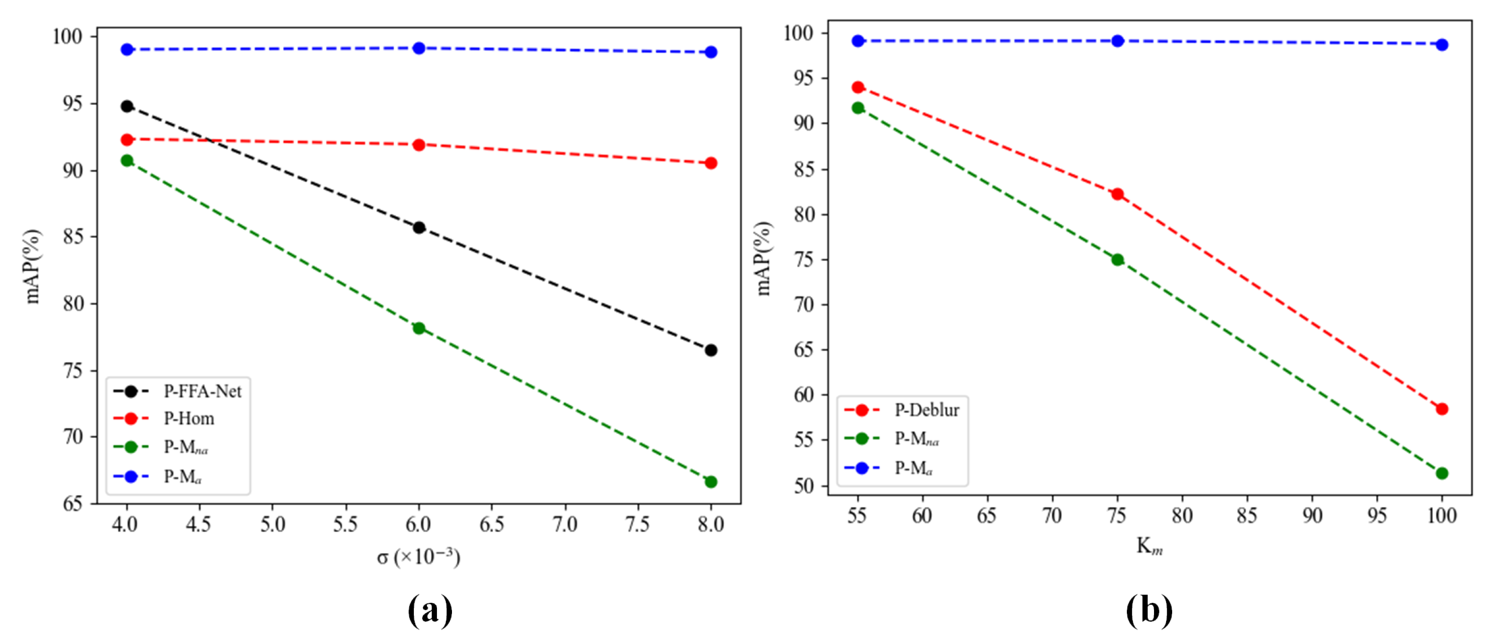
4.4. Effects of the Data Augmentation

In this section, we evaluate the data augmentation of blurred images. Let $M_{na}$ denote the model trained on the UAVT-3 training set, $M_a$ denote the model fine-tuned using blurred images with distortion $D_j^i$ from $M_{na}$, where i denotes the blur type (fog blur and motion blur), j denotes the distortion degree, and three distortion degrees were selected in this work. There are 12 $M_a$ models evaluated on the corresponding test set, i.e., i and j were kept the same in training and testing. The experiment’s results are shown in

Table 3. Evaluation Results on Fog and Motion Blur Images.

Blur Type	Blur Degree	Models	P (%)	R (%)	mAP (%)
Fog	$\sigma$ = 0.004	$M_{na}$	86.6	85.0	90.7
		$M_a$	92.8	98.6	99.0
	$\sigma$ = 0.006	$M_{na}$	84.1	70.0	78.2
		$M_a$	93.8	98.6	99.1
	$\sigma$ = 0.008	$M_{na}$	83.7	58.0	66.7
		$M_a$	98.2	99.2	98.8
Motion	$K_m$ = 55	$M_{na}$	91.5	87.4	91.8
		$M_a$	91.6	98.9	99.1
	$K_m$ = 75	$M_{na}$	80.0	69.5	75.0
		$M_a$	90.8	99.1	99.1
	$K_m$ = 100	$M_{na}$	69.5	42.9	51.3
		$M_a$	93.9	98.2	98.8

. $\sigma$ and $K_m$ denote the blur factors of fog blur and motion blur; larger $\sigma$ and $K_m$ means greater distortion. For the fog blur, it can be seen that when $\sigma$ was set as 0.004, 0.006, and 0.008, the (P, R, mAP) of model $M_{na}$ are (86.6%, 85.0%, 90.7%), (84.1%, 70.0%, 78.2%), (83.7%, 58%, 66.7%), while those of model $M_a$ is (92.8%, 98.6%, 99.0%), (93.8%, 98.6%, 99.1%), (98.2%, 99.2%, 98.8%). The (P, R, mAP) increased (6.2%, 13.6%, 8.3%), (9.7%, 28.6%, 20.9%), (14.5%, 41.2%, 31.2%), and the average increase is (13.4%, 27.8%, 20.1%). It can be concluded that the P, R, and mAP of model $M_{na}$ reduced greatly with the increase in $\sigma$. However, the accuracy of model $M_a$ improved greatly after fine-tuning using the data augmentation of blur images. The same conclusion can also be obtained from the motion blur part. The P, R, and mAP values of $M_{na}$ decrease significantly with the increase in $K_m$, and the accuracy of model $M_a$ improved greatly after fine-tuning the motion-blurred images. The average improvement of (P, R, mAP) is (11.8%, 32.1%, 26.3%) when $K_m$ was set as 55, 75, and 100. Therefore, it can be concluded that data augmentation of blur images can greatly improve the accuracy of the blurred images, i.e., improve the generalization ability in practice.

4.5. Further Discussion

The UAV images were usually degraded by fog blur and motion blur, which not only affect the visual quality but also affect the accuracy of deep models since the existing deep models were usually trained on high-quality samples. Training deep models on degraded samples is an effective way to improve the performance. However, degraded images are difficult to collect. Enhancing the image quality by a pre-processing method is another effective way to improve the image quality and performance of deep models. We test homomorphic filter [21] and FFA-Net [22] to pre-process the fog-blurred images and DeblurGAN [23] to pre-process the motion-blurred images. Figure 14 shows the pre-processed results, where (a) and (d) are the fog-blurred and motion-blurred images, (b) and (c) are the pre-processed images by homomorphic filter and FFA-Net, respectively, and (e) is the de-blurred images by DeblurGAN. It can be seen that the visual quality of the fog-blurred and motion-blurred images was improved obviously. Then, we evaluated the proposed UAVT-YOLOv5 trained on the free-blurred training set on the pre-processed images from the blurred test images of UAVT-3. Figure 15a,b show the results of fog-blurred and motion-blurred images, P-Hom and P-FFA-Net denote homomorphic filter and FFA-Net pre-processing in Figure 15a, P-Deblur denotes DeblurGAN pre-processing in Figure 15b, P-Ma and P-Mna denote data augmentation of fog blur without any pre-processing and data augmentation in Figure 15a and in Figure 15b. It can be seen that the mAP of P-Hom and P-FFA-Net is higher than that of P-Mna, which means the pre-processing by the homomorphic filter and P-FFA-Net improved the performance. However, the mAP of P-Hom and P-FFA-Net is still lower than that of P-Ma, especially when the image has a heavy degradation. The same phenomenon can be seen from the motion blur shown in Figure 15a. It can be concluded that the accuracy from pre-processing was improved and deserves further study on pre-processing methods aiming for performance improvement.

In splitting the UAVT-3 database into training and test sets, Scene-based Splitting (SS) and Random Splitting (RS) schemes were tested. In SS schemes, the samples of five scenes were selected as the training set and the rest as the test. Two SS schemes were tested, the training and test scenes of the SS1 scheme are (GG-I, WL-I, WL-II, WL-III, Bush-I) and (Bush-I, GG-II). In the SS2 scheme, the training and test set are (GG-I, WL-I, WL-II, Bush-I, GG-II) and (WL-III, Bush-I). In the RS scheme, all of the samples in UAVT-3 were divided into training and test sets in a random way at a ratio of 2:1. The experimental results are shown in

Table 4. Performance on different splitting schemes. The bold part denotes the best performance.

Schemes	AP (%)			mAP (%)
	Tank A	Tank B	Tank C
SS1	14.60	19.40	45.20	26.40
SS2	49.80	59.00	86.20	65.00
RS	57.20	85.70	93.00	78.63

. It can be seen that the mAP of SS1 and SS2 are 26.5% and 65%, respectively, which are very slow. Moreover, the mAP gap between SS1 and SS2 is very large. It can be said that the accuracy is related to the division of the scenes. The mAP value of the RS scheme is 78.6%, which is higher than that of SS1 and SS2; the reason is that the model has been seen all over the scenes. It can be concluded: (1) In SS schemes, the accuracy of the model was very low and also affected by the scene division. (2) The model trained on the samples across all the scenes has relatively high accuracy. We divided the tanks into training and test sets at a ratio of 2:1 across three types of tanks in each scene. Therefore, the model can be trained on all scenes, and the samples for each class can remain in relative balance.

5. Conclusions

In this work, we simulated Unmanned Aerial Vehicle (UAV) low-altitude reconnaissance and constructed the UAV reconnaissance image tank dataset UAVT-3. Then, we proposed UAVT-YOLOv5 from YOLOv5 by using blurred images as data augmentation, adding a large-scale feature map, optimizing the loss function, and clustering anchor boxes. The feature visualization technique Class Action Mapping (CAM) was also introduced to explore the mechanism of the proposed model. The experimental results show that mAP reaches 99.2%, an increase of 2.1% compared to YOLOv5, and the detection speed is 40 frames per second. Moreover, it is found that mAP decreases sharply when detecting fog and motion blur images. However, the fine-tuned model using the blurred images as training can improve mAP by 20.4% and 26.6% for fog and motion blur images, respectively. The CAM maps show that the discriminant region of tanks is the turret for UAVT-YOLOv5.

References

1. Krizhevsky, A.; Sutskever, I.; Hinton, G. ImageNet classification with deep convolutional neural networks. Commun. ACM 2017, 60, 84–90. [Google Scholar] [CrossRef] [Green Version]
2. Girshick, R.; Donahue, J.; Darrell, T.; Malik, J. Rich feature hierarchies for accurate object detection and semantic segmentation. In Proceedings of the IEEE Conference on Computer Vision and Pattern Recognition, Columbus, OH, USA, 23–28 June 2014; Volume 10, pp. 580–587. [Google Scholar]
3. Girshick, R. Fast R-CNN. In Proceedings of the IEEE International Conference on Computer Vision, Santiago, Chile, 11–18 December 2015; Volume 10, pp. 1440–1448. [Google Scholar]
4. Ren, S.; H, K.; Girshick, R. Faster R-CNN: Towards real-time object detection with region proposal networks. IEEE TPMI 2016, 39, 1137–1149. [Google Scholar] [CrossRef] [PubMed] [Green Version]
5. Redmon, J.; Divvala, S.; Darrell, T.; Girshick, R.; Farhadi, A. You only look once: Unified, real-time object detection. In Proceedings of the IEEE Conference on Computer Vision and Pattern Recognition, Las Vegas, NV, USA, 27–30 June 2016; pp. 779–788. [Google Scholar]
6. Liu, W.; Anguelov, D.; Erhan, D.; Szegedy, C.; Reed, S.; Fu, C.Y.; Berg, A.C. SSD: Single Shot MultiBox Detector. In Proceedings of the 14th European Conference, Amsterdam, The Netherlands, 11–14 October 2016; Springer: Cham, Switzerland, 2016; pp. 21–37. [Google Scholar]
7. Redmon, J.; Farhadi, A. YOLO9000: Better, faster, stronger. In Proceedings of the IEEE Conference on Computer Vision and Pattern Recognition, Honolulu, HI, USA, 21–26 July 2017; pp. 7263–7271. [Google Scholar]
8. Redmon, J.; Farhadi, A. Yolov3: An incremental improvement. arXiv 2021, arXiv:1804.02767. [Google Scholar]
9. Bochkovskiy, A.; Wang, C.; Yuan, H.; Liao, M. YOLOv4: Optimal Speed and Accuracy of Object Detection. arXiv 2021, arXiv:2004.10934. [Google Scholar]
10. He, K.; Zhang, X.; Ren, S.; Sun, J. Spatial pyramid pooling in deep convolutional networks for visual recognition. IEEE Trans. Pattern Anal. Mach. Intell. 2014, 37, 1904–1916. [Google Scholar] [CrossRef] [PubMed]
11. Zhu, Z.; Liang, D.; Zhang, S.; Huang, X.; Li, B.; Hu, S. Traffic-sign detection and classification in the wild. In Proceedings of the IEEE Conference on Computer Vision and Pattern Recognition, Las Vegas, NV, USA, 27–30 June 2016; Volume 10, pp. 2110–2118. [Google Scholar]
12. Wang, C.; Liao, H.; Wu, Y.; Chen, P.; Hsieh, J.; Yeh, I. CSPNet: A new backbone that can enhance learning capability of cnn. In Proceedings of the CVPR Workshop, Seattle, WA, USA, 14–19 June 2020; pp. 1571–1580. [Google Scholar]
13. Lin, T.; Dollar, P.; Girshich, R.; He, K.; Hariharan, B.; Belongie, S. Feature pyramid networks for object detection. In Proceedings of the IEEE Conference on Computer Vision and Pattern Recognition, Honolulu, HI, USA, 21–26 July 2017; pp. 936–944. [Google Scholar]
14. Li, H.; Xiong, P.; An, J.; Wang, L. Pyramid attention network for semantic segmentation. arXiv 2018, arXiv:1805.10180. [Google Scholar]
15. Lin, T.-Y.; Maire, M.; Belongie, S.; Hays, J.; Perona, P.; Ramanan, D.; Dollar, P.; Zitnick, C.L. Microsoft coco: Common objects in context. European Conference on Computer Vision, Zurich, Switzerland, 6–12 September 2014; Springer: Cham, Switzerland, 2014; Volume 2, pp. 740–755. [Google Scholar]
16. Zhou, B.; Khosla, A.; Lapedriza, A.; Oliva, A.; Torralba, A. Learning deep features for discriminative localization. In Proceedings of the IEEE Conference on Computer Vision and Pattern Recognition, Boston, MA, USA, 7–12 June 2015; pp. 1063–6919. [Google Scholar]
17. Wang, H.; Wang, Z.; Du, M.; Yang, F.; Zhang, Z.; Ding, S.; Mardziel, P.; Hu, X. Score-cam: Score-weighted visual explanations for convolutional neural networks. In Proceedings of the CVPR Workshop, Seattle, WA, USA, 14–19 June 2020. [Google Scholar]
18. Desai, S.; Ramaswamy, H.G. Ablation-cam: Visual explanations for deep convolutional network via gradient-free localization. In Proceedings of the IEEE/CVF Winter Conference on Applications of Computer Vision, Snowmass Village, CO, USA, 1–5 March 2020. [Google Scholar]
19. Selvaraju, R.R.; Cogswell, M.; Das, A.; Vedantam, R.; Parikh, D.; Batra, D. Grad-cam: Visual explanations from deep networks via gradient-based localization. In Proceedings of the IEEE International Conference on Computer Vision, Venice, Italy, 22–29 October 2017. [Google Scholar]
20. Chattopadhay, A.; Sarkar, A.; Howlader, P.; Balasubramanian, V.N. Grad-cam++: Generalized gradient-based visual explanations for deep convolutional networks. In Proceedings of the 2018 IEEE Winter Conference on Applications of Computer Vision (WACV), Lake Tahoe, NV, USA, 12–15 March 2018. [Google Scholar]
21. Aggarwal, A.K. Fusion and enhancement techniques for processing of multispectral images. In Unmanned Aerial Vehicle: Applications in Agriculture and Environment; Springer: Cham, Switzerland, 2020; pp. 159–179. [Google Scholar]
22. Qin, X.; Wang, Z.; Bai, Y.; Xie, X.; Jia, H. FFA-Net: Feature fusion attention network for single image dehazing. In Proceedings of the AAAI Conference on Artificial Intelligence, New York, NY, USA, 7–12 February 2020. [Google Scholar]
23. Kupyn, O.; Budzan, V.; Mykhailych, M.; Mishkin, D.; Matas, J. DeblurGAN: Blind motion deblurring using conditional adversarial networks. In Proceedings of the IEEE Conference on Computer Vision and Pattern Recognition, Salt Lake City, UT, USA, 18–22 June 2018. [Google Scholar]
Figure 1. Visualization of the UAVT-3 dataset.
Applsci 12 12236 g001
Figure 2. Object distribution in different scenes.
Applsci 12 12236 g002
Figure 3. Object distribution sizes.
Applsci 12 12236 g003
Figure 4. The Structure of YOLOv5.
Applsci 12 12236 g004
Figure 5. Images with fog and motion blur.
Applsci 12 12236 g005
Figure 6. Detection accuracy of YOLOv5 on fog blur images.
Applsci 12 12236 g006
Figure 7. The model of feature extraction.
Applsci 12 12236 g007
Figure 8. The configuration of the modified network.
Applsci 12 12236 g008
Figure 9. Distribution of ground truth bounding boxes of UAVT-3, in which each color denotes one class tank. (a) Distribution of object center points. (b) Distribution of object size.
Applsci 12 12236 g009
Figure 10. Clustering results. (a) Average IOU. (b) Visualization of the selected anchor boxes.
Applsci 12 12236 g010
Figure 11. Training loss. (ac) denote box regression loss, confidence loss, and classification loss, respectively.
Applsci 12 12236 g011
Figure 12. Training accuracy.
Applsci 12 12236 g012
Figure 13. Class Activation Maps from UAVT-YOLOv5.
Applsci 12 12236 g013
Figure 14. Pre-processed blurred images. (a,d) are the fog-blurred and motion-blurred images, (b,c) are the pre-processed images by the homomorphic filter [21] and FFA-Net [22] respectively, and (e) are the de-blurred images by DeblurGAN [23].
Applsci 12 12236 g014
Figure 15. Performance of the pre-processed blurred images. (a) Performance of the fog-blurred images pre-processed by homomorphic filter [21] and FFA-Net [22]. (b) Performance of the motion-blurred images pre-processed by DeblurGAN [23].
Applsci 12 12236 g015