Working Condition Recognition of a Mineral Flotation Process Using the DSFF-DenseNet-DT

Abstract

The commonly used working condition recognition method in the mineral flotation process is based on shallow features of flotation froth images. However, the shallow features of flotation froth images frequently have an excessive amount of redundant and noisy information, which has an impact on the recognition effect and prevents the flotation process from being effectively optimized. Therefore, a working condition recognition method for the mineral flotation process based on a deep and shallow feature fusion densely connected network decision tree (DSFF-DenseNet-DT) is proposed in this paper. Firstly, the color texture distribution (CTD) and size distribution (SD) of a flotation froth image obtained in advance are approximated by the nonparametric kernel density estimation method, and a set of kernel function weights is obtained to represent the color texture and size features, while the deep features of the flotation froth image are extracted through the densely connected network (DenseNet). Secondly, a two-stage feature fusion method based on a stacked autoencoder after Concat (Cat-SAE) is proposed to fuse and reduce the dimensionality of the extracted shallow features and deep features so as to maximize the comprehensive description of the features and eliminate redundant and noisy information. Finally, the feature vectors after fusion dimensionality reduction are fed into the densely connected network decision tree (DenseNet-DT) for working condition recognition. Multiple experiments employing self-built industrial datasets reveal that the suggested method’s average recognition accuracy, precision, recall and F1 score reach 92.67%, 93.9%, 94.2% and 0.94, respectively. These results demonstrate the proposed method’s usefulness.

1. Introduction

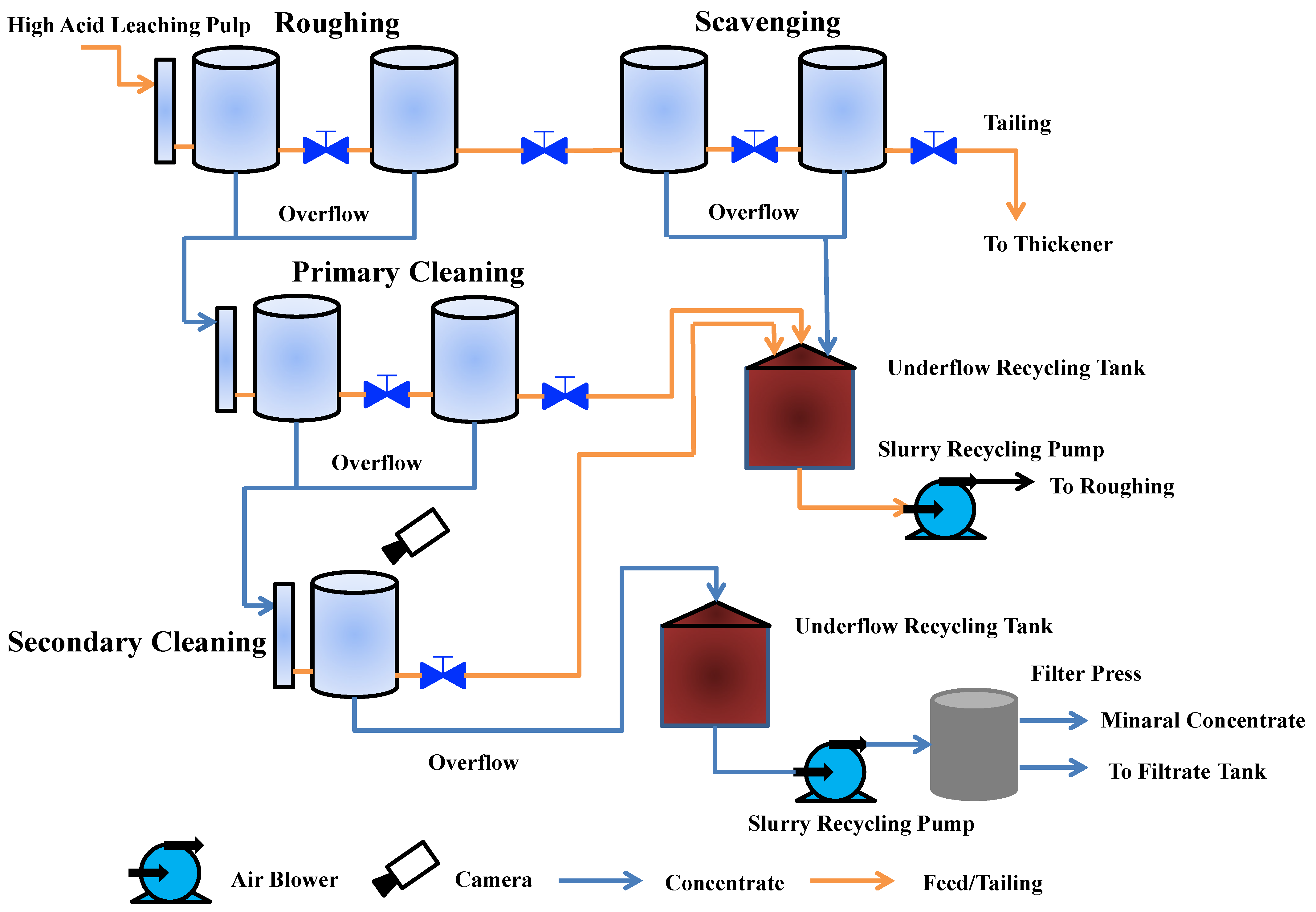
The aim of the mineral flotation process is to separate valuable minerals from useless materials or other minerals so as to obtain upgraded minerals. The concentrate grade is measured by calculating the percentage of the recovered useful element mass in the total concentrate mass. As a key performance indicator to evaluate the flotation effect in metallurgical enterprises, the concentrate grade directly reflects the quality of flotation working conditions. When the grade of the concentrate is too low, the working conditions of the flotation process will be in an abnormal state. The operator should adjust the flotation operating variables such as the inlet air flow and pulp level, related to the flotation working conditions in order to improve the concentrate grade. The better the flotation working conditions, the higher the concentrate grade. Thus, the concentrate grade reflects the flotation working conditions.

In the process of mineral flotation, the process working conditions are judged mainly according to the color, size and other features of the flotation froth, and operating parameters such as the air blowing amount are adjusted to ensure that the concentrate grade reaches the standard. Due to strong subjective and labor-intensive manual control, the efficiency of production is low, and the grade of the concentrate cannot be guaranteed. Therefore, researchers have studied the features of flotation froth images and found that the image features of mineral flotation froth are closely related to the operating parameters, working conditions and concentrate grade in the flotation process. Researchers continue to obtain shallow features, such as the color, texture and size of mineral flotation froth images, through image processing technology to identify the working conditions of the flotation process [1,2,3,4,5,6] and realize the optimal control of the flotation process. The extracted flotation froth image features, however, contain an excessive amount of redundant and noisy information, resulting in the low accuracy of working condition recognition and affecting flotation production efficiency. Therefore, it is of great significance to achieve the optimal control of the flotation process and improve the mineral flotation concentrate grade by studying a more effective mineral flotation process working condition recognition method.

The key to realizing the optimal control of the flotation process is the accurate extraction of flotation froth image features. Therefore, researchers are committed to extracting the features of flotation froth images and identifying the working conditions of the flotation process on this basis [7,8,9,10]. Such features include the following.

The color of the froth can reflect the types of particles carried by the froth and the quality of the flotation working conditions during the flotation process. In the past, many researchers have described color information mainly by calculating statistics such as the mean and standard deviation of each component of the color space, such as RGB, HSV and HIS [11,12,13]. However, the extraction of color information is susceptible to lighting.

The texture of the froth, which is primarily represented by calculating the arrangement rules and local patterns of the local gray value of the image, partially reflects the quality of the flotation process. In the past, domestic and foreign researchers extracted the texture features of flotation froth mainly by using the gray-level co-occurrence matrix (GLCM) [14], wavelet transform [15] and texture spectrum [16]. The GLCM describes the texture features through the calculation of second-order statistics in all directions, leading to the problem that high-dimensional matrices are computationally intensive, and it is difficult to completely describe the froth texture features through single-direction statistics. The color information is not taken into account when extracting froth texture features using the wavelet transform and texture spectrum, and the texture is instead described by conventional statistics (such as uniformity, entropy, etc.), which makes it difficult to completely and accurately represent the local differences in the froth image texture under various working conditions.

The working conditions of the flotation process can also be reflected by the size features of the froth, which mainly include the average size and deflection of the froth [17]. Beginning with the accurate segmentation of the froth image, froth size features can be accurately acquired. In the past, researchers have conducted extensive research on froth segmentation methods, including threshold segmentation [18], watershed segmentation [19] and valley edge detection [20], three widely used froth image segmentation methods in the flotation process. According to the features of flotation froth images, researchers concluded that the watershed segmentation algorithm is suitable for segmenting mineral flotation froth images among many segmentation algorithms. However, the traditional watershed segmentation algorithm is prone to over-segmentation or under-segmentation. 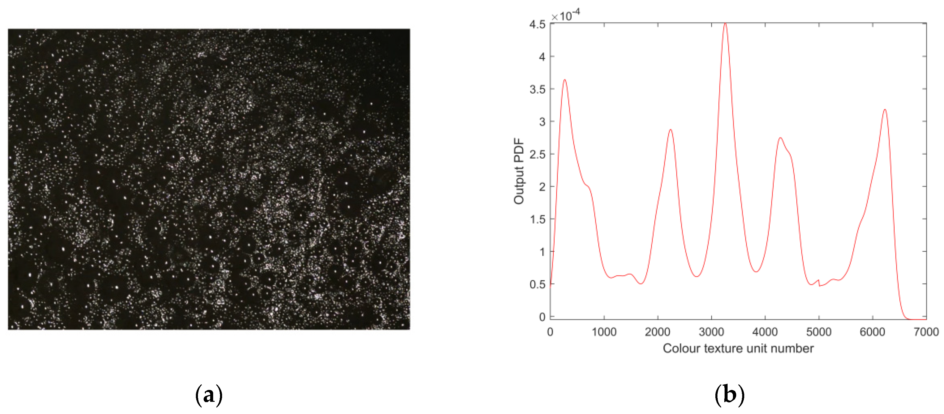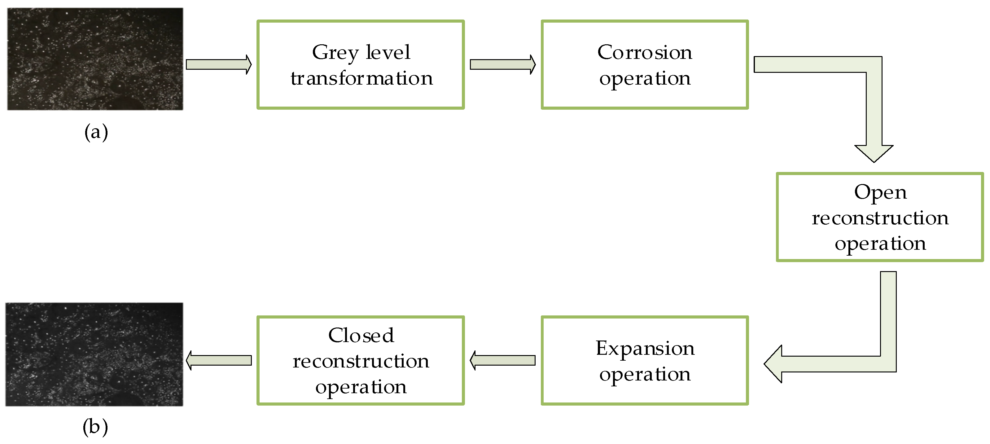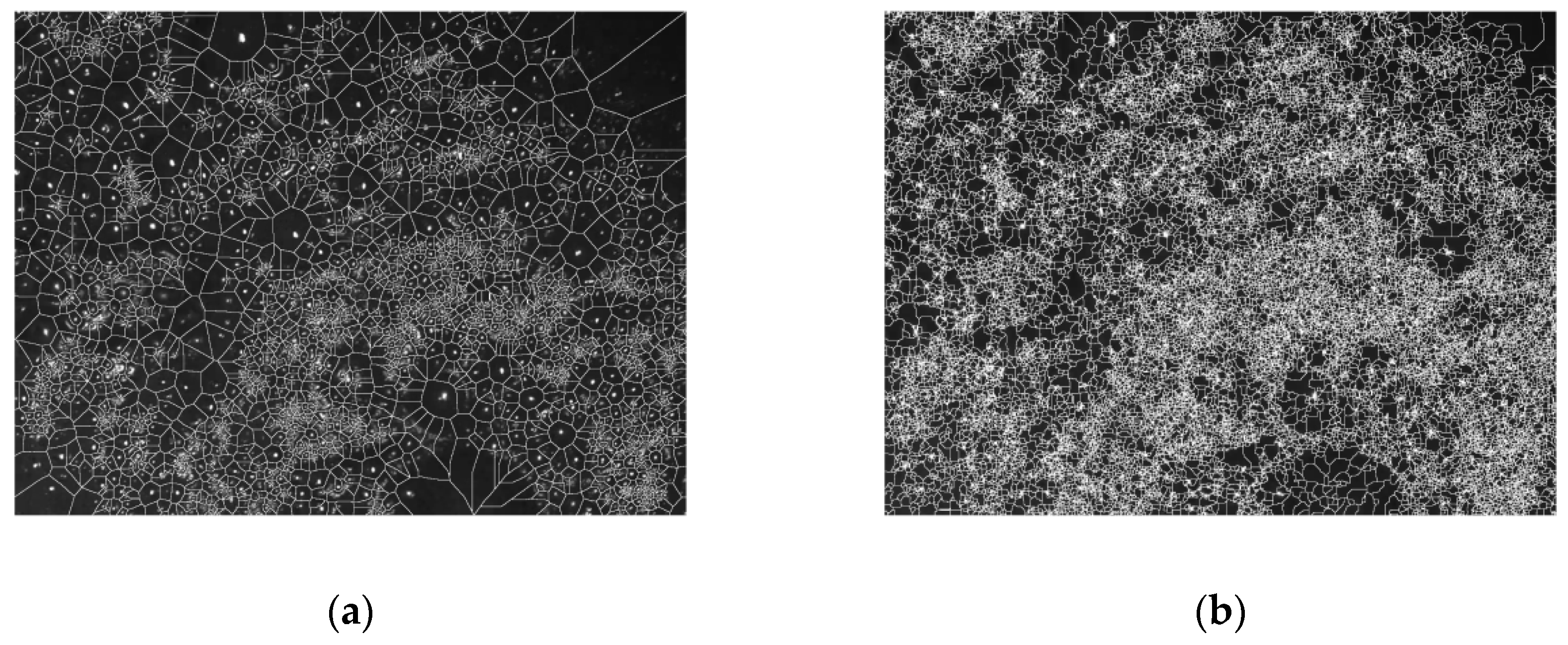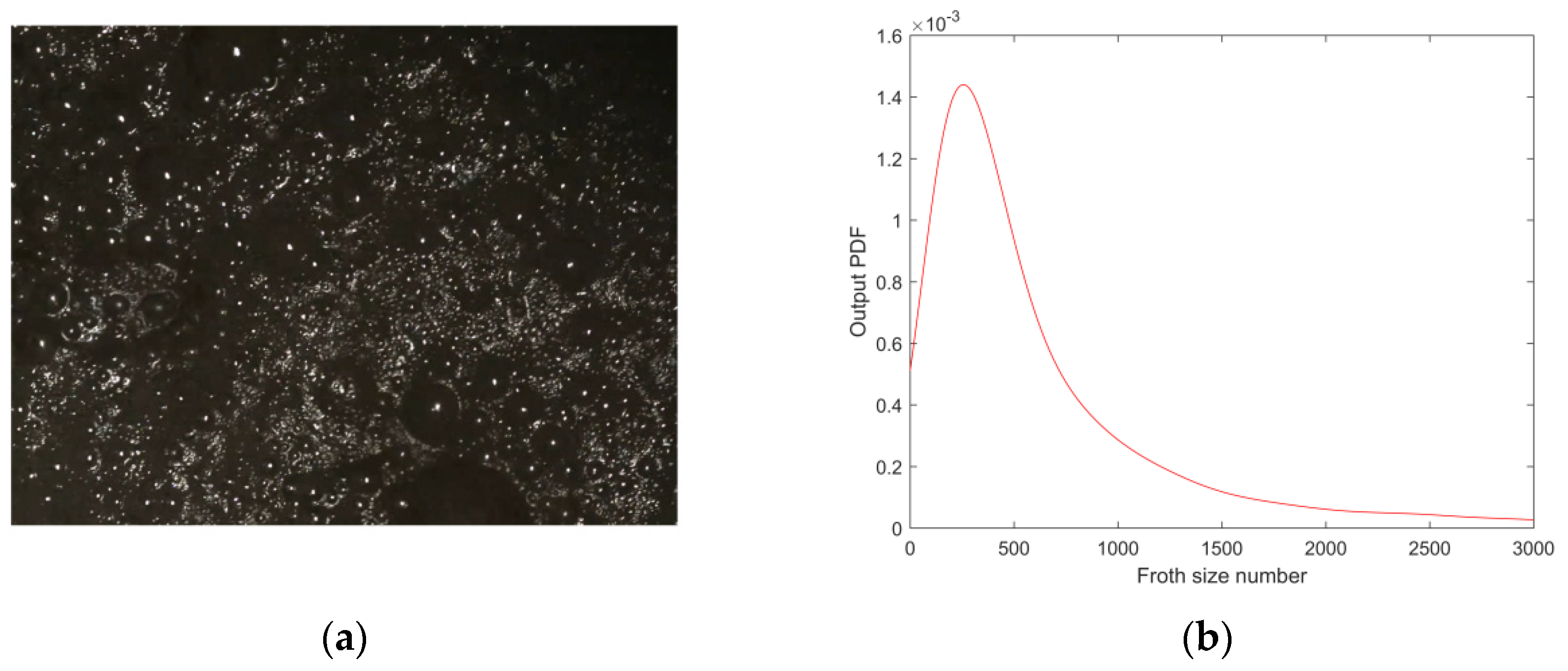Therefore, researchers subsequently improved the watershed segmentation algorithm to promote the accuracy of flotation froth image segmentation and solved this problem to a certain extent [21,22,23,24]. In order to accurately extract the size features of flotation froth, further improvements are needed in the segmentation of mineral flotation froth images. The size features of the froth image are extracted after the froth image segmentation of mineral flotation has been completed. In previous studies, when extracting the size features of froth images, most post-processing analyses only extracted single-valued features, such as the mean, variance and peak value of the froth size, while ignoring the overall distribution of the froth size.

Since flotation froth contains a large amount of information reflecting flotation conditions, scholars, both domestically and internationally, have conducted a great number of studies on the detection of flotation process working conditions based on froth image features [25,26]. Zhu et al. [27] proposed a flotation working condition recognition method using an LVQ neural network and a rough set on the basis of extracting froth texture features. Xu et al. [28] proposed a fault detection method, which realizes the fault detection and diagnosis of the flotation process by detecting the filter based on the output probability density function and Lyapunov stability analysis. Zhao et al. [29] proposed a fault working condition identification method for the antimony flotation process based on multi-scale texture features and embedding prior knowledge of the K mean. By first extracting features from the flotation froth image and then feeding the generated feature vectors to the classifier, these techniques enable the recognition of the flotation process working conditions. The results demonstrate that these methods can identify the working conditions of the flotation process to a certain extent. However, excessive are included in the extracted features, which affects the accuracy of recognition. Deep learning networks can now automatically extract deep features from image data with better flexibility and classification ability, so researchers have begun to use deep learning networks to identify the working conditions of the flotation process [30,31,32]. Fu et al. [33] used convolutional neural networks for pre-training on image databases of common objects for extracting features from flotation froth images and then effectively identified the working conditions of the mineral flotation process. Zarie et al. [34] studied convolutional neural networks to classify froth images collected from industrial coal flotation towers operating under various process working conditions. Fu et al. [35] solved the problem that deep learning network training requires a large number of flotation image datasets using transfer learning and network retraining. A large number of studies have proved that the method of identifying working conditions in the mineral flotation process based on deep learning network is effective [36,37,38].

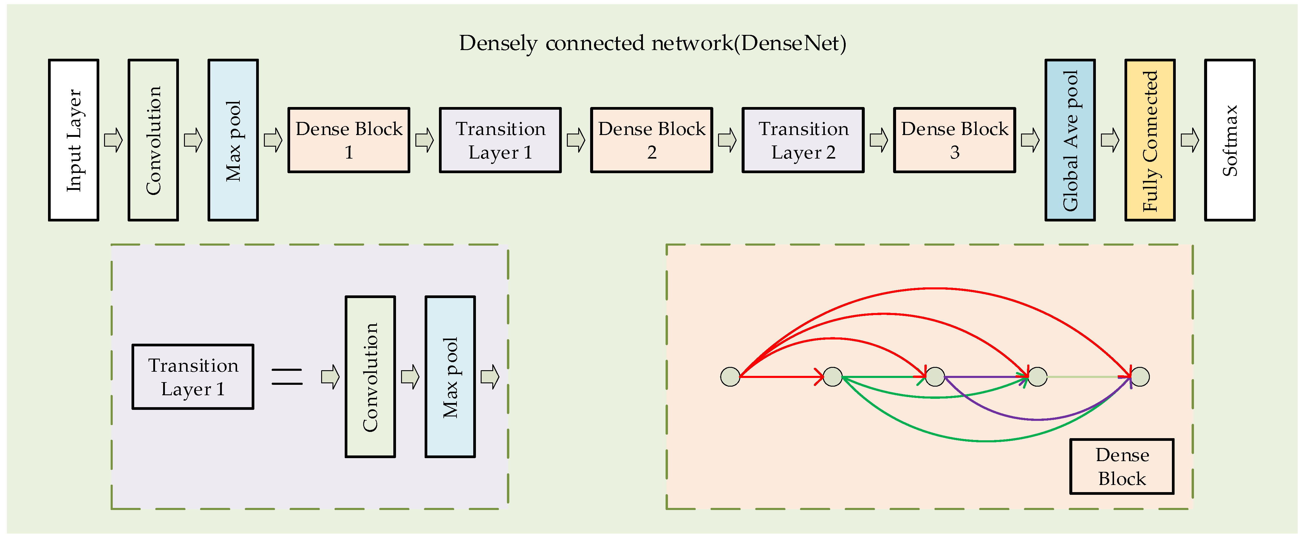
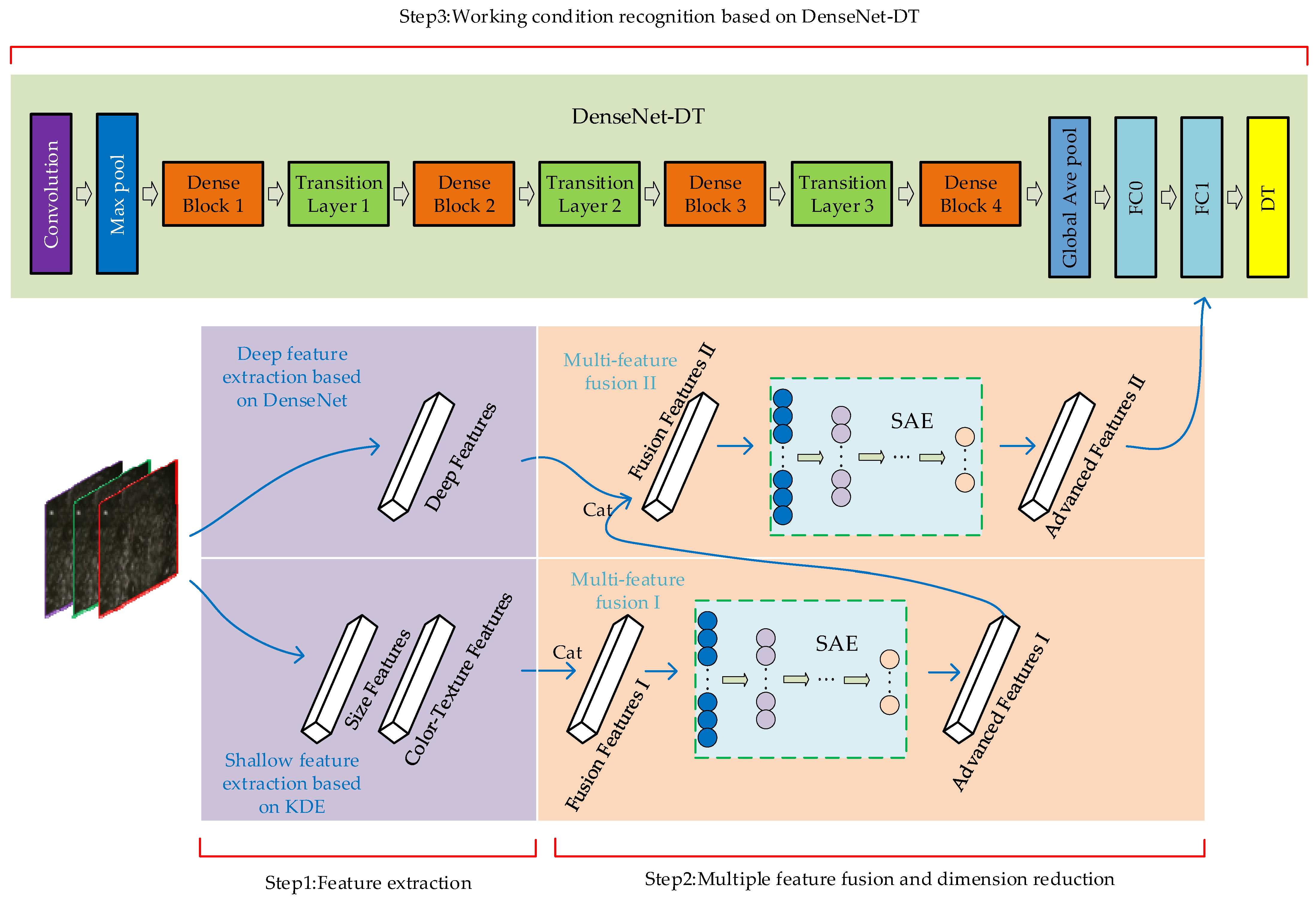
In order to solve the problem that the features extracted by the traditional flotation process working condition recognition method are not comprehensive and contain excessive redundant information and noisy information, a novel recognition method based on DSFF-DenseNet-DT is proposed in this paper. It can effectively identify the working conditions of the mineral flotation process. Firstly, the shallow features (color texture features and size features) and deep features of the froth images based on nonparametric kernel density estimation and DenseNet are extracted, solving the problem that the extracted froth features are not detailed and comprehensive. The extracted shallow features and deep features are then fused and reduced based on the Cat-SAE two-stage feature fusion method, which solves the problem that the extracted froth features have more redundant information and noisy information. Finally, the classification layer of DenseNet is replaced with a decision tree to obtain DenseNet-DT for working condition recognition. Compared with DenseNet, it improves the accuracy of working condition recognition. The main contributions of this paper are summarized as follows:

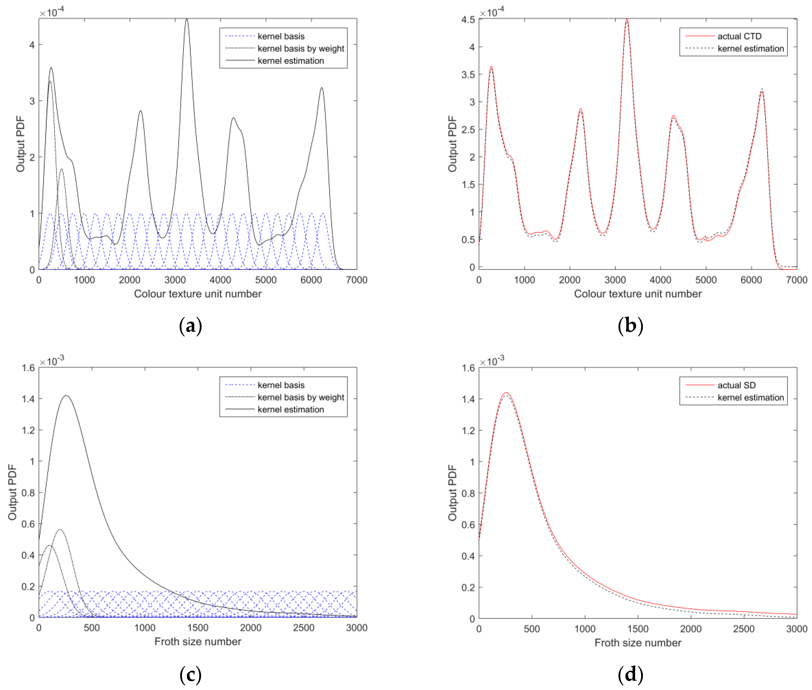
• A deep and shallow feature extraction method based on nonparametric kernel density estimation and DenseNet is proposed. The color texture, size and other detail features of the froth image are extracted effectively.
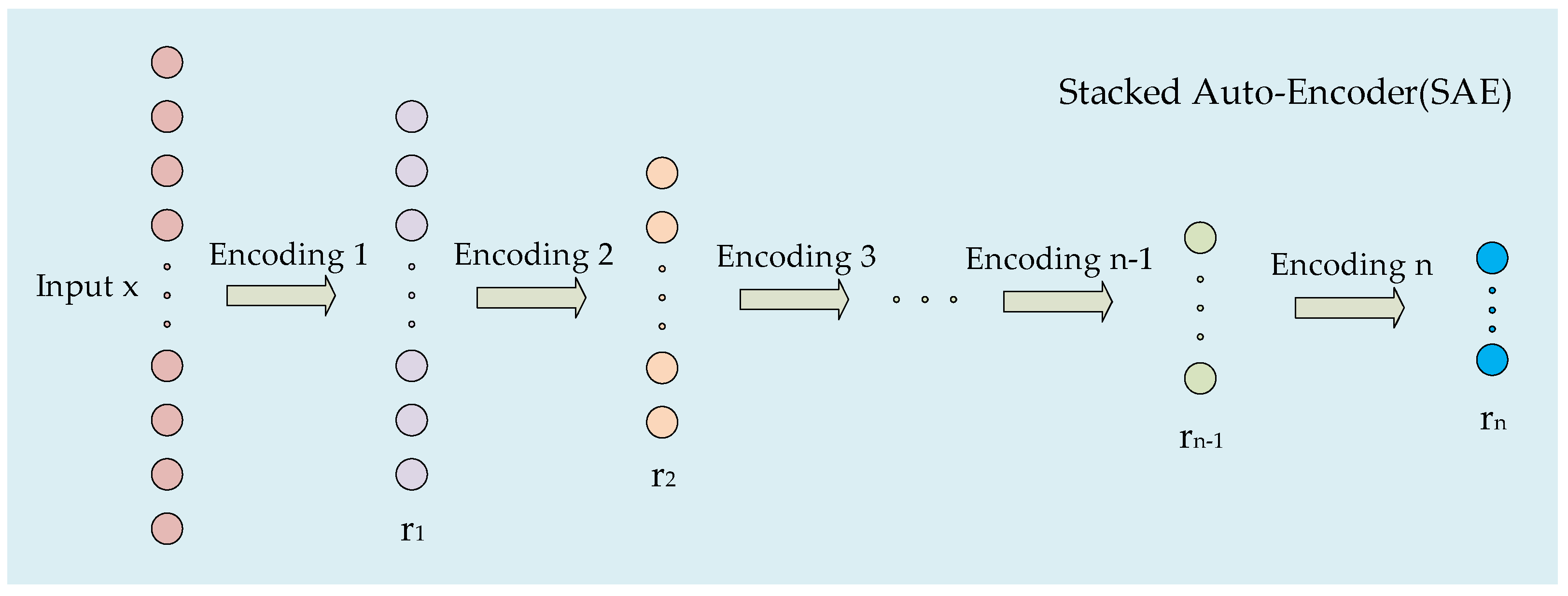
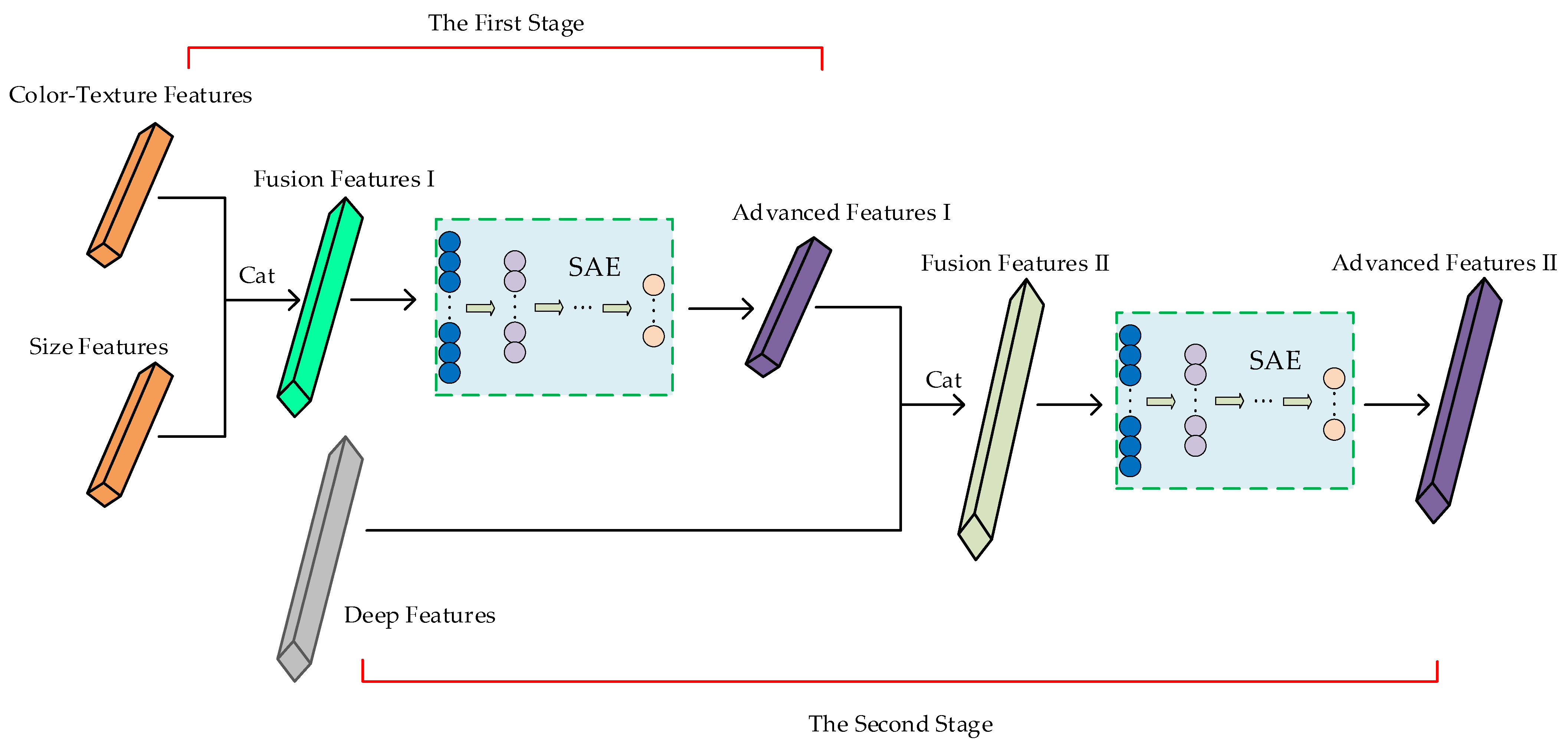
• A two-stage multi-feature fusion method based on Cat-SAE is proposed. The shallow features of the froth image are fused with deep features, comprehensively describing the feature information and eliminating feature redundancy and noise.
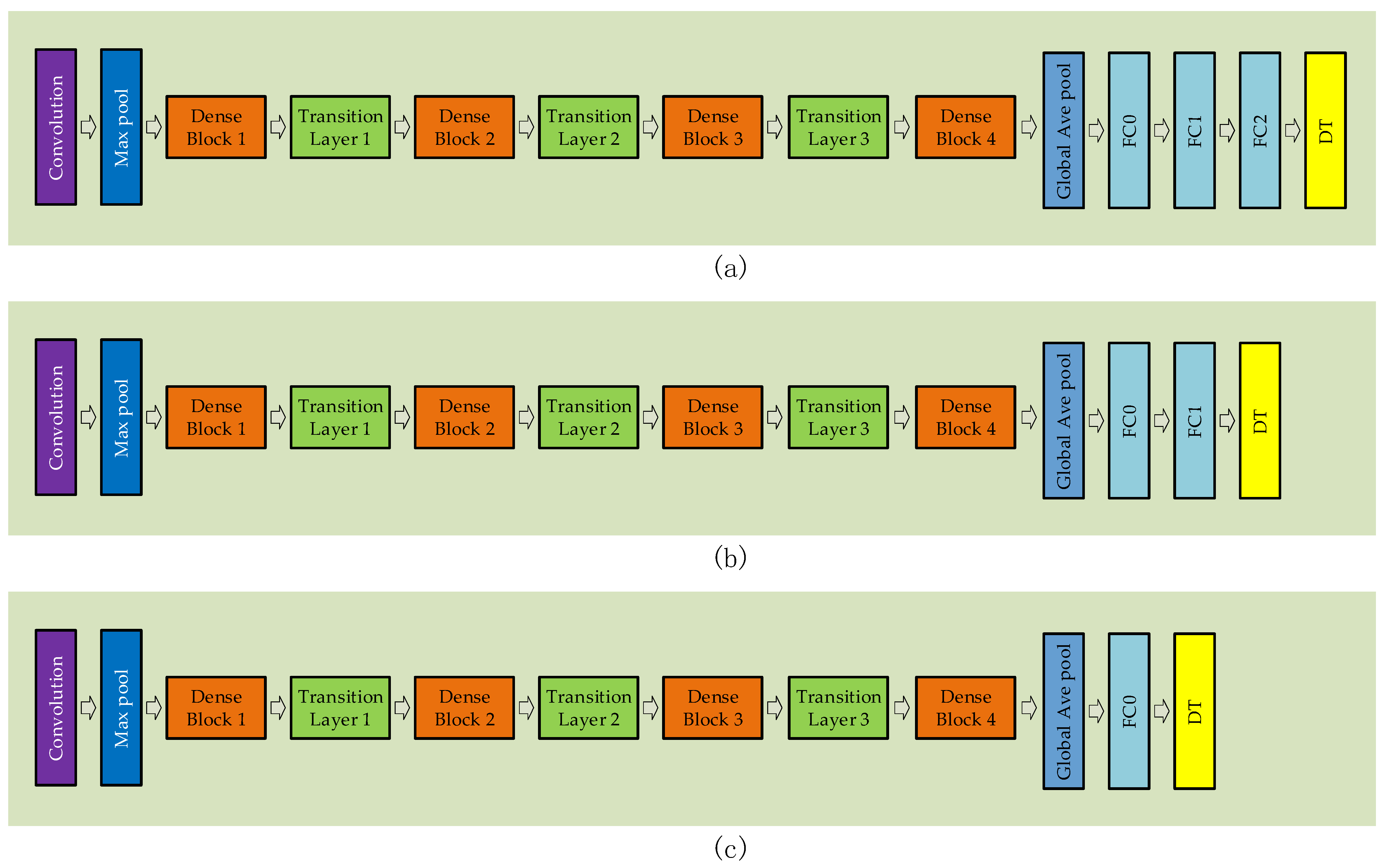
• A working condition recognition method based on DenseNet-DT is proposed, which replaces the classification layer of DenseNet with DT to obtain DenseNet-DT. It can effectively identify the flotation process working conditions.

This paper’s structure is summarized as follows. The theoretical context is introduced in Section 2. Section 3 introduces the proposed method as well as the detailed framework. Section 4 presents the experimental findings and analysis. Section 5 contains the conclusion.

2. Theoretical Background

2.1. Nonparametric Kernel Density Estimation

Kernel density estimation is a nonparametric method for estimating the probability density function. $X_1,X_2,\cdots ,X_n$ are $n$ sample points of an independent and homogeneous distribution, and their probability density is $f$; its kernel density estimation can be calculated by the following equation:

$${\widehat{f}}_{ker}\left(x\right)=\frac{1}{n}{\displaystyle \sum }_{i=1}^n{K}_h\left(x-X_i\right)=\frac{1}{nh}{\displaystyle \sum }_{i=1}^{n}K\left(\frac{x-X_i}{h}\right)$$

(1)

where ${\widehat{f}}_{ker}\left(x\right)$ is the estimated probability density function, and $K\left(\frac{x-X_i}{h}\right)$ is the $i$th kernel function and satisfies $\int K\left(\frac{x-X_i}{h}\right)dt=1$ to ensure the true density estimation. $h$ is the smoothing parameter (bandwidth) of the kernel function.

2.2. Densely Connected Network

DenseNet is a convolutional neural network developed by Huang et al. [39]. It is mostly made up of dense blocks, transformation layers and fully connected layers, in which the dense blocks contain multiple bottleneck layers, the bottleneck layer is made up of two convolutional layer connections with convolutional kernel sizes of 1 and 3, respectively, and the transformation layer consists of a convolutional layer with a convolutional kernel size of 1 and an average pooling layer with a stride size of 2. The network structure of DenseNet is shown in Figure 1.

A different connection mode is proposed in DenseNet to introduce direct connections from any layer to all subsequent layers, which is implemented in a dense block. The feature maps of the first $\ell -1$ layer are $X_0,X_1,\cdots ,X_{\ell -1}$, and the feature maps of the $\ell$ layer can be calculated by the following formula:

$$X_{\ell }=H_{\ell }\left(\left[X_0,X_1,\cdots ,X_{\ell -1}\right]\right)$$

(2)

where $H_{\ell }(.)$ is a composite function for three consecutive operations: BN, ReLU and a convolutional layer with a convolution kernel size of 3.

2.3. Stacked Autoencoder (SAE)

An encoder and decoder make up the unique neural network design known as the autoencoder (AE). The encoding process of raw data from the input layer to the hidden layer is given by the following equation:

$$r={\sigma }_1\left(W_{1}x+b_1\right)$$

(3)

where $x$ is the original high-dimensional input, and $r$ is the data representation of $x$ in the low-dimensional space. ${\sigma }_1\left(W_{1}x+b_1\right)$ is a nonlinear transformation of $x$.

The decoding process from the hidden layer to the output layer is given by the following equation:

$$\widehat{x}={\sigma }_2\left(W_{2}r+b_2\right)$$

(4)

where $\widehat{x}$ is the reconstruction output, and ${\mathsf{\sigma }}_2\left(W_{2}r+b_2\right)$ is a nonlinear transformation of $r$.

By reducing reconstruction mistakes, AE reconstructs data. The formula to minimize the reconstruction error is as follows:

$$\theta =\arg \underset{\theta }{\min }L\left(X,Z\right)=\arg \underset{\theta }{\min }\frac{1}{2}{\displaystyle \sum }_{i=1}^N\Vert x^{\left(i\right)}-z{(x^{\left(i\right)})}^2\Vert$$

(5)

where X is the raw input, and Z is the output of the AE.

SAE is obtained by first removing the output layer after training a single AE and then using $r$ as the original input information to train a new AE. When multiple AEs are stacked, the structure of the resulting SAE is shown in Figure 2. The output of SAE can be expressed as:

$$r_n={\sigma }_n\left(W_n{r}_{n-1}+b_n\right)\hspace{1em}n\ge 2$$

(6)

where $x$ is the original high-dimensional input, ${\mathsf{\sigma }}_n\left(W_n{r}_{n-1}+b_n\right)$ is a nonlinear transformation of $r_{n-1}$, and $r_n$ is the data representation of $x$ in the low-dimensional space after $n$ AE encoding.

2.4. Decision Tree (DT)

DT models can associate image features with labels. For a given dataset, DT is trained by starting from the root node of the entire prediction space. Classification rules and prediction models are applied at each node of the tree to minimize specific loss functions.

Consider the training set $D$ consisting of $N$ samples, where $D=\left\{\left(x_1,y_1\right),\left(x_1,y_1\right),\dots ,\left(x_n,y_n\right)\right\}$, $x$ represents the input, and $y$ represents the label. There are many attributes in $x$, with the attribute set $A=\left\{a_1,a_2,\dots ,a_m\right\}$, where $a$ represents a certain attribute, and $m$ represents the number of attributes. The DT model is trained using training set $D$ and attribute set $A$ as input.

The key to DT learning is determining how to select the optimal partition of attributes when training the DT model. Information entropy is used to divide attributes in this study. Suppose that the proportion of class $K$ samples in the current sample set $D$ is $P_k\left(k=1,2,\dots ,\left|y\right|\right)$; the information entropy of $D$ is defined as:

$$Ent\left(D\right)=-{\displaystyle \sum }_{k=1}^{\left|y\right|}{P}_k{\log }_2{P}_k$$

(7)

where the smaller the value of $Ent\left(D\right)$, the higher the purity of $D$.

The information gain is directly based on the information entropy to calculate the change in information entropy caused by the current partition. The information gain obtained by dividing sample set $D$ with attribute $a$ is:

$$Gain\left(D,a\right)=Ent\left(D\right)-{\displaystyle \sum }_{v=1}^V\frac{\left|D^v\right|}{\left|D\right|}Ent\left(D^v\right)$$

(8)

in which the value of discrete attribute $a$ is $\left\{a^1,a^2,\dots ,a^v,\dots ,a^V\right\}$, $a^v$ is the $v$th attribute value of attribute $a$, and there are $V$ attribute values in attribute $a$. The greater the information gain, the greater the purity gain obtained by using attribute $a$ for partitioning.

3. Proposed methodology

The three key steps of the DSFF-DenseNet-DT working condition recognition approach are depicted in Figure 3’s framework. The first step is feature extraction based on nonparametric kernel density estimation and DenseNet. The second step is the two-stage feature fusion dimensionality reduction based on Cat-SAE. The final step is the recognition of mineral flotation process working conditions based on DenseNet-DT. This section describes the implementation of DSFF-DenseNet-DT in order.

3.1. Feature Extraction

Under different working conditions, it is challenging to fully represent the local differences in the froth image texture using the current color texture feature description methods. The size feature extraction method only extracts the single-valued features of the froth size while ignoring the overall distribution of the froth size. The deep neural network can more effectively extract the detailed features of flotation froth images. Therefore, the shallow and deep features of mineral flotation froth images are obtained by nonparametric kernel density estimation and a deep neural network, respectively, which enables us to better identify the working conditions of the flotation process.

3.1.1. Shallow Feature Extraction Based on Nonparametric Kernel Density Estimation

CTD Feature Extraction

The GLCM and texture spectrum are the most common texture description methods, calculated based on gray-level images. It is difficult to accurately describe the texture features of froth using the GLCM method, and the texture spectrum method oriented to the number of texture units does not consider the color information. Therefore, He et al. [40] proposed the number of color texture units (CTUs) to describe CTD, which is defined as the PDF of the CTU number. This paper only improves the defined color variables based on the method proposed by He.

The froth images in the RGB color space are acquired from industrial field collection, while the HSV space can describe color information more closely to human vision. Therefore, the froth images are converted from the RGB color space to the HSV space, and the calculation formulas of H, S and V are as follows:

$$V=max$$

(9)

$$S=\left(max-min\right)/max$$

(10)

$$H=\{\begin{array}{l}60\left(G-B\right)/\left(max-min\right) if S\ne 0 and R=max\\ 120+60\left(B-R\right)/\left(max-min\right) if S\ne 0 and G=max\\ 240+60\left(R-G\right)/\left(max-min\right) if S\ne 0 and B=max\end{array}$$

(11)

where $max=max\left(R,G,B\right)$, and $min=min\left(R,G,B\right)$.

After converting the froth image to the HSV color space, the value of the color component H is mainly distributed between 0 and 90, and the value of the color component V is mainly distributed between 0 and 0.4. Therefore, the unequal interval quantification method is used to divide the three variables H, S and V into 34 (0–33), 10 (0–9) and 7 (0–6), respectively. Then, a new color variable is constructed:

C = 6H + 5S + 2V

(12)

where $C$ is an integer in [0,255].

Images of mineral flotation froths acquired online in the flotation cell are shown in Figure 4a. The CTD of the flotation froth image is obtained by calculating the frequency of the color texture unit number in the mineral flotation froth image, as shown in Figure 4b. It can be observed that the probability density distribution of the color texture unit number in the froth image is non-normal and multimodal.

SD Feature Extraction

It can be seen from the mineral flotation image that the mineral flotation images are almost entirely occupied by froth; the size, shape and grayscale of the froth are not uniform, and there are high bright spots reflected by light at the top of the froth. According to the characteristics of mineral flotation froth images, if the traditional watershed segmentation algorithm is used, over-segmentation or under-segmentation will occur. Therefore, an improved watershed segmentation algorithm is proposed to segment mineral flotation images.

Before segmenting the mineral flotation image, the froth image is preprocessed, and the preprocessing flow chart is shown in Figure 5. The image before preprocessing is shown in Figure 5a. Some isolated points in the original image are eliminated, and the processed image also becomes smoother after image preprocessing, which is conducive to the accurate segmentation of the flotation froth image. Figure 5b shows the processed image.

The structure element $b$ for the gray expansion and gray corrosion of image $f$ are denoted as $f\oplus b$ and $f\ominus b$, respectively, which are defined as follows:

$$\left(f\oplus b\right)\left(x,y\right)=\max \left\{f\left(x-x^{\prime },y-y^{\prime }\right)+b\left(x^{\prime },y^{\prime }\right)|\left(x^{\prime },y^{\prime }\right)\in D_b\right\}$$

(13)

$$\left(f\ominus b\right)\left(x,y\right)=\min \left\{f\left(x+x^{\prime },y+y^{\prime }\right)-b\left(x^{\prime },y^{\prime }\right)|\left(x^{\prime },y^{\prime }\right)\in D_b\right\}$$

(14)

where $D_b$ is the domain of $b$, and $f\left(x,y\right)$ is assumed to be $+\infty$ outside the domain of $f$.

If $\varrho$ is the mask and $f$ is the marker, the reconstruction of $\varrho$ from $f$ can be denoted as $R_{\varrho }\left(f\right)$, which is defined by the following iteration process:

• Step 1: Initialize ${\varphi }_1$ to tag image $f$;
• Step 2: Create the structural elements: $B=strel\left(‘dis{k}^{’},1\right)$;
• Step 3: Repeat ${\varphi }_{k+1}=\left({\varphi }_k\oplus B\right)\cap g$ until ${\varphi }_{k+1}={\varphi }_k$.
• Here, the marker $f$ must be a subset of $\varrho$, that is, $f\subseteq \varrho$.

The accurate segmentation of the flotation foam image is eventually obtained after image smoothing, along with distance transformation and the watershed segmentation algorithm with varied precision. The segmentation result of the flotation froth image is shown in Figure 6a. Figure 6b is the result of segmenting the flotation froth image using a classical watershed segmentation algorithm. It is clear that the improved watershed segmentation algorithm can segment the flotation froth image well, which is conducive to the accurate extraction of subsequent size features.

According to the principle of mathematical statistics, the size value of each segmented region is tallied after the froth image has been segmented, and the SD is described by the frequency of the size value of each region.

The image of the froth acquired online in the flotation cell is shown in Figure 7a. Figure 7b shows the SD of the flotation froth. It can be found from the figure that most froth sizes are small, and the froth SD span is large and presents a non-Gaussian distribution. The PDF curve of SD has a high peak value and large skewness, which has the characteristics of left skewness and a long tail.

CTD Feature Extraction

Supposing that the input of the mineral flotation dynamic system is $u\left(t\right)\in R^m$ and the output is $x\left(t\right)\in \left[a,b\right]$, the probability that the output $x\left(t\right)$ is in the range $\left[a,b\right]$ is defined as:

$$P\left(a\le x\left(t\right)\le b\right)={{\displaystyle \int }}_a^b{f}_{ker}\left(x,u\right)dx$$

(15)

where $f_{ker}\left(x,u\right)$ is the actual CTD or SD of the froth image.

The actual CTD and SD can be estimated by the following kernel density operators:

$${\hat{\mathrm{f}}}_{\ker }\left(\mathrm{x},\mathrm{u}\right)=\frac{1}{\mathrm{nh}}{\displaystyle \sum }_{\mathrm{i}=1}^{\mathrm{n}}\mathrm{K}\left(\frac{\mathrm{x}-{\mathrm{X}}_{\mathrm{i}}}{\mathrm{h}}\right)={\displaystyle \sum }_{\mathrm{i}=1}^{\mathrm{n}}{\mathrm{w}}_{\mathrm{i}}\mathrm{K}\left(\frac{\mathrm{x}-{\mathrm{X}}_{\mathrm{i}}}{\mathrm{h}}\right)$$

(16)

where ${\widehat{f}}_{ker}\left(x,u\right)$ is the approximate froth CTD function or SD function, and $K\left(\frac{x-X_i}{h}\right)$ is the $i$th kernel function and satisfies $\int K\left(\frac{x-X_i}{h}\right)dt=1$ to ensure true density estimation. $w_i$ is the weight corresponding to the $i$th kernel function, and $h$ is the bandwidth of the kernel function.

The normal kernel function was chosen to estimate the kernel density of the CTD PDF and SD PDF of the froth based on the features of the CTD and SD of mineral flotation froth.

Based on the normal kernel function prototype, a fitting kernel function suitable for mineral flotation froth CTD and SD is constructed as:

$$\mathrm{K}\left(\frac{\mathrm{x}-{\mathrm{X}}_{\mathrm{i}}}{\mathrm{h}}\right)=\frac{1}{\mathrm{h}\sqrt{2\mathsf{\pi }}}\exp \left(\frac{-{\left(\frac{\mathrm{x}-{\mathrm{X}}_{\mathrm{i}}}{\mathrm{h}}\right)}^2}{2}\right)\hspace{1em}-\infty <\frac{\mathrm{x}-{\mathrm{X}}_{\mathrm{i}}}{\mathrm{h}}<+\infty$$

(17)

where $X_i$ is the center of the $i$th kernel function along the horizontal axis.

Hypothesis:

$${\mathrm{K}}_0\left(\mathrm{z}\right)={\left[{\mathrm{k}}_1\left(\mathrm{z}\right),{\mathrm{k}}_2\left(\mathrm{z}\right),\cdots ,{\mathrm{k}}_{\mathrm{n}-1}\left(\mathrm{z}\right)\right]}^{\mathrm{T}}$$

(18)

$$\mathrm{W}\left(\mathrm{t}\right)={\left[{\mathrm{w}}_1\left(\mathrm{u}\right),{\mathrm{w}}_2\left(\mathrm{u}\right),\cdots ,{\mathrm{w}}_{\mathrm{n}-1}\left(\mathrm{u}\right)\right]}^{\mathrm{T}}$$

(19)

where $z=\frac{x-X_i}{h}$.

Since ${\int }_a^b{\widehat{f}}_{ker}\left(z,u\right)dz=1$, ${\int }_a^b{k}_i\left(z\right)dz=1$, $i=1,2,\cdots ,n$, $n-1$ weight coefficients are independent of each other. Thus, the CTD and SD models used can be written as follows:

$${\hat{\mathrm{f}}}_{\ker }\left(\mathrm{z},\mathrm{u}\right)={\mathrm{K}}^{\mathrm{T}}\left(\mathrm{z}\right)\mathrm{W}\left(\mathrm{t}\right)+\mathrm{g}\left(\mathrm{W}\left(\mathrm{t}\right)\right){\mathrm{k}}_{\mathrm{n}}\left(\mathrm{z}\right)$$

(20)

where $K\left(z\right)=K_0\left(z\right)$, $g\left(W\left(t\right)\right)=1-\sum _{i=1}^{n-1}{w}_i\left(u\right)$, and $g\left(W\left(t\right)\right)$ is the weight coefficient corresponding to the kernel function $k_n\left(z\right)$.

Several kernel functions were selected to describe the CTD and SD of froth according to the range of the number of froth color texture units and size values. Twenty-five kernel functions with a bandwidth of 120 are used to approximate the actual CTD curve, as shown by the blue dashed line in Figure 8a. Thirty kernel functions with a bandwidth of 120 are used to estimate the actual SD curve, as shown by the blue dashed line in Figure 8c. The two black dashed lines in Figure 8a,c represent the first and second kernel functions multiplied by the corresponding weight coefficients. The actual CTD and SD of the froth image are plotted as solid lines in Figure 8b,d. Figure 8b,d show the kernel density estimates of the actual CTD and SD of approximate froth images with dashed lines. The results suggest that the kernel density estimation can complete the description of the probability density distribution of the number of the froth color texture units and the probability density distribution of size values with a generally low feature dimension and high precision.

3.1.2. Deep Feature Extraction Based on DenseNet

Compared with the traditional two-stage working condition recognition method, which first carries out feature engineering and then identifies working conditions, a better method is to directly and automatically guide the feature extraction process according to the prediction ability of the model itself. Fu et al. [33] have shown that supervised feature extraction can produce better results than can be achieved without directly extracting features to achieve the same goal. Additionally, it also illustrates that overfitting the model due to too little data can be prevented by pre-training deep learning networks using image data from different domains.

DenseNet was used to extract the deep features of froth images. The two fully connected layers fc1 and fc2 are added after the fully connected layer fc0 of the DenseNet121 network, and their parameters are shown in

Table 1. Parameters of the DenseNet fully connected layer.

Layers	Input Features	Output Features
fc0	1024	1000
fc1	1000	512
fc2	512	4

. The fully connected layer fc2 is connected to the classification layer.

We first pre-trained DenseNet on the CIFAR10 dataset and then trained it on the flotation froth image dataset.

Table 2. Hyperparameter settings during model training.

Input_size	Batch_size	Epoch	Optimizer	Learning_rate	Momentum	Weight_decay
224 $\times$ 224	32	30	SGD	0.001	0.9	0.001

describes the settings of hyperparameters during training. The froth image is automatically resized to 224 $\times$ 224 pixels after the network has been trained to extract features from the froth image. Three feature vectors with dimensions of 1 $\times$ 1000, 1 $\times$ 512 and 1 $\times$ 4 are obtained by recording the node output of the fully connected layer. No parameters of the network are tuned except for the output layers that are input to different sets of labels. Finally, the classification layer is removed and replaced with a DT model.

3.2. Two-Stage Feature Fusion Based on Cat-SAE

The feature fusion method serves a vital role in the field of pattern recognition. The fused features retain the necessary and significant information, reducing the redundancy and noise of the original data. The fusion of the extracted features can achieve the complementary advantages of multiple features, and more robust and accurate recognition results can be obtained. The Cat-SAE two-stage feature fusion method was adopted in this study, and the fusion process is shown in Figure 9.

The first stage is the fusion of shallow features. First, the Concat operation is used to fuse the color texture features and size features to obtain features with more useful information. Then, SAE is applied to reduce the dimensionality of the fused features to obtain more abstract high-level features.

The second stage is to fuse the fused shallow features with deep features. First, the Concat operation is used to fuse the fused shallow features with deep features. Then, SAE is employed to reduce the dimensionality of the fused features.

The changes in feature dimensions in two-stage feature fusion based on Cat-SAE are shown in

Table 3. The changes in feature dimensions during the two-stage multi-feature fusion process based on Cat-SAE.

Features to Be Used		Fusion1	Advanced1	Features to Be Used		Fusion2	Advanced2
CT_Features	S_Features			Advanced1	D_Features
25	30	55	15	15	512	527	205

.

3.3. Working Condition Recognition Based on DenseNet-DT

Figure 1 shows that the classification layer in the DenseNet structure is softmax, which is linked to the fully connected layer. The classification softmax layer is replaced with DT to obtain the DenseNet-DT network structure in this study.

DenseNet-DT is formed by connecting DT to any fully connected layer of DenseNet. DenseNet-DT contains three structures, as depicted in Figure 10, as a result of the upgraded DenseNet having three fully connected layers. The structure when DT is connected to fc2 is shown in Figure 10a, the structure when connected to fc1 is shown in Figure 10b, and the structure when connected to fc0 is shown in Figure 10c. We conducted multiple rounds of training and testing on these three DenseNet-DT structures and determined the network structure finally used for flotation process working condition recognition through the test results.

4. Discussion

This section will verify the performance of the proposed DSFF-DenseNet-DT method in identifying mineral flotation process working conditions. According to the experimental findings, DSFF-DenseNet-DT has strong robustness and can detect mineral flotation working conditions more accurately than other recognition methods. This section includes the experimental environment and datasets and performance analysis.

4.1. Experimental Environment and Datasets

The hardware platform implemented in the experiment is as follows: the CPU is Inter(R) Core(TM) i9-9980XE, 3.00GHz, the GPU is NVIDIA GeForce RTX 2080Ti, and RAM is 64GB. The software runs on Windows 10 Professional Edition, Matlab2015a, Python 3.7 and Pytorch 1.9.0.

The flow chart of the mineral flotation process is shown in Figure 11. The flotation process is divided into roughing, cleaning and scavenging, and cleaning is further divided into primary and secondary cleaning. The high-acid-leaching pulp first enters the roughing separation process, and the overflow froth of roughing is sent to the two-level cleaning process. Then, the overflow froth of secondary cleaning is filtered through the compressor to obtain the final concentrate. The bottom pulp in the roughing process is discharged into the scavenging process to obtain tailings. The overflow froth of scavenging and the bottom pulp of two-level cleaning are returned to the roughing process for recycling. The camera was installed above the secondary cleaning tank to capture the froth images.

The dataset in this study was collected at a metallurgical plant site. The data acquisition device consists of an RGB camera with a resolution of 1280 $\times$ 960 and a 35 mm lens, a high-frequency light source, a cover hook to protect the camera from dust, acid fog and ambient light, and an optical fiber with a length of more than 200 m, which is used for signal communication to the industrial PC in the operating room. The camera is mounted vertically on the flotation cell to capture the flotation froth images at a rate of 15 frames/s. The dataset in this experiment consists of 750 mineral flotation images under four classes of working conditions (including 30 C1 images, 300 C2 images, 190 C3 images and 230 C4 images), and the ratio of the training set to test set is 8:2. Figure 12 shows the froth images corresponding to four typical working conditions in the mineral flotation process.

(1)

The image corresponding to working condition C1 has less visible froth and higher water content in the froth. Numerous white bright spots are reflected on the froth surface, and the concentrate grade is typically below 50%, as shown in Figure 12a.

(2)

The image corresponding to working condition C2 has more froth, and the size of the froth is not uniform. Small froth is mixed with some larger froth, the froth color is lighter, and the texture is more uniform. The concentrate grade is usually above 50% and below 60%, as shown in Figure 12b.

(3)

The image corresponding to working condition C3 has a uniform froth size and a relatively small size. The color is darker, and the texture is rougher. The concentrate grade is relatively normal, usually above 60% and below 70%, as shown in Figure 12c.

(4)

The image corresponding to working condition C4 has a smaller froth size. The froth color is very dark, and the texture is rough. The flotation working condition is better, and the concentrate grade is normally above 70%, as shown in Figure 12d.

To quantify the performance of the proposed and other methods in this study, four evaluation metrics were used, including the accuracy rate, precision rate, recall rate and F1 score.

The accuracy rate represents the percentage of the total samples that were predicted correctly, and the formula is as follows:

$$\mathrm{Accuracy}=\frac{\mathrm{TP}+\mathrm{TN}}{\mathrm{TP}+\mathrm{TN}+\mathrm{FP}+\mathrm{FN}}\times 100\%$$

(21)

where TP is the true positive class, TN is the true negative class, FP is the false positive class, and FN is the false negative class.

The precision rate represents the probability of actual positive samples among those predicted to be positive, and the formula is as follows:

$$\mathrm{Precision}=\frac{\mathrm{TP}}{\mathrm{TP}+\mathrm{FP}}\times 100\%$$

(22)

The recall rate represents the probability of being predicted as a positive sample for a sample that is actually positive, and the formula is as follows:

$$\mathrm{Recall}=\frac{\mathrm{TP}}{\mathrm{TP}+\mathrm{FN}}\times 100\%$$

(23)

The F1 score represents the harmonic average of the precision rate and recall rate, and the formula is as follows:

$$\mathrm{F}1 \mathrm{score}=\frac{2\times \mathrm{Precision}\times \mathrm{Recall}}{\mathrm{Precision}+\mathrm{Recall}}$$

(24)

4.2. Performance Analysis

This section will analyze the performance of DSFF-DenseNet-DT. We compare DSFF-DenseNet-DT with other methods.

4.2.1. Experimental Results of DSFF-DenseNet-DT

We experimented with the proposed DSFF-DenseNet-DT method to conduct ten experimental runs in order to avoid results obtained by chance in the experiment. The average value of ten experimental runs was taken as the final experimental result. In

Table 4. Experimental results of DSFF-DenseNet-DT.

Category	Number	Accuracy	Precision	Recall	F1 score
C1	6	100%	100%	100%	1
C2	60	92%	94.83%	92%	0.934
C3	38	89%	87.18%	89%	0.88
C4	46	96%	93.62%	96%	0.948
Total	150	92.67%	93.9%	94.2%	0.94

, the experimental findings are displayed. The DSFF-DenseNet-DT method can effectively identify flotation working conditions and has good robustness. Its average accuracy, precision and recall of flotation working condition recognition exceeded 92.67%, and the F1 score reached 0.94, of which the recognition accuracy, precision and recall of class C1 reached 100%, and the F1 score reached 1. Figure 13 shows the confusion matrix of DSFF-DenseNet-DT on a self-built dataset. The confusion matrix’s diagonal value is the biggest, as can be seen, indicating that DSFF-DenseNet-DT can accurately identify the flotation working conditions.

4.2.2. Comparative Experiment of DSFF-DenseNet-DT

The recognition results of color texture features for DT classification are displayed in

Table 5. Experimental results of CTD-DT using color texture features for DT classification.

Category	Number	Category				Accuracy	Precision	Recall	F1 score
		C1	C2	C3	C4
C1	6	4	0	0	2	66.7%	57.1%	66.7%	0.615
C2	60	0	48	10	2	80%	77.4%	80%	0.787
C3	38	1	11	23	3	60.5%	63.9%	60.5%	0.622
C4	46	2	3	3	38	82.6%	84.4%	82.6%	0.835
Total	150	7	62	36	45	75.3%	70.7%	72.45%	0.716

. The recognition results of the size features used for DT classification are shown in

Table 6. Experimental results of SD-DT using size features for DT classification.

Category	Number	Category				Accuracy	Precision	Recall	F1 score
		C1	C2	C3	C4
C1	6	4	1	0	1	66.7%	80%	66.7%	0.727
C2	60	1	44	4	11	73%	86.3%	73%	0.791
C3	38	0	6	27	5	71%	84.4%	71%	0.771
C4	46	0	0	1	45	98%	72.6%	98%	0.834
Total	150	5	51	32	62	80%	80.8%	77.25%	0.789

. The four performance indicators of the CTD-based DT (CTD-DT) method were 75.3%, 70.7%, 72.45% and 0.716, respectively. The four performance indicators of the SD-based DT (SD-DT) method were 80%, 80.8%, 77.25% and 0.789, respectively. The average recognition accuracy, precision and recall of CTD-DT and SD-DT methods are below 81%, the F1 score is below 0.8, and the recall of C2 and C3 classes is below that of C4, which implies that classes labeled C2 and C3 are easily misclassified into other classes. The findings above indicate that the method of extracting features by digital image processing technology cannot capture some of the detailed information required by the classifier, and the extracted features contain more redundancy and noisy information.

The experimental outcomes of DenseNet-DT are displayed in

Table 7. Experimental results of DenseNet-DT when DT is connected to different fully connected layers.

Fully Connected Layer	Accuracy	Precision	Recall	F1 score
fc0	82.7%	80.7%	75.4%	0.78
fc1	86%	79.6%	80.7%	0.801
fc2	64%	47.5%	49.4%	0.484

when DT is connected to various completely connected layers. It can be found that when DT is connected to fully connected layer fc2, the recognition accuracy, precision and recall are below 65%, and the F1 score is even below 0.5. Therefore, the working condition recognition method when DT is connected to fc2 is infeasible. DenseNet-DT offers the highest metrics when DT is connected to fully connected layer fc1, with an accuracy and recall of more than 80% and an F1 score of more than 0.8. As a result, DT is directly connected to DenseNet’s fully connected layer fc1 in the proposed DSFF-DenseNet-DT method, the structure of which is shown in Figure 10b.

As illustrated in Figure 14, DenseNet-DT is compared with CTD-DT and SD-DT methods in order to confirm that the deep learning network has a strong detail feature extraction capacity. Compared with the CTD-DT and SD-DT methods, the accuracy and average accuracy of C2 and C3 with the DenseNet-DT method were increased by at least 15%, 5% and 6%, respectively. Except for the precision of the DenseNet-DT method, which is slightly below that of the SD-DT method, the other three performance metrics are superior to those of the CTD-DT and SD-DT methods. This is sufficient evidence that the deep learning network has an excellent capability for extracting detailed picture features, and the deep learning network can adaptively extract the features required by the classification model to improve the recognition accuracy of the classification model.

The effectiveness and superiority of the proposed method are shown by comparing CTD-DT, SD-DT, DenseNet-DT and shallow-feature-fusion-based DT (SFF-DT) methods with DSFF-DenseNet-DT. The comparison outcomes are shown in

Table 8. Comparison of DSFF-DenseNet-DT with other different methods in terms of accuracy, precision, recall and F1 score.

Method	Accuracy	Precision	Recall	F1 Score
CTD-DT	75.3%	70.7%	72.45%	0.716
SD-DT	80%	80.8%	77.25%	0.789
DenseNet-DT	86%	79.6%	80.75%	0.802
SFF-DT	85.3%	84.7%	84.6%	0.847
DSFF-DenseNet-DT	92.67%	93.9%	94.2%	0.941

. It is easy to find that the DenseNet-DT method is superior to the CTD-DT and SD-DT methods. This is primarily due to the fact that deep neural networks are more effective at extracting certain features that help classifiers. We also found that the accuracy, precision and recall of the SFF-DT method all reached 84%, which was at least 5.3%, 3.9% and 7.35% higher than those of the other two methods, respectively. The F1 score reached 0.847, an improvement of at least 0.058. The SFF-DT method performs significantly better than CTD-DT and SD-DT. This is because when color textures and size features are fused, the fused features have more information that is useful for classifier classification. Finally, it can be found that DSFF-DenseNet-DT outperforms the other methods in four evaluation metrics: the accuracy, precision and recall are improved by at least 6.67%, 9.2% and 9.6%, and the F1 score is improved by at least 0.094. On the one hand, deep features can provide more detailed information to the classifier. On the other hand, multi-feature fusion can make each feature undergo complementary fusion and provide the classifier with more valuable data. Therefore, the proposed method DSFF-DenseNet-DT is effective for mineral flotation process working condition recognition and is superior in performance to other existing methods.

5. Conclusions

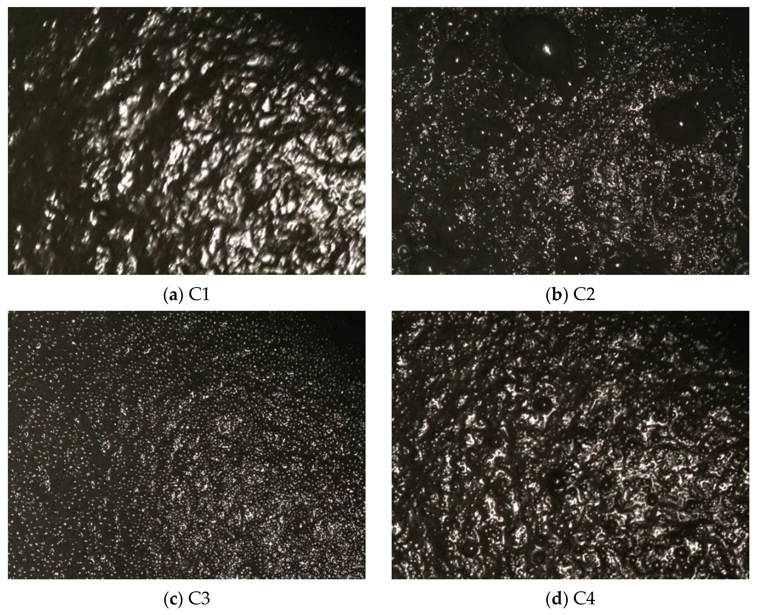
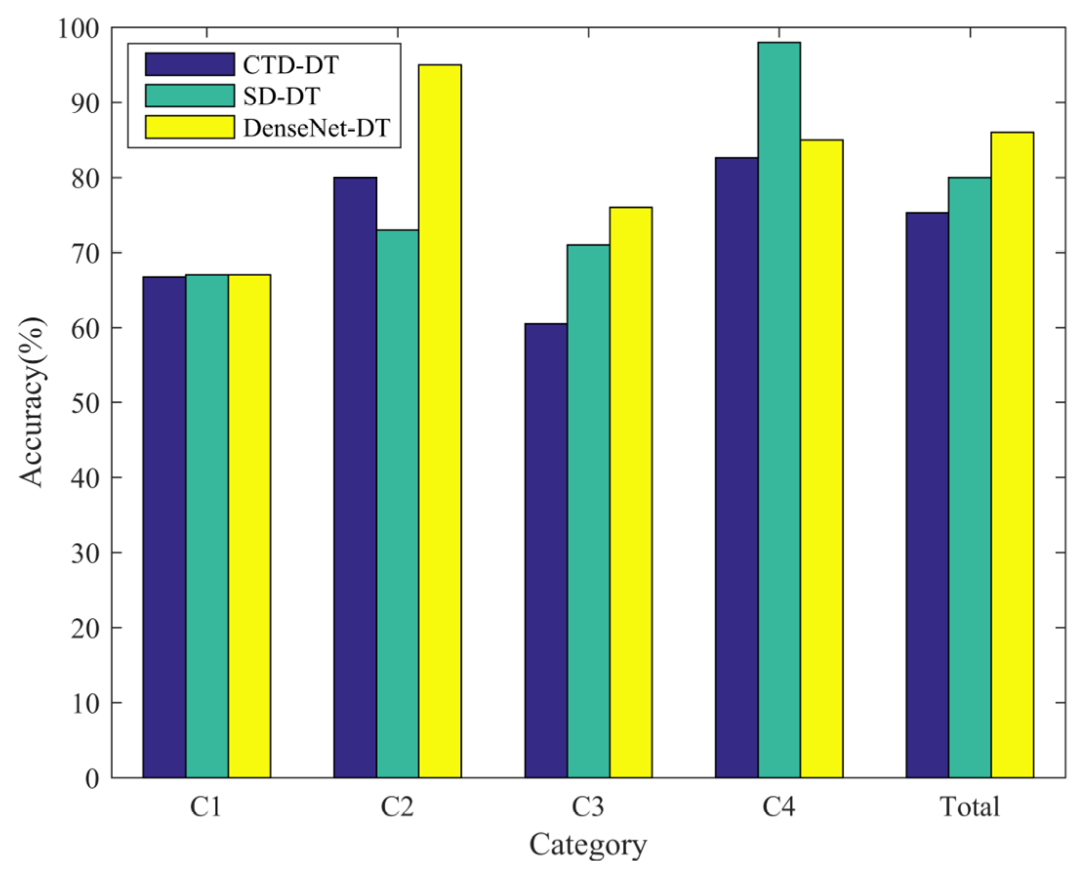
In this paper, a working condition recognition method based on DSFF-DenseNet-DT for the mineral flotation process is proposed, addressing the problem that the shallow features of flotation froth images extracted by digital image processing technology in the past contain excessive redundancy and noisy information. Through the two-stage feature fusion method based on Cat-SAE, extracted shallow features such as color texture and size are first fused to reduce dimensionality, and 15-dimensional fusion features are obtained. Then, the fused 15-dimensional features are fused with the deep features extracted by the deep neural network and reduced to obtain a 205-dimensional feature vector, and the fused features have less noisy information and redundant information. Finally, the fused features are fed into DenseNet-DT to achieve working condition recognition. Classification experiments were conducted by using flotation froth images acquired from industrial sites. Compared with the CTD-DT (75.3%) and SD-DT (80%) recognition methods, the recognition accuracy of DenseNet-DT (86%) has been greatly improved, demonstrating that detailed froth image features can be extracted more effectively using the deep learning network. Compared with other recognition methods, the recognition accuracy of SFF-DT (85.3%) and DSFF-DenseNet-DT (92.67%) is highly improved, indicating that the fusion and dimensionality reduction of features can eliminate redundant features and noisy information so as to improve the robustness of the model. The average recognition accuracy, precision, recall and F1 score of DSFF-DenseNet-DT can reach 92.67%, 93.9%, 94.2% and 0.94, respectively. It is able to accurately pinpoint the working conditions of the mineral flotation process, which is conducive to the optimization control of the flotation process and improves the grade of the concentrate.

References

1. Wang, W.X.; Li, L. Pattern recognition and computer vision for mineral froth. Int. Conf. Pattern Recognit. (ICPR’06) 2006, 4, 622–625. [Google Scholar] [CrossRef]
2. Ai, M.X.; Xie, Y.F.; Xie, S.W.; Gui, W.H. Shape-weighted bubble size distribution based reagent predictive control for the antimony flotation process. Chemom. Intell. Lab. Syst. 2019, 192, 103821. [Google Scholar] [CrossRef]
3. Ai, M.X.; Xie, Y.F.; Xu, D.G. Reagent Predictive Control Using Joint Froth Image Feature for Antimony Flotation Process. IFAC-Pap. 2018, 51, 284–289. [Google Scholar] [CrossRef]
4. He, Z.; Tang, Z.H.; Yan, Z.H.; Liu, J.P. DTCWT-based zinc fast roughing working condition identification. Chin. J. Chem. Eng. 2018, 8, 1721–1726. [Google Scholar] [CrossRef]
5. Harrave, J.M.; Hall, S.T. Diagnosis of concentrate grade and mass flowrate in tin flotation from colour and surface texture analysis. Miner. Eng. 1997, 10, 613–621. [Google Scholar] [CrossRef]
6. Liu, J.J.; MacGregor, J.F.; Duchesne, C.; Bartolacci, G. Flotation froth monitoring using multiresolutional multivariate image analysis. Miner. Eng. 2005, 18, 65–76. [Google Scholar] [CrossRef]
7. Moolman, D.W.; Aldrich, C.; Van, D.J.S.J.; Stange, W.W. Digital image processing as a tool for on-line monitoring of froth in flotation Plants. Miner. Eng. 1994, 7, 1149–1164. [Google Scholar] [CrossRef]
8. Wen, Z.P.; Zhou, C.C.; Pan, J.H.; Nie, T.C.; Jia, R.B.; Yang, F. Froth image feature engineering-based prediction method for concentrate ash content of coal flotation. Miner. Eng. 2021, 170, 107023. [Google Scholar] [CrossRef]
9. Gao, X.L.; Tang, Z.H.; Xie, Y.F.; Zhang, H.; Gui, W.H. A layered working condition perception integrating handcrafted with deep features for froth flotation. Miner. Eng. 2021, 170, 107059. [Google Scholar] [CrossRef]
10. Aldrich, C.; Avelar, E.; Liu, X. Recent advances in flotation froth image analysis. Miner. Eng. 2022, 188, 107823. [Google Scholar] [CrossRef]
11. Oestreich, J.M.; Tolley, W.K.; Rice, D.A. The development of a color sensor system to measure mineral compositions. Miner. Eng. 1995, 8, 31–39. [Google Scholar] [CrossRef]
12. He, M.F.; Sun, B. On-line froth depth estimation for sulphur flotation process with multiple working conditions. IEEE. Access 2019, 7, 124774–124784. [Google Scholar] [CrossRef]
13. Gui, W.H.; Liu, J.P.; Yang, C.H.; Chen, N.; Liao, X. Color co-occurrence matrix based froth image texture extraction for mineral flotation. Miner. Eng. 2013, 46–47, 60–67. [Google Scholar] [CrossRef]
14. Moolman, D.W.; Aldrich, C.; Van, D.J.S.J.; Stange, W.W. The classification of froth structures in a copper flotation plant by means of a neural net. Int. J. Miner. Process. 1995, 43, 193–208. [Google Scholar] [CrossRef]
15. Bartolacci, G.; Pelletier, P.; Tessier, J.; Duchesne, C.; Bossé, P.A.; Fournier, J. Application of numerical image analysis to process diagnosis and physical parameter measurement in mineral processes-Part I: Flotation control based on froth textural characteristics. Miner. Eng. 2006, 19, 734–747. [Google Scholar] [CrossRef]
16. Citir, C.; Aktas, Z.; Berber, R. Off-line image analysis for froth flotation of coal. Comput. Chem. Eng. 2004, 28, 625–632. [Google Scholar] [CrossRef]
17. Lin, B.; Recke, B.; Knudsen, J.K.H. Bubble size estimation for flotation processes. Miner. Eng. 2008, 21, 539–548. [Google Scholar] [CrossRef]
18. Moolman, D.W.; Aldrich, C.; Van, D.J.S.J.; Bradshaw, D.J. The interpretation of flotation froth surfaces by using digital image analysis and neural networks. Chem. Eng. Sci. 1995, 50, 3501–3513. [Google Scholar] [CrossRef]
19. Bonifazi, G.; Serranti, S.; Volpe, F.; Zuco, R. Characterisation of flotation froth colour and structure by machine vision. Comput. Geosci. 2001, 27, 1111–1117. [Google Scholar] [CrossRef]
20. Yang, C.H.; Xu, C.H.; Gui, W.H.; Zhou, K.J. Application of highlight removal and multivariate image analysis to color measurement of flotation bubble images. Int. J. Imaging Syst. Technol. 2009, 19, 316–322. [Google Scholar] [CrossRef]
21. Mehrshad, N.; Massinaei, M. New image-processing algorithm for bubble size distribution from flotation froth images. Miner. Metall. Process. 2011, 28, 146–150. [Google Scholar] [CrossRef]
22. Sadr-Kazemi, N.; Cilliers, J.J. An image processing algorithm for measurement of flotation froth bubble size and shape distributions. Miner. Eng. 1997, 10, 1075–1083. [Google Scholar] [CrossRef]
23. Jahedsaravani, A.; Massinaei, M.; Marhaban, M.H. An image segmentation algorithm for measurement of flotation froth bubble size distributions. Measurement 2017, 111, 29–37. [Google Scholar] [CrossRef]
24. Zhang, H.; Tang, Z.H.; Xie, Y.F.; Gao, X.L.; Chen, Q. A watershed segmentation algorithm based on an optimal marker for bubble size measurement. Measurement 2019, 138, 182–193. [Google Scholar] [CrossRef]
25. Aldrich, C.; Marais, C.; Shean, B.J.; Cilliers, J.J. Online monitoring and control of froth flotation systems with machine vision: A review. Int. J. Miner. Process. 2010, 96, 1–13. [Google Scholar] [CrossRef]
26. Ai, M.X.; Xie, Y.F.; Xie, S.W.; Li, F.B.; Gui, W.H. Data-driven-based adaptive fuzzy neural network control for the antimony flotation plant. J. Frankl. Inst. 2019, 356, 5944–5960. [Google Scholar] [CrossRef]
27. Zhu, J.; Wang, Y. Application of image recognition system in flotation process. In Proceedings of the 2008 7th World Congress on Intelligent Control and Automation (WCICA), Chongqing, China, 25–27 June 2008; pp. 6555–6659. [Google Scholar] [CrossRef]
28. Xu, C.H.; Gui, W.H.; Yang, C.H.; Zhu, H.Q.; Lin, Y.Q.; Shi, C. Flotation process fault detection using output PDF of bubble size distribution. Miner. Eng. 2012, 26, 5–12. [Google Scholar] [CrossRef]
29. Zhao, L.; Peng, T.; Zhao, L.; Xia, P.; Zhao, Y.H.; Song, Y.P. Fault Condition Recognition Based on Multi-scale Texture Features and Embedding Prior Knowledge K-means for Antimony Flotation Process. IFAC-Pap. 2015, 48, 864–870. [Google Scholar] [CrossRef]
30. Ai, M.X.; Xie, Y.F.; Tang, Z.H.; Zhang, J.; Gui, W.H. Deep learning feature-based setpoint generation and optimal control for flotation processes. Inf. Sci. 2021, 578, 644–658. [Google Scholar] [CrossRef]
31. Fu, Y.; Aldrich, C. Flotation froth image recognition with convolutional neural networks. Miner. Eng. 2019, 132, 183–190. [Google Scholar] [CrossRef]
32. Horn, Z.C.; Auret, L.; McCoy, J.T.; Aldrich, C.; Herbst, B.M. Performance of Convolutional Neural Networks for Feature Extraction in Froth Flotation Sensing. IFAC-Pap. 2017, 50, 13–18. [Google Scholar] [CrossRef]
33. Fu, Y.H.; Aldrich, C. Froth image analysis by use of transfer learning and convolutional neural networks. Miner. Eng. 2018, 115, 68–78. [Google Scholar] [CrossRef]
34. Zarie, M.; Jahedsaravani, A.; Massinaei, M. Flotation froth image classification using convolutional neural networks. Miner. Eng. 2020, 155, 106443. [Google Scholar] [CrossRef]
35. Fu, Y.; Aldrich, C. Using Convolutional Neural Networks to Develop State-of-the-Art Flotation Froth Image Sensors. IFAC-Pap. 2018, 51, 152–157. [Google Scholar] [CrossRef]
36. Olivier, L.E.; Maritz, M.G.; Craig, L.K. Estimating Ore Particle Size Distribution using a Deep Convolutional Neural Network. IFAC-Pap. 2020, 53, 12038–12043. [Google Scholar] [CrossRef]
37. Cen, L.H.; Wu, Y.M.; Hu, J.; Xie, Y.F.; Tang, Z.H. Application of density-based clustering algorithm and capsule network to performance monitoring of antimony flotation process. Miner. Eng. 2022, 184, 107603. [Google Scholar] [CrossRef]
38. Wang, X.; Zhou, J.W.; Wang, Q.K.; Liu, D.X.; Lian, J.M. An unsupervised method for extracting semantic features of flotation froth images. Miner. Eng. 2022, 176, 107344. [Google Scholar] [CrossRef]
39. Huang, G.; Liu, Z.; Maaten, L.V.D.; Weinberger, K.Q. Densely Connected Convolutional Networks. In Proceedings of the 2017 IEEE Conference on Computer Vision and Pattern Recognition (CVPR), Honolulu, HI, USA, 21–26 July 2017; pp. 2261–2269. [Google Scholar] [CrossRef] [Green Version]
40. He, M.F.; Yang, C.H.; Wang, X.L.; Gui, W.H.; Wei, L.J. Nonparametric density estimation of froth colour texture distribution for monitoring sulphur flotation process. Miner. Eng. 2013, 53, 203–212. [Google Scholar] [CrossRef]
Figure 1. Structure of DenseNet.
Applsci 12 12223 g001
Figure 2. Structure of SAE.
Applsci 12 12223 g002
Figure 3. The working condition recognition framework of DSFF-DenseNet-DT.
Applsci 12 12223 g003
Figure 4. (a) Mineral flotation froth images in flotation cell are collected online. (b) Color texture unit distribution of mineral flotation froth images.
Applsci 12 12223 g004
Figure 5. Flow chart of froth image preprocessing.
Applsci 12 12223 g005
Figure 6. (a) The segmentation result of the improved watershed segmentation algorithm. (b) The segmentation result of the traditional watershed segmentation algorithm.
Applsci 12 12223 g006
Figure 7. (a) Froth image acquired online by flotation cell. (b) SD of mineral flotation froth.
Applsci 12 12223 g007
Figure 8. (a) Gaussian kernel density estimation of froth color texture unit distribution. (b) Gaussian-kernel-based kernel density estimation method to estimate the actual color texture unit distribution. (c) Gaussian kernel density estimation of froth SD. (d) Gaussian-kernel-based kernel density estimation method to estimate the actual SD.
Applsci 12 12223 g008
Figure 9. The two-stage feature fusion process based on Cat-SAE.
Applsci 12 12223 g009
Figure 10. Structure of DenseNet-DT when DT is connected to different fully connected layers.
Applsci 12 12223 g010
Figure 11. The flow chart of mineral flotation process.
Applsci 12 12223 g011
Figure 12. Image of froth under four different typical working conditions.
Applsci 12 12223 g012
Figure 13. Confusion matrix of DSFF-DenseNet-DT on the self-built datasets.
Applsci 12 12223 g013
Figure 14. Comparison of CTD-DT, SD-DT and DenseNet-DT results.
Applsci 12 12223 g014