Two-View Mammogram Synthesis from Single-View Data Using Generative Adversarial Networks

Abstract

While two-view mammography taking both mediolateral-oblique (MLO) and cranio-caudual (CC) views is the current standard method of examination in breast cancer screening, single-view mammography is still being performed in some countries on women of specific ages. The rate of cancer detection is lower with single-view mammography than for two-view mammography, due to the lack of available image information. The goal of this work is to improve single-view mammography’s ability to detect breast cancer by providing two-view mammograms from single projections. The synthesis of novel-view images from single-view data has recently been achieved using generative adversarial networks (GANs). Here, we apply complete representation GAN (CR-GAN), a novel-view image synthesis model, aiming to produce CC-view mammograms from MLO views. Additionally, we incorporate two adaptations—the progressive growing (PG) technique and feature matching loss—into CR-GAN. Our results show that use of the PG technique reduces the training time, while the synthesized image quality is improved when using feature matching loss, compared with the method using only CR-GAN. Using the proposed method with the two adaptations, CC views similar to real views are successfully synthesized for some cases, but not all cases; in particular, image synthesis is rarely successful when calcifications are present. Even though the image resolution and quality are still far from clinically acceptable levels, our findings establish a foundation for further improvements in clinical applications. As the first report applying novel-view synthesis in medical imaging, this work contributes by offering a methodology for two-view mammogram synthesis.

1. Introduction

According to the World Health Organization (WHO), breast cancer was the world’s most prevalent cancer in 2020 [1,2]. A survey in the United Kingdom reported, in 2000, a five-year survival rate of 96.4% for women with early-stage breast cancer, which is similar to the rate for the general public [3]. This supports the idea that early detection is irrefutably crucial for addressing breast cancer. Screening mammography has contributed to the early detection and reduction in breast cancer mortality [4,5,6,7]. In many countries, two-view mammography presenting both mediolateral-oblique (MLO) and cranio-caudual (CC) views is the current standard method for examination in breast cancer screening [8,9]; however, single-view mammography using only the MLO view was mainly used in the early days of screening [4,5,8,10,11,12]. In some cases, especially for women under 50 years old in Europe and the United States (U.S.), single-view mammography is still performed. The reasons are attributed to the lower radiation dose, increased examination throughput, being less time- and cost-consuming, reduced overdiagnosis, and so on [8,10]. In Japan, the Ministry of Health, Labour, and Welfare updated their guidelines for breast cancer screening in 2004 [13], which state that women aged 40–49 years should be examined using two-view mammography, while that those aged 50 and older should be examined using single-view mammography. This is opposite to the situations in Europe and the U.S., where some women younger than 50 undergo single-view mammography. While breast cancer incidence is higher among older women in US, the incidence peaks in the 45–49 age group in Japan [14]. The differences in the age-specific incidences of this cancer affect the number of views required for screening mammography.

The important point is that CC-view mammograms are not necessarily obtained in breast cancer screening, whereas MLO-view mammograms must be taken. Unsurprisingly, the cancer detection rate with single-view mammography is inferior to those with two-view mammography [10,11,12,15], as the breast cancer may be visually obscured by overlapping mammary glands in two-dimensional mammograms [16]. Therefore, it is sometimes hard to distinguish the overlapped cancer from surrounding tissues, particularly in single-view mammograms. In contrast, two-view mammograms can exhibit multiple appearances of overlapped shadows and guide identification of whether suspicious lesions are false-positive or true-positive cancer. We have no doubts that the diagnostic accuracy of single-view mammography would be improved if information from another view was available.

Over the past decade, various image processing and image generation techniques using deep learning have been applied in medical imaging fields [17,18,19]. Most image generation models are based on generative adversarial networks (GANs) [20] and variational autoencoders (VAEs) [21]. Newer models, such as Wasserstein GAN (WGAN) [22], progressive growing GAN (PG-GAN) [23], and StyleGAN2 [24], have successfully been used to provide superior image quality and fidelity through more stable training. Some of the models have also been use to realistically simulate mammograms [25,26,27]. Recently, multi-view or novel-view image syntheses from a single image or limited-view images using GAN-based models have been exploited, particularly for human face and fashion images [28,29,30,31,32,33]. Tian et al. have proposed complete representation GAN (CR-GAN) [32,34] and successfully yielded superior-quality multi-view face images from single-view images. These innovative works motivated us to produce two-view mammograms from single-view image data. This is a challenging task, as mammograms have considerably high resolution compared to human face or fashion images, and high fidelity is required for medical-image syntheses. Nevertheless, if deep learning techniques can provide two-view mammograms from single-view data, they could possibly help to increase breast cancer detection rate and reduce the rate of overdiagnosis.

Here, we adopt the CR-GAN framework to synthesize novel-view images (i.e., CC views) from MLO-view mammograms. To the best of our knowledge, this is the first work applying novel-view image synthesis in medical imaging. As a preliminary work, this paper is mainly devoted to examining the technical potential for producing clinically useful CC views with high resolution and fidelity. The ultimate goal of this effort is to improve the ability of single-view mammography to diagnose breast cancer using artificial intelligence (AI) technology. CR-GAN consists of two-pathway networks based on WGAN-GP [35]. WGAN-GP is an alternative model to WGAN, in which a gradient penalty is introduced into a loss function for improved training stability. The publicly available code of the original CR-GAN was written for 128 × 128 resolution image synthesis [34], and higher-resolution multi-view images of sufficient quality have rarely been presented [28,29,30,31,32,33]. Consequently, we incorporate a technique to progressively increase the image resolution, as proposed in PG-GAN, with which 1024 × 1024 resolution images have been successfully synthesized [23]. Moreover, we introduce feature matching loss, as used in previous works [36,37], to improve the image quality. The main contributions of this work are as follows:

• We explore the possibility that CR-GAN can provide two-view mammograms from single-view image data;
• With the aim of higher resolution and superior quality mammogram syntheses, we implement two adaptations of CR-GAN:

  (1)

  Progressive growing technique;

  (2)

  Feature matching loss.

In the remainder of this paper, Section 2 first explains CR-GAN and then presents the approaches for the two adaptations. Then, we describe the image data sets and image pre-processing steps used for training. Next, after specifying our experimental setups, we refer to the methods used for evaluating the similarity between the target and synthesized images. Section 3 compares the CR-GAN with our proposed methods, in terms of the synthesized images and evaluation results. Section 4 discusses the advantages, limitations, and future perspectives of our proposed methods. Finally, Section 5 summarizes and concludes this work.

2. Materials and Methods

2.1. Training Networks

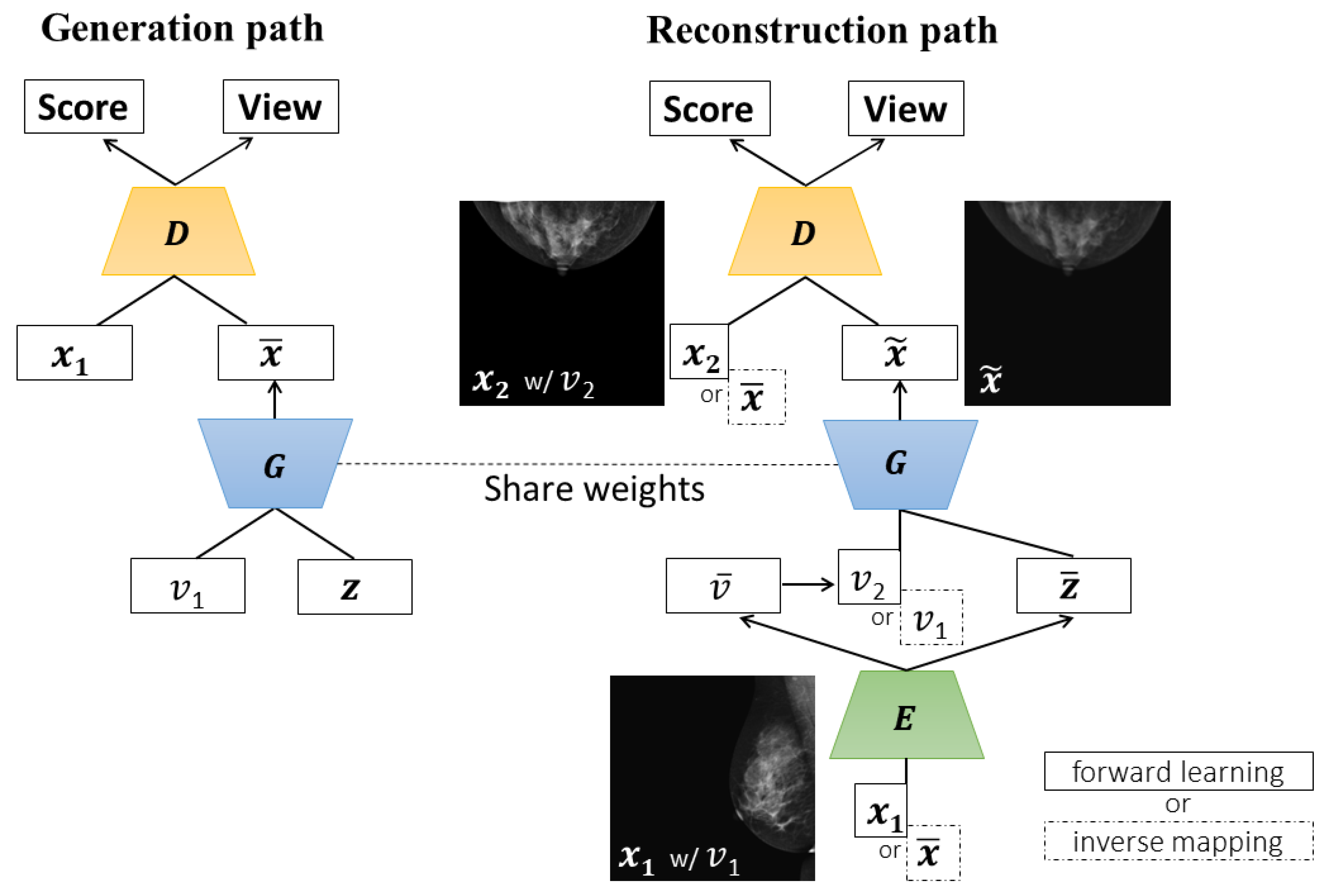
We adopted CR-GAN [32] as a fundamental image generation model to synthesize CC-view mammograms from MLO views. Furthermore, we aimed to generate higher resolution and superior quality mammograms through its combination with two approaches: A technique involving progressively increasing resolution [23] and feature matching loss [36]. First, we explain the CR-GAN framework specifically for our task. At the end of Section 2.1.1, we clarify our modified parts from the original CR-GAN. Then, we describe the incorporated approaches in Section 2.1.2 and Section 2.1.3.

2.1.1. CR-GAN

CR-GAN was developed to generate multi-view face images from single-view photographs using two-pathway networks [32]. The term complete representation suggests that the generation of superior-quality and identity-preserved images is guaranteed, even from unseen inputs not included in the training data set. The authors mentioned that the two-pathway networks enable coverage of the whole latent space and learning of complete representations. Conversely, an issue encountered by most GAN-based novel-view generation methods is that they learn only the training data and map only a subspace in the latent space, due to the single-pathway nature of the networks; namely, the encoder–decoder network used by the discriminator [28,29,30,31].

The two-pathway networks of CR-GAN include the generation and reconstruction paths. The two paths share the same generator (G). Figure 1 provides an illustration of the two-pathway networks used in our training. In the generation path, G takes random noise $\mathit{z}$ and a view label $v_1$, then tries to produce a realistic image $\overline{\mathit{x}}=G(v_1,\mathit{z})$. The label is a one-hot vector for MLO- or CC-view direction. The discriminator (D) is trained to distinguish $\overline{\mathit{x}}$ from a real image ${\mathit{x}}_{\mathbf{1}}$ labeled with $v_1$, by minimizing

$$\begin{array}{c}\hfill \underset{\mathit{z}\sim {\mathbb{P}}_{\mathit{z}}}{\mathbb{E}}\left[D_s\left(\overline{\mathit{x}}\right)\right]-\underset{\mathit{x}\sim {\mathbb{P}}_{\mathit{x}}}{\mathbb{E}}\left[D_s\left({\mathit{x}}_{\mathbf{1}}\right)\right]+{\lambda }_1\underset{\widehat{\mathit{x}}\sim {\mathbb{P}}_{\widehat{\mathit{x}}}}{\mathbb{E}}\left[\right(\left|\right|{\nabla }_{\widehat{\mathit{x}}}D\left(\widehat{\mathit{x}}\right){\left|\right|}_2-1{)}^2]-{\lambda }_2\underset{\mathit{x}\sim {\mathbb{P}}_{\mathit{x}}}{\mathbb{E}}\left[P(D_v\left({\mathit{x}}_{\mathbf{1}}\right)=v_1)\right],\end{array}$$

(1)

where ${\mathbb{P}}_x$ is a real data distribution, ${\mathbb{P}}_z$ is a noise uniform distribution, and ${\mathbb{P}}_{\widehat{x}}$ denotes arbitrary point of linear interpolation between the real distribution ${\mathbb{P}}_x$ and the generated distribution. Furthermore, $D_s(·)$ denotes the image quality, indicating how realistic the image is, $D_v(·)$ estimates the image view, and $P\left(D_v(·)\right)$ represents the probability of it being a specific view. G strives to fool D by maximizing

$$\begin{array}{c}\hfill \underset{\mathit{z}\sim {\mathbb{P}}_{\mathit{z}}}{\mathbb{E}}\left[D_s\left(\overline{\mathit{x}}\right)\right]+{\lambda }_3\underset{\mathit{z}\sim {\mathbb{P}}_{\mathit{z}}}{\mathbb{E}}\left[P(D_v\left(\overline{\mathit{x}}\right)=v_1)\right].\end{array}$$

(2)

The first and second terms in Equation (1) maximize the Wasserstein distance $\mathit{W}({\mathbb{P}}_r,{\mathbb{P}}_{\theta })$ between the probability distributions of the real and synthesized samples [22]:

$$\begin{array}{c}\hfill \mathit{W}({\mathbb{P}}_r,{\mathbb{P}}_{\theta })=\underset{\mathit{x}\sim {\mathbb{P}}_{\mathit{r}}}{\mathbb{E}}\left[D\left(\mathit{x}\right)\right]-\underset{\mathit{z}\sim {\mathbb{P}}_{\theta }}{\mathbb{E}}\left[D\left(\overline{\mathit{x}}\right)\right],\end{array}$$

(3)

where ${\mathbb{P}}_r$ is the real data distribution, ${\mathbb{P}}_{\theta }$ is the model distribution implicitly defined by $\overline{\mathit{x}}=G\left(\mathit{z}\right)$, and $\mathit{z}$ is sampled from a noise distribution. The third term in Equation (1) constrains the gradient norm of $D\left(\widehat{\mathit{x}}\right)$ with a penalty, because the optimized discriminator has an L2 norm of the gradient of almost 1, with respect to the input $\widehat{\mathit{x}}$, at any interpolation point.

The reconstruction path samples a real image pair $\mathit{x}$ = (${\mathit{x}}_1$, ${\mathit{x}}_2$), and aims to reconstruct ${\mathit{x}}_2$ from ${\mathit{x}}_1$. If ${\mathit{x}}_1$ is MLO-view, then ${\mathit{x}}_2$ is the CC-view of the identical subject, and vice versa. Although the purpose of this work is to synthesize CC views from MLO views, we conduct mainly bi-directional training and complementarily investigate unidirectional training. Incidentally, the original CR-GAN employs only bi-directional training. In bi-directional training, CC image syntheses from MLO views and MLO image syntheses from CC views are learned with equal probability (MLO⇔CC). On the other hand, in unidirectional training, only the production of CC views from MLO views (MLO⇒CC) is learned.

The encoder (E) and D are trained keeping G fixed. E receives ${\mathit{x}}_1$ and outputs a latent representation $\overline{\mathit{z}}$ with the estimated view $\overline{v}$, where ($\overline{v}$, $\overline{\mathit{z}}$) = ($E_v\left({\mathit{x}}_{\mathbf{1}}\right)$, $E_z\left({\mathit{x}}_{\mathbf{1}}\right)$). Hopefully, the outputs of E preserve the identity of the object, such that a complete representation is accomplished. For this purpose, CR-GAN utilizes inverse mapping that inputs the output from G back into the latent space, as proposed in BiGAN [38]; in other words, E is trained to be an inverse of G. For a 50/50 chance, ${\mathit{x}}_1$ is fed to E for realistic ${\mathit{x}}_2$ reconstruction (we refer to this as forward learning), or $\overline{\mathit{x}}$ is also fed for inverse mapping.

In the case of forward learning, G takes $\overline{z}=E_z\left({\mathit{x}}_{\mathbf{1}}\right)$ and $v_2$ as the input to produce $\tilde{\mathit{x}}$ = $G(v_2,\overline{z})$—a fake image of ${\mathit{x}}_{\mathbf{2}}$. D attempts to distinguish $\tilde{\mathit{x}}$ from the real ${\mathit{x}}_{\mathbf{2}}$ by minimizing

$$\begin{array}{c}\hfill \underset{{\mathit{x}}_{\mathbf{1}}\sim {\mathbb{P}}_{\mathit{x}}}{\mathbb{E}}\left[D_s\left(\tilde{\mathit{x}}\right)\right]-\underset{{\mathit{x}}_{\mathbf{2}}\sim {\mathbb{P}}_{\mathit{x}}}{\mathbb{E}}\left[D_s\left({\mathit{x}}_{\mathbf{2}}\right)\right]+{\lambda }_1\underset{\widehat{\mathit{x}}\sim {\mathbb{P}}_{\widehat{\mathit{x}}}}{\mathbb{E}}\left[\right(\left|\right|{\nabla }_{\widehat{\mathit{x}}}D\left(\widehat{\mathit{x}}\right){\left|\right|}_2-1{)}^2]-{\lambda }_2\underset{{\mathit{x}}_{\mathbf{2}}\sim {\mathbb{P}}_{\mathit{x}}}{\mathbb{E}}\left[P(D_v\left({\mathit{x}}_{\mathbf{2}}\right)=v_2)\right],\end{array}$$

(4)

where $\widehat{\mathit{x}}\sim {\mathbb{P}}_{\widehat{x}}$ is interpolated data from ${\mathit{x}}_{\mathbf{2}}$ and $\tilde{\mathit{x}}$. E lets G generate $\tilde{\mathit{x}}$ that resembles ${\mathit{x}}_{\mathbf{2}}$ by maximizing

$$\begin{array}{c}\hfill \underset{\mathit{x}\sim {\mathbb{P}}_{\mathit{x}}}{\mathbb{E}}[D_s\left(\tilde{\mathit{x}}\right)+{\lambda }_{3}P(D_v\left(\tilde{\mathit{x}}\right)=v_2)-{\lambda }_4{L}_1(\tilde{\mathit{x}},{\mathit{x}}_{\mathbf{2}})-{\lambda }_5{L}_v(E_v\left({\mathit{x}}_{\mathbf{1}}\right),v_1)],\end{array}$$

(5)

where $L_1$ is L1 regularization, used to bring $\tilde{\mathit{x}}$ as close as possible to ${\mathit{x}}_{\mathbf{2}}$. $L_v$, which is the cross-entropy loss of the view estimated by E and the true view, forces E to be a good view estimator. Equations (1), (2), (4), and (5) update the weights of the networks during forward learning.

For inverse mapping, G takes $\overline{\mathit{z}}$=$E_z\left(\overline{\mathit{x}}\right)$ and $v_1$ as the input, where $\overline{\mathit{x}}$ is derived from $v_1$ and random noise in the generator path. D is expected to distinguish $\tilde{\mathit{x}}$ = $G(v_1,E_z\left(\overline{\mathit{x}}\right))$ from the real image pair. Hence, $\widehat{\mathit{x}}$ in Equation (4) is modified to interpolated data from ${\mathit{x}}_{\mathbf{1}}$ and $\tilde{\mathit{x}}$. Equation (5) is also modified to

$$\begin{array}{c}\hfill \underset{\mathit{z}\sim {\mathbb{P}}_{\mathit{z}}}{\mathbb{E}}[D_s\left(\tilde{\mathit{x}}\right)+{\lambda }_{3}P(D_v\left(\tilde{\mathit{x}}\right)=v_1)-{\lambda }_4{L}_1(\tilde{\mathit{x}},\overline{\mathit{x}})]-{\lambda }_5\underset{{\mathit{x}}_{\mathbf{1}}\sim {\mathbb{P}}_{\mathit{x}}}{\mathbb{E}}\left[L_v(E_v\left(\overline{\mathit{x}}\right),v_1)\right],\end{array}$$

(6)

such that $\tilde{\mathit{x}}$ looks similar to $\overline{\mathit{x}}$. Equations (1), (2), (4), and (6) update the weights of the networks during inverse mapping.

While the original CR-GAN synthesizes 128 × 128 images, as can be determined from the code [34], we experimented with generating 256 × 256 and 512 × 512 images by adding convolution layers into the networks.

Table 1. Generator architecture of CR-GAN for 256 × 256 image synthesis.

	Type	Description of Type	Norm 1	Activation	Input Shape 2	Output Shape 2
Input projection	FC 3	Linear transformation	–	–	256	4 × 4 × 512
Layer 1	Convolution1	{Upsample→Conv2d(3,1,1)} +{BN→ReLU→Upsample →BN→ReLU→Conv2d(3,1,1)}			4 × 4 × 512	8 × 8 × 512
Layer 2					8 × 8 × 512	16 × 16 × 256
Layer 3					16 × 16 × 256	32 × 32 × 128
Layer 4					32 × 32 × 128	64 × 64 × 64
Layer 5					64 × 64 × 64	128 × 128 × 64
Layer 6			BN	ReLU	128 × 128 × 64	256 × 256 × 64
Layer 7	Convolution2	Conv2d(3,1,1)	–	Tanh	256 × 256 × 64	256 × 256 × 3

¹ Normalization. ² Width × height × channel. ³ Fully connected.

shows the architecture of G in the modified CR-GAN for 256 × 256 image syntheses. The second through sixth middle layers consist of Upsample (2× up-sampling by nearest neighbor method) and Conv2d (two-dimensional convolution; kernel size = 3, stride = 1, padding = 1). In each layer, the output feature vector from Conv2d after Upsample and that after passing repeatedly through batch normalization (BN), ReLU activation, Upsample, and Conv2d, in the order indicated by the right arrows (→), are summed. In the sixth layer, BN and ReLU are adapted again. Finally, the seventh layer translates the feature vector to a 256 × 256 image with 3 channels.

Table 2. Discriminator architecture of CR-GAN for 256 × 256 image synthesis.

	Type	Description of Type	Activation	Input Shape	Output Shape
Layer 1	Convolution1	Conv2d(3,1,1)	–	256 × 256 × 3	256 × 256 × 64
Layer 2	Convolution2	{Conv2d(3,1,1)→AvgPool2d} +{ReLU→Conv2d(3,1,1)→ReLU →Conv2d(3,1,1)→AvgPool2d}	ReLU	256 × 256 × 64	128 × 128 × 64
Layer 3				128 × 128 × 64	64 × 64 × 64
Layer 4				64 × 64 × 64	32 × 32 × 128
Layer 5				32 × 32 × 128	16 × 16 × 256
Layer 6				16 × 16 × 256	8 × 8 × 512
Layer 7				8 × 8 × 512	4 × 4 × 512
Layer 8-1	FC	Linear transformation	Softmax	4 × 4 × 512	2
Layer 8-2			–	4 × 4 × 512	1

shows the architecture of D. In the second through seventh layers, the feature vector after passing through Conv2d and AvgPool2d (two-dimensional average pooling; kernel size = 2), and that after passing through ReLU activation in addition to above the two functions repeatedly (in the order shown by the right arrows), are summed. In the eighth layer, the feature vector is fully connected, in order to output the estimated view information after proceeding with the Softmax function. In addition, the output from the seventh layer is translated to a scalar expressing the image quality, without the Softmax function. Batch normalization is not used in D. E has a similar architecture to D, but the eighth layer outputs the view information vector and image vector, with a shape of 256 × 256 × 3.

As a side note, Tian et al. have leveraged not only labeled images with view information, but also unlabeled images in self-supervised learning [32]. Meanwhile, the view information of mammograms is usually obvious, and this information can be easily extracted from the images. Therefore, we used only labeled mammograms without self-supervised learning.

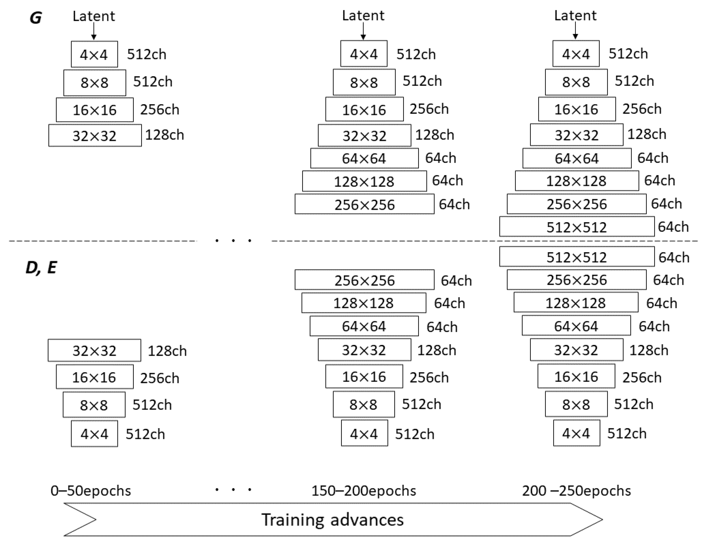
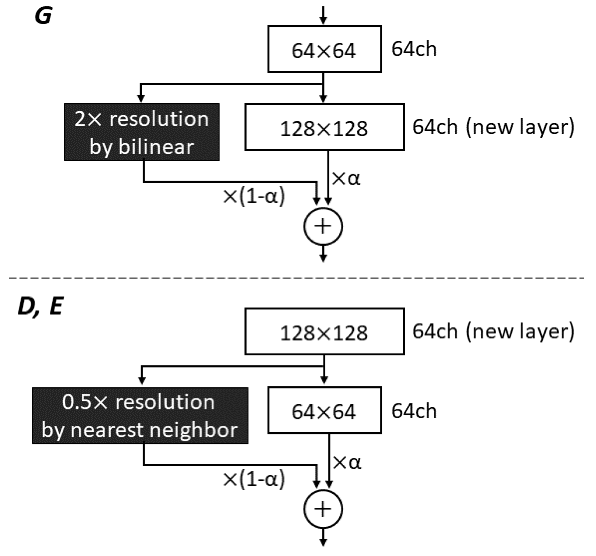
2.1.2. Progressive Growing Technique

We incorporated a technique for gradually increasing the image resolution in the networks, as proposed for PG-GAN by Karras et al. [23]. They started training with 4 × 4 low-resolution images, and added new layers to progressively increase the resolution in both G and D. This approach permits the networks to first obtain large-scale image features, followed by directing attention to increasingly finer scale features. The authors also used WGAN-GP loss as one of the loss functions. Eventually, PG-GAN was used to produce 1024 × 1024 images with convincing realism. The progressive growing (PG) technique can offer more stable and faster training, compared with simultaneously learning all scales. Utilizing this technique for not only G and D, but also E in CR-GAN, we attempted to increase the generated image resolution to 512 × 512 starting from 32 × 32, as shown in Figure 2. We added a new layer to each network per 50 training epochs, in order to increase the generated image resolution. When inserting the new layer into G, we doubled the resolution of the previous layer using bilinear interpolation, thus matching the resolution of the new layer. Next, the up-sampled feature vector from the last layer and the vector from the new layer were summed with weights (1-$\alpha$) and $\alpha$, respectively, where $\alpha$ increases linearly from 0 to 1 each 50 epochs as the training progresses (see Figure 3). Similarly, when an image with doubled resolution is newly fed into D and E, the feature vector from the new layer is down-scaled using the nearest neighbor method, in order to ensure that the same resolution is preserved between layers. The down-scaled vector and the vector from the next layer are also combined through weighted summation. In the original work on PG-GAN, the resolution was transited in the three channels of RGB colors [23]; however, except in the case of 32 × 32 resolution with 128 channels, we operate the resolution transition in 64 channels, in order to reduce the load on the GPU by making the network layers as shallow as possible.

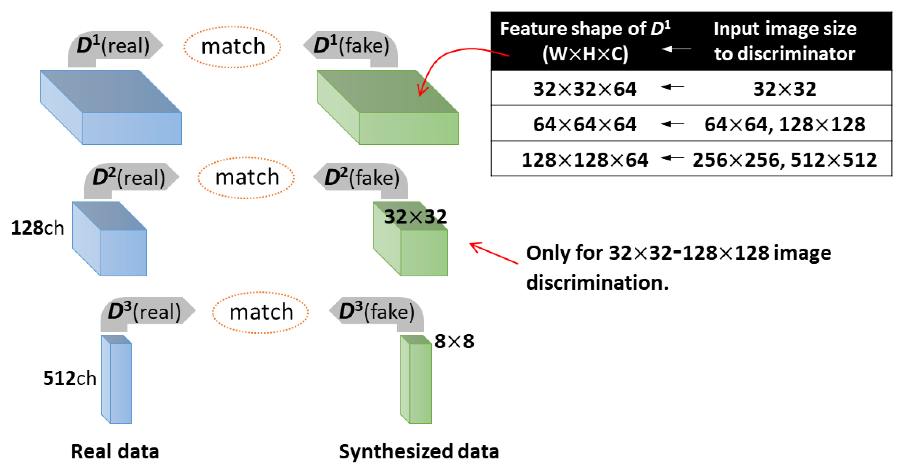
2.1.3. Feature Matching Loss

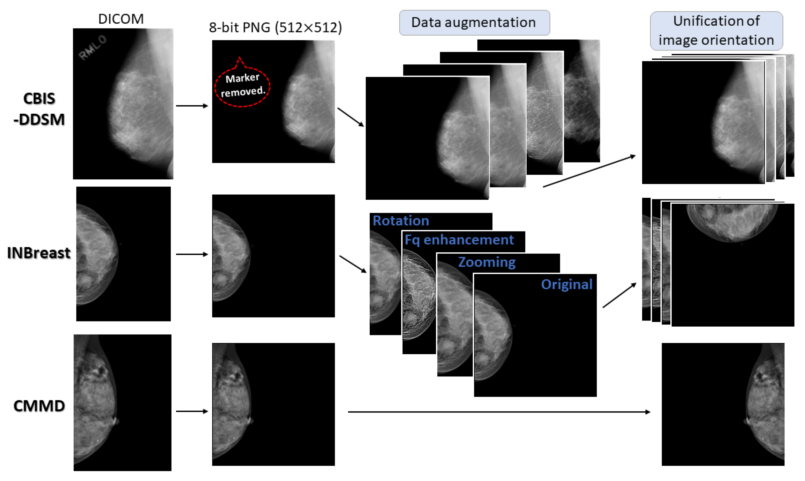
We introduced feature matching loss as an additional loss function into CR-GAN, and examined its effects. Based on a similar idea to perceptual loss [37], feature matching loss ($L_{FM}$) has been proposed by Wang et al. [36] for synthesizing high-resolution images with 1024 × 1024 matrices. $L_{FM}$ is calculated by L1 regularization from feature vectors in multiple layers of D, using constraints to match intermediate representations between real and synthesized images. Introducing $L_{FM}$ in the generator loss, D works as a multi-scale discriminator. Wang et al. remarked that this loss stabilizes training and drives D to produce more natural images. In the case of forward learning, $L_{FM}$ is calculated as follows:

$$\begin{array}{c}\hfill L_{FM}=\underset{\mathit{x}\sim {\mathbb{P}}_{\mathit{x}}}{\mathbb{E}}\frac{1}{N}\sum _{i=1}^N\left[\right||D^i\left(G({\mathit{v}}_{\mathbf{2}},\overline{\mathit{z}})\right)-D^i\left({\mathit{x}}_{\mathbf{2}}\right){\left|\right|}_1],\end{array}$$

(7)

where N is the total number of the layers used for the loss calculation, and $D^i$ denotes the extracted feature vector in each layer of D. In the case of inverse mapping,

$$\begin{array}{c}\hfill L_{FM}=\underset{\mathit{z}\sim {\mathbb{P}}_{\mathit{z}}}{\mathbb{E}}\frac{1}{N}\sum _{i=1}^N\left[\right||D^i\left(G({\mathit{v}}_{\mathbf{1}},\overline{\mathit{z}})\right)-D^i\left(\overline{\mathit{x}}\right){\left|\right|}_1].\end{array}$$

(8)

When the image input into the discriminator has a resolution ranging from 32 × 32 to 128 × 128, we set N to 3, and $D^i$ was extracted from the three middle layers. The shape of $D^1$ depends on the input image size to D, as illustrated in Figure 4. $D^2$ and $D^3$ are the feature vectors with 32 × 32 × 128 and 8 × 8 × 512 shapes, respectively. When a 256 × 256 or 512 × 512 image is fed into D, we change N to 2 to reduce the training time and GPU load. Accordingly, $L_{FM}$ is calculated using two vectors with shape 128 × 128 × 64 and 8 × 8 × 512, respectively. We investigated whether the image quality is improved by adding $L_{FM}$ to Equation (5) or (6).

2.2. Data Sets

We used image data from the following publicly available mammogram databases: Curated Breast Imaging Subset of Digital Database for Screening Mammography (CBIS-DDSM) [39], INBreast database [40], and the Chinese Mammography Database (CMMD) [41]. The images in CBIS-DDSM are 16-bit digital data scanned from analog film mammograms in the Digital Imaging and Communications in Medicine (DICOM) format. The matrix sizes vary within the range from approximately 3000 × 4500 to 4000 × 5700. The INBreast database was acquired using a direct-conversion flat panel detector system (Siemens Mammomat Novation DR). The images are 3328 × 4084 or 2560 × 3328 matrices, depending on the used compression plate sizes. The images were saved in DICOM format with a 14-bit contrast resolution. The CMMD database was acquired using an indirect-conversion flat panel detector system (GE Senographe DS). The images were saved in DICOM format with 8-bit contrast resolution as 1914 × 2294 matrices. We excluded cases from the databases if they contained critical positioning errors, large artifacts (e.g., film scratches, dust particles), and foreign bodies (e.g., biopsy clip markers, pacemakers, implants). Eventually, we chose 1054 two-view mammograms (MLO- and CC-view pairs) from CBIS-DDSM, 188 pairs from INBreast, and 2542 pairs from CMMD. The right and left two-view mammograms of identical subjects were individually counted. From each database, 80% of pairs were used for training, while the remaining 20% of pairs were used for testing. We ensured that the mammograms of identical subjects were not divided into the training and test data sets, in order to avoid train–test contamination.

2.3. Pre-Processing for Training

The DICOM data from the above three databases were converted into 8-bit portable network graphics (PNG) format images. All the image sizes were reduced to 512 × 512 by bilinear interpolation. We replaced tiny artifacts, such as dust particles, with the surrounding pixels. As most CBIS-DDSM images include X-ray markers indicating anatomical sides and view directions (e.g., “R-MLO”), the image pixels on the markers were replaced with a pixel value of 0. Figure 5 depicts the pre-processing flow.

Moreover, we applied data augmentation to the images from CBIS-DDSM and INBreast using image zooming (in or out), high-frequency enhancements, contrast and brightness adjustments, image rotations, and image shifts. Every augmentation was carried out within realistic mammographic conditions, such as image rotation angles within 5 degrees. Image zooming was forced, for each MLO mammogram, to include entire breast tissue and pectoralis major muscle and, for each CC mammogram, to include entire breast tissue. The same augmentation processing was adapted to MLO and CC paired mammograms of respective subjects. In some cases, multiple image processing was combined on the paired mammograms. Consequently, the number of training image pairs from CBIS-DDSM and INBreast was increased by fourfold.

In addition, the left-MLO mammograms were horizontally flipped, such that MLO-image orientations were unified regardless of the anatomical breast side. The right CC mammograms were rotated 90 degrees to the right, and the left CC mammograms were rotated 90 degrees to the left. The image orientations of the CC and MLO-view mammograms thereafter became similar to those of frontal and side-face photographs, respectively.

2.4. Experimental Environment and Parameter Settings

We used an NVIDIA GeForce RTX 3080 Ti with 16 GB GPU memory for training. The training and testing were conducted using a Pytorch 1.11.0 framework and Jupyter Notebook on the Windows 10 operating system. During training, the Adam optimizer was used, with a learning rate of 0.0001 and the following momentum parameters: ${\beta }_1$ = 0 and ${\beta }_2$ = 0.9. We employed batch sizes of 10 and 4 for 256 × 256 image synthesis. In contrast, we fixed it at 20 for 128 × 128 and 4 for 512 × 512 image syntheses. Inevitably, 20, 10, and 4 were the respective highest batch sizes not inducing the system to be out of memory on the GPU for 128 × 128, 256 × 256, and 512 × 512 image syntheses. The maximum epochs were set as 155, 205, and 255 for the 128 × 128, 256 × 256, and 512 × 512 image syntheses, respectively. In fact, under the PG technique adaptation, an additional five epochs of training were conducted after $\alpha$ reached 1 in the final resolution syntheses. We set ${\lambda }_1$ = 10, ${\lambda }_2\sim {\lambda }_4$ = 1, and ${\lambda }_5$ = 0.01, as in the original CR-GAN [32].

2.5. Performance Evaluation

We evaluated the performance of CR-GAN and our proposed models in terms of the image similarity of each pair between the real and synthesized images. The Frèchet inception distance (FID) has been widely used for performance analyses of GAN models [42,43]. Karras et al. have used the sliced Wasserstein distance (SWD) to assess the performance of PG-GAN [23]. Nonetheless, these metrics measure distances between synthetic and real data distributions; that is, the FID and SWD evaluate not the similarity between each real and fake sample, but the entire similarity between the two groups. Thereby, we used the peak signal to noise ratio (PSNR), structural similarity (SSIM) [44], multi-scale SSIM (MS-SSIM) [45], and cosine similarity (Cos_sim) to evaluate the similarity between pairs of real and synthesized CC-view mammograms for the test data set described in Section 2.2.

The PSNR measures the image similarity based on the ratio of noise to the maximum pixel value, as follows:

$$\begin{array}{c}\hfill PSNR=10{log}_{10}\left(\frac{P_{max}}{MSE}\right),\end{array}$$

(9)

where MSE is the mean square error (MSE) between two images, and $P_{max}$ is the maximum value of the image pixels. If the images have 8-bit contrast resolution, $P_{max}$ is 255. The higher the PSNR value, the more similar the two images.

SSIM computes the image similarity between two images ($\mathbf{x}$,$\mathbf{y}$) using the three components of brightness, contrast, and structure, as shown in Equation (10):

$$\begin{array}{c}\hfill SSIM(\mathbf{x},\mathbf{y})=\left[l\right(\mathbf{x},\mathbf{y}\left)\right]\left[c\right(\mathbf{x},\mathbf{y}\left)\right]\left[s\right(\mathbf{x},\mathbf{y}\left)\right],\end{array}$$

(10)

where $l(\mathbf{x},\mathbf{y})$ is the brightness comparison, $c(\mathbf{x},\mathbf{y})$ is the contrast comparison, and $s(\mathbf{x},\mathbf{y})$ is the structural comparison [44]. The respective components are calculated according to the means, variances, and covariances of $\mathbf{x}$ and $\mathbf{y}$. The SSIM value ranges between 0 and 1; as the similarity increases, the value becomes closer to 1.

MS-SSIM has been introduced as an alternative metric of SSIM, incorporating image details at various resolutions [45]. MS-SSIM is calculated by combining the three components of SSIM on multiple scales, as follows:

$$\begin{array}{c}\hfill SSIM(\mathbf{x},\mathbf{y})={\left[l_M(\mathbf{x},\mathbf{y})\right]}^{{\alpha }_M}·\prod _{j=1}^M{\left[c_j(\mathbf{x},\mathbf{y})\right]}^{{\beta }_j}{\left[s_j(\mathbf{x},\mathbf{y})\right]}^{{\gamma }_j}.\end{array}$$

(11)

The two images ($\mathbf{x}$,$\mathbf{y}$) are iteratively low-pass filtered and down-sampled by a factor of 2. The scale of the original image is 1, while that of the most reduced image is M. The brightness comparison is computed only at scale M, and we refer to this as $l_M(\mathbf{x},\mathbf{y})$. The contrast and structure comparison components are calculated at each scale, denoted as $c_j(\mathbf{x},\mathbf{y})$ and $s_j(\mathbf{x},\mathbf{y})$ for the $j^{\mathrm{th}}$ scale, respectively. Wang et al. [45] have obtained five-scale parameters, in which the SSIM scores agreed with subjective assessments. The resulting parameters were ${\beta }_1$ = ${\gamma }_1$ = 0.0448, ${\beta }_2$ = ${\gamma }_2$ = 0.2856, ${\beta }_3$ = ${\gamma }_3$ = 0.3001, ${\beta }_4$ = ${\gamma }_4$ = 0.2363, and ${\alpha }_5$ = ${\beta }_5$ = ${\gamma }_5$ = 0.1333. We also used these parameters in our performance evaluation.

Cos_sim is commonly used to determine the similarity between two vectors [46]. In some self-supervised contrastive learning methods (which have developed rapidly in recent years), Cos_sim has been utilized in classification tasks by placing similar images closer and dissimilar images further from each other in the latent space [46,47]. Cos_sim is defined in terms of the cosine of the angle between the two vectors, and is calculated as follows:

$$\begin{array}{c}\hfill Cos\_sim(\mathbf{x},\mathbf{y})=\frac{\mathbf{x}·\mathbf{y}}{\left|\right|\mathbf{x}\left|\right|\left|\right|\mathbf{y}\left|\right|}.\end{array}$$

(12)

Cos_sim takes values within the interval from −1 to 1. When two images are more similar, the Cos_sim value is closer to 1.

3. Results

3.1. Comparison of the Similarity Metrics by Training Methods

The similarity metrics were calculated and compared between the real and synthesized CC-view mammograms for the test data set.

Table 3. Image similarity metrics and training time with respect to the training settings.

Resolution	Batch Size	Model	Training Direction	PSNR	SSIM	MS-SSIM	Cos_sim	Time (h)
128 × 128	20	CR-GAN	Bi-directional	21.9	0.746	0.842	0.817	16.8
		CR-GAN+PG		23.0	0.742	0.858	0.877	21.8
		CR-GAN+PG$+L_{FM}$		23.9	0.754	0.883	0.889	23.0
		CR-GAN+PG$+L_{FM}$	Unidirectional	22.0	0.705	0.838	0.829	10.6
256 × 256	10	CR-GAN	Bi-directional	21.3	0.727	0.812	0.845	87.9
		CR-GAN+PG		20.2	0.736	0.827	0.871	36.4
		CR-GAN+PG$+L_{FM}$		23.9	0.767	0.857	0.890	38.2
		CR-GAN+PG$+L_{FM}$	Unidirectional	21.2	0.730	0.821	0.799	30.1
	4	CR-GAN	Bi-directional	NA 1	NA	NA	NA	NA
		CR-GAN+PG
		CR-GAN+PG$+L_{FM}$		23.1	0.766	0.852	0.876	72.8
512 × 512	4	CR-GAN+PG	Bi-directional	NA	NA	NA	NA	NA
		CR-GAN+PG$+L_{FM}$		22.7	0.766	0.831	0.868	112.4
		CR-GAN+PG$+L_{FM}$	Unidirectional	NA	NA	NA	NA	NA

¹ Not available.

lists the averaged metrics and the required training time, with respect to the training settings. The highest metrics in each image resolution setting are in bold.

We attempted to synthesize 256 × 256 images with the method using only CR-GAN or the model incorporating the PG technique with batch of 4 in the bi-directional training. However, blank images with all pixel values set to a constant were generated, due to the discriminator losses in Equations (1) and (4) and the generator losses in Equations (2) and (5) diverging. Moreover, we also attempted to synthesize 512 × 512 images using bi-directional training with the PG technique and the unidirectional training with both the PG technique and $L_{FM}$. Nevertheless, these two methods also failed due to divergence of the loss functions. These results are listed as NA (not available) in Table 3. In addition, training using only CR-GAN for 512 × 512 image syntheses took longer than a week, so we did not conduct training, in order to prevent the GPU from being subjected to such a long-term and high-heat load. Consequently, we investigated only bi-directional training with both the PG technique and $L_{FM}$ as the only feasible method of those for synthesizing 512 × 512 images.

When synthesizing 128 × 128 images through bi-directional training, there was a slight increase in the three similarity metrics (PSNR, MS-SSIM, and Cos_sim; p < 0.05) for the model incorporating the PG technique, compared with the method using only CR-GAN, as shown in Table 3. However, the method with PG required 21.8 h of training time; longer than the 16.8 h when using only CR-GAN. Next, there were statistically significant increases in all evaluated similarity metrics (p < 0.05) when using the model incorporating both the PG technique and $L_{FM}$, compared with the model using only CR-GAN, although the training time was further extended. In the case of 256 × 256 image synthesis, the model incorporating the PG technique notably reduces the training time to 36.4 h, compared with 87.9 h for the model using only CR-GAN. With regard to the similarity metrics, significant increases (p < 0.05) in SSIM, MS-SSIM, and Cos_sim are obtained with the method incorporating PG technique, compared to the method using only CR-GAN. When $L_{FM}$ was also adapted to CR-GAN with the PG technique, all similarity metrics further significantly increased (p < 0.05), while the bi-directional training time was only extended by a few hours.

Table 3 also compares the performance between bi-directional (MLO⇔CC) and unidirectional (MLO⇒CC) training when incorporating the PG technique and $L_{FM}$. In both cases at 128 × 128 and 256 × 256 resolutions, the metrics indicated higher image similarity for bi-directional training, with statistically significant differences (p < 0.05), compared with unidirectional training, which had the advantage of shorter training time. In summary, CR-GAN incorporating both the PG technique and $L_{FM}$ in bi-directional training led to the highest values for the similarity metrics.

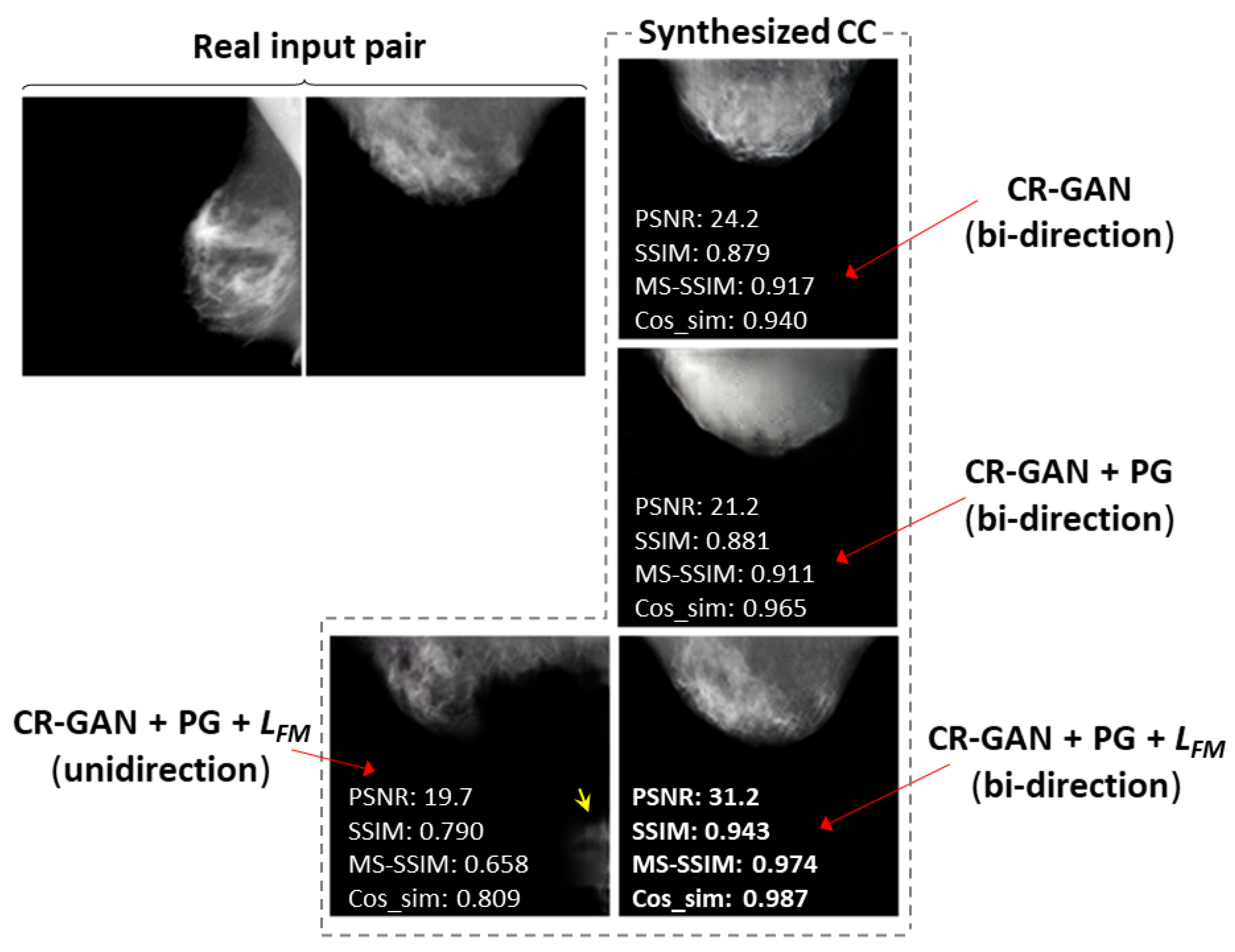
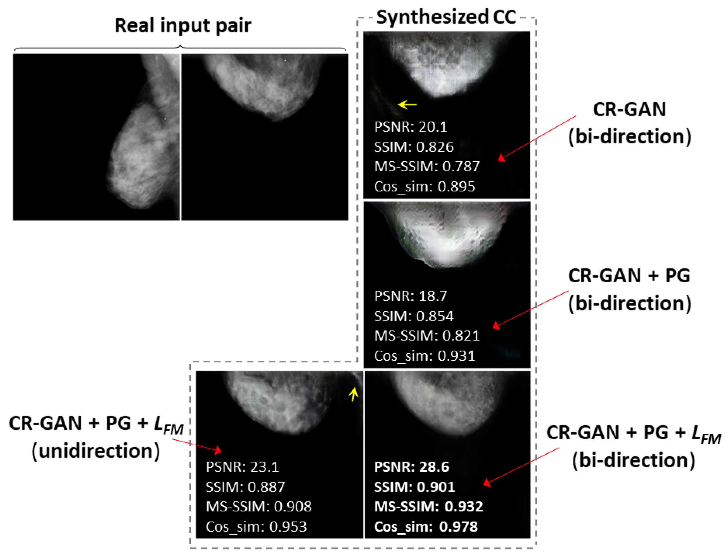
3.2. Comparison of Images Synthesized by Different Training Methods

As an example of a successful case, we selected the case of bi-directional training with the PG technique and $L_{FM}$, which achieved the synthesis of CC views that were visually similar to the real CC views at 128 × 128 resolution. Figure 6 compares the synthesized images and the similarity metrics for each training method in the successful case. We also selected another successful case at 256 × 256 resolution, and compared the synthesized images and similarity metrics for the training methods, as shown in Figure 7. In most cases, including Figure 6 and Figure 7, we observed CC views that were the most realistic and visually similar to real views when synthesized using the bi-directional method with PG technique and $L_{FM}$. The values of the similarity metrics were higher than those obtained for other training methods. In the images synthesized by the method using only CR-GAN, we can see obvious differences from the real views, in terms of the mammary gland shapes or textures. The sharpness was noticeably deteriorated in the images synthesized by the method using the PG technique without $L_{FM}$, although the similarity metrics tended to be slightly increased, compared to the results of the method using only CR-GAN, as shown in Table 3. Additionally, there were artifacts at locations outside the breast in some views synthesized by the method using only CR-GAN or unidirectional training, as indicated by yellow arrows in Figure 6 and Figure 7.

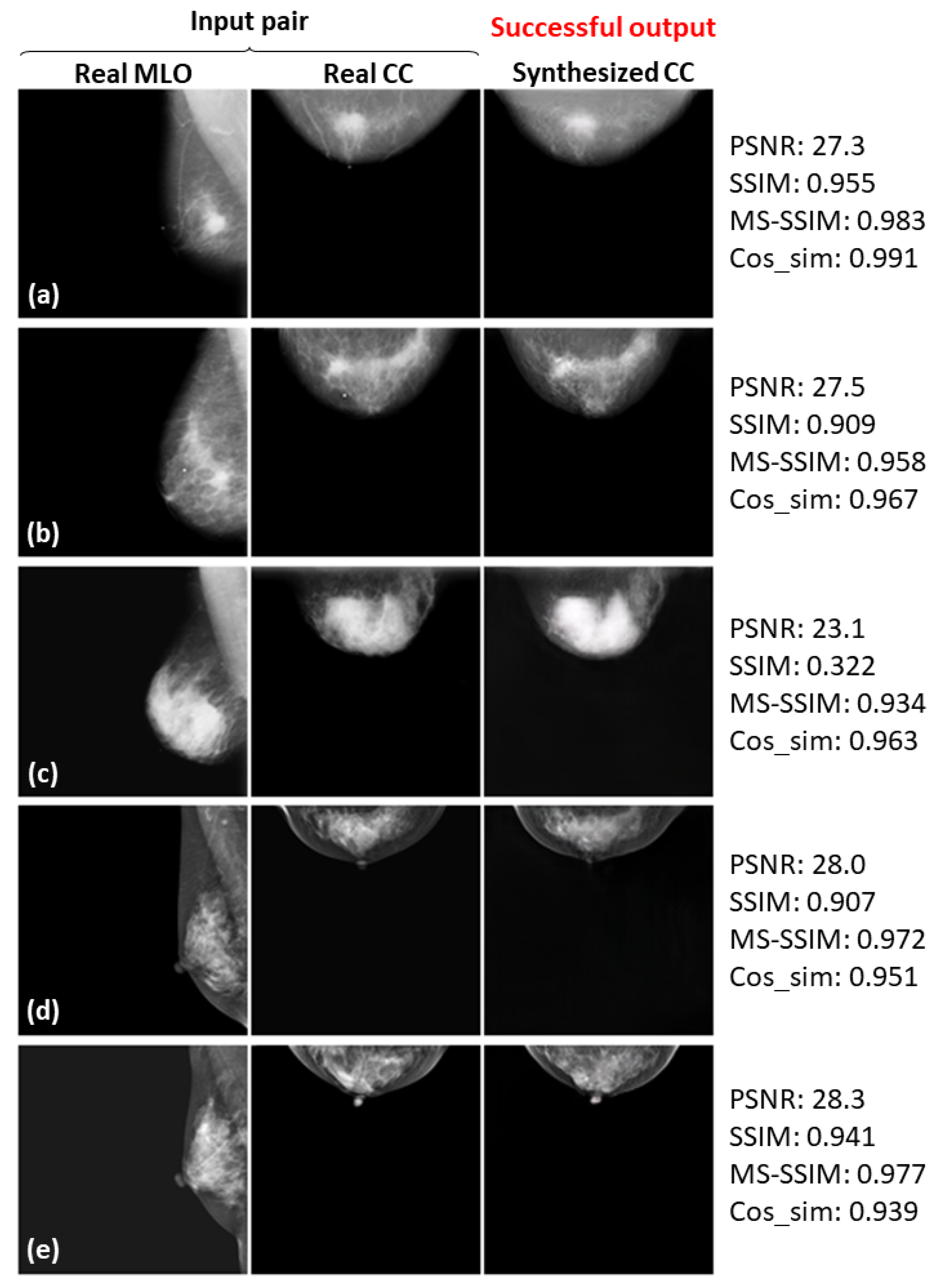
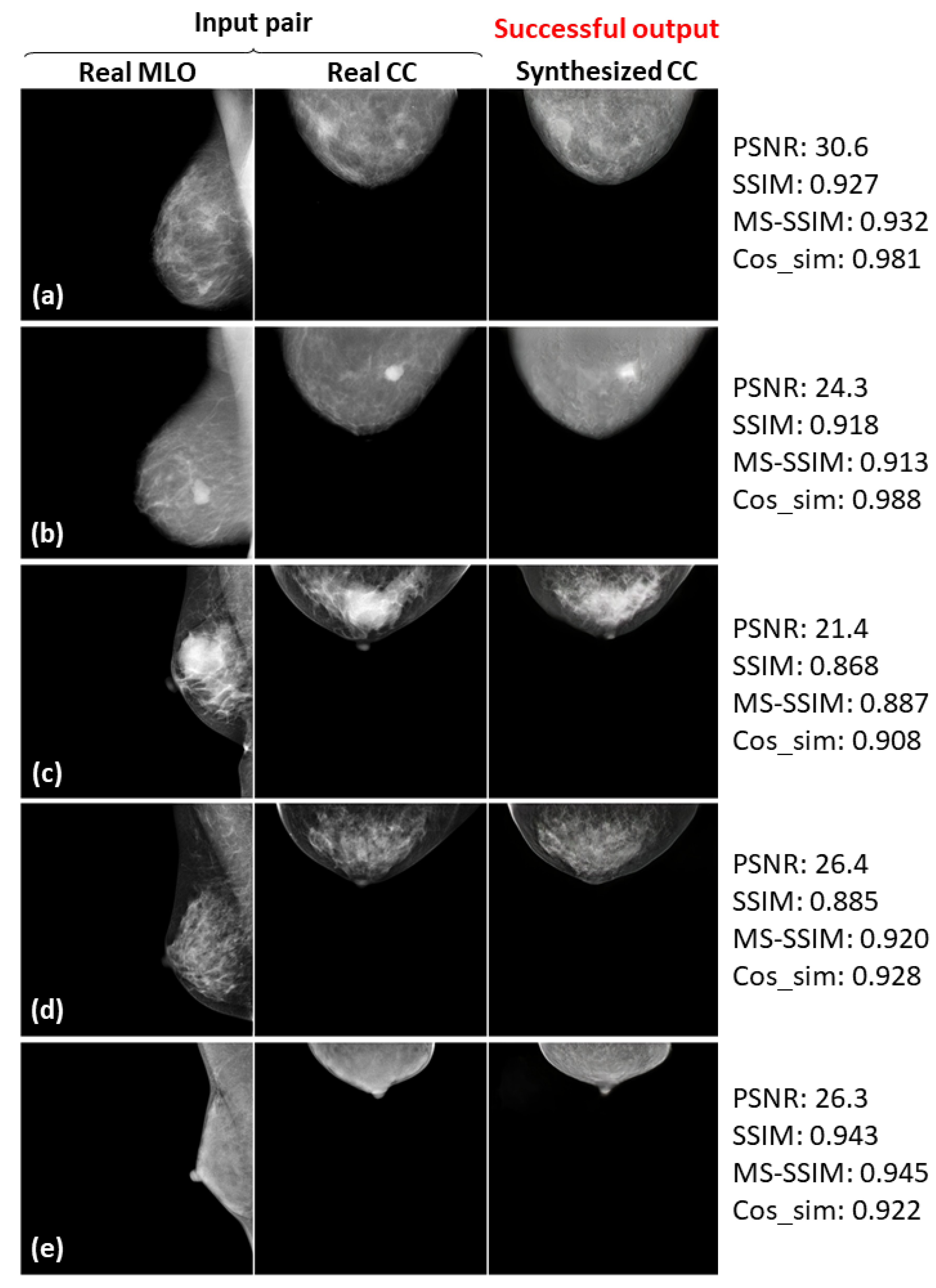
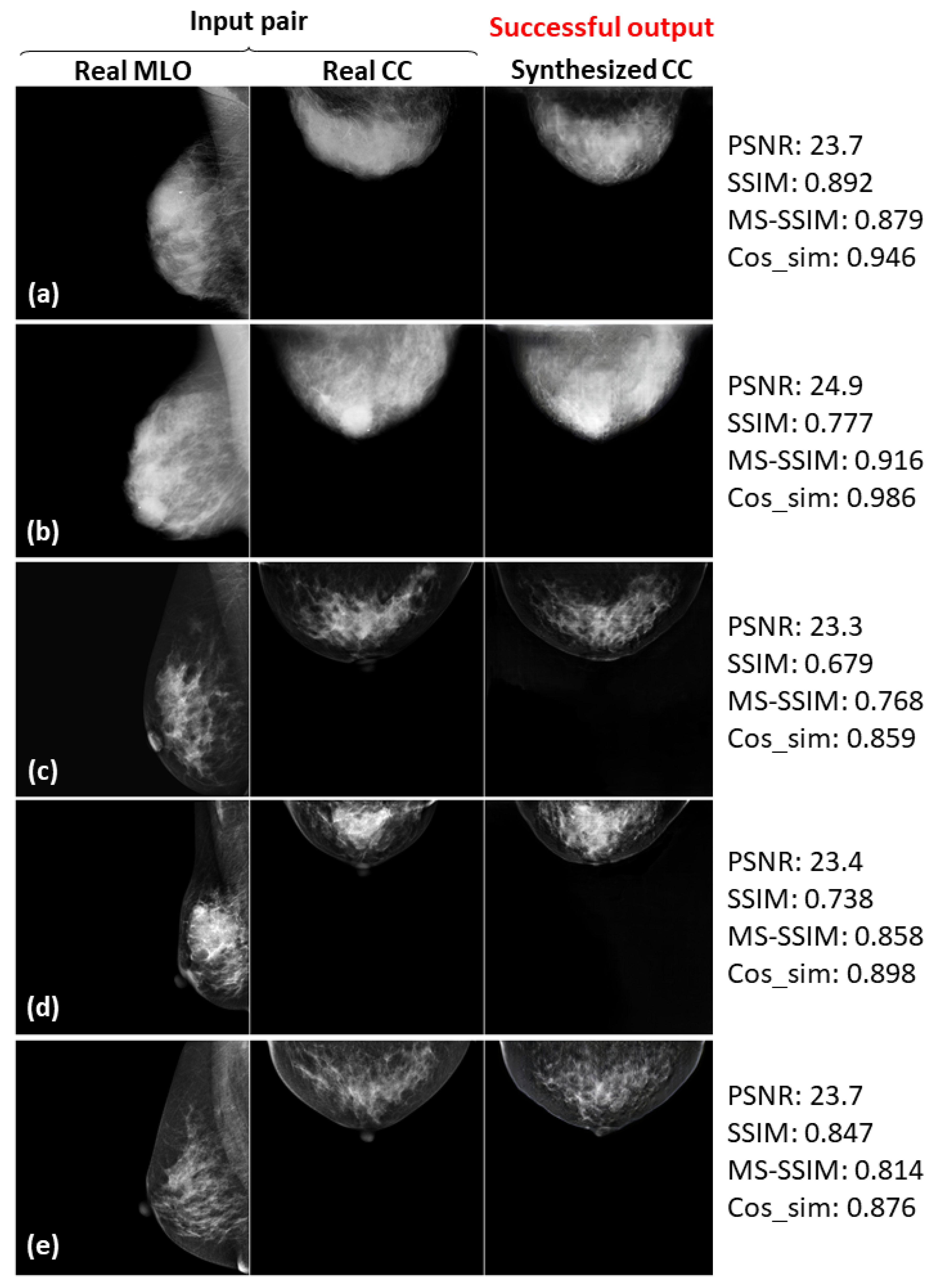
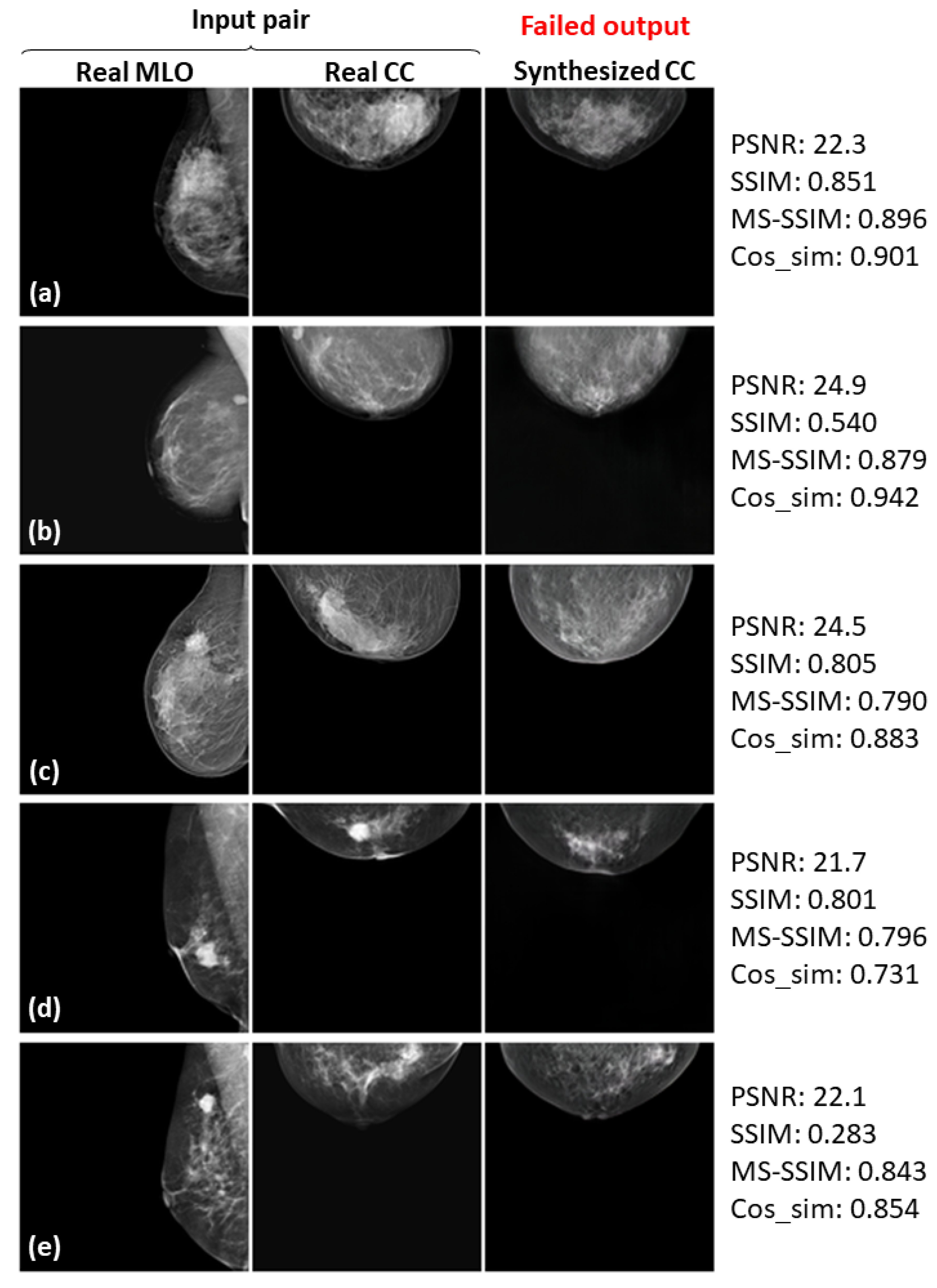
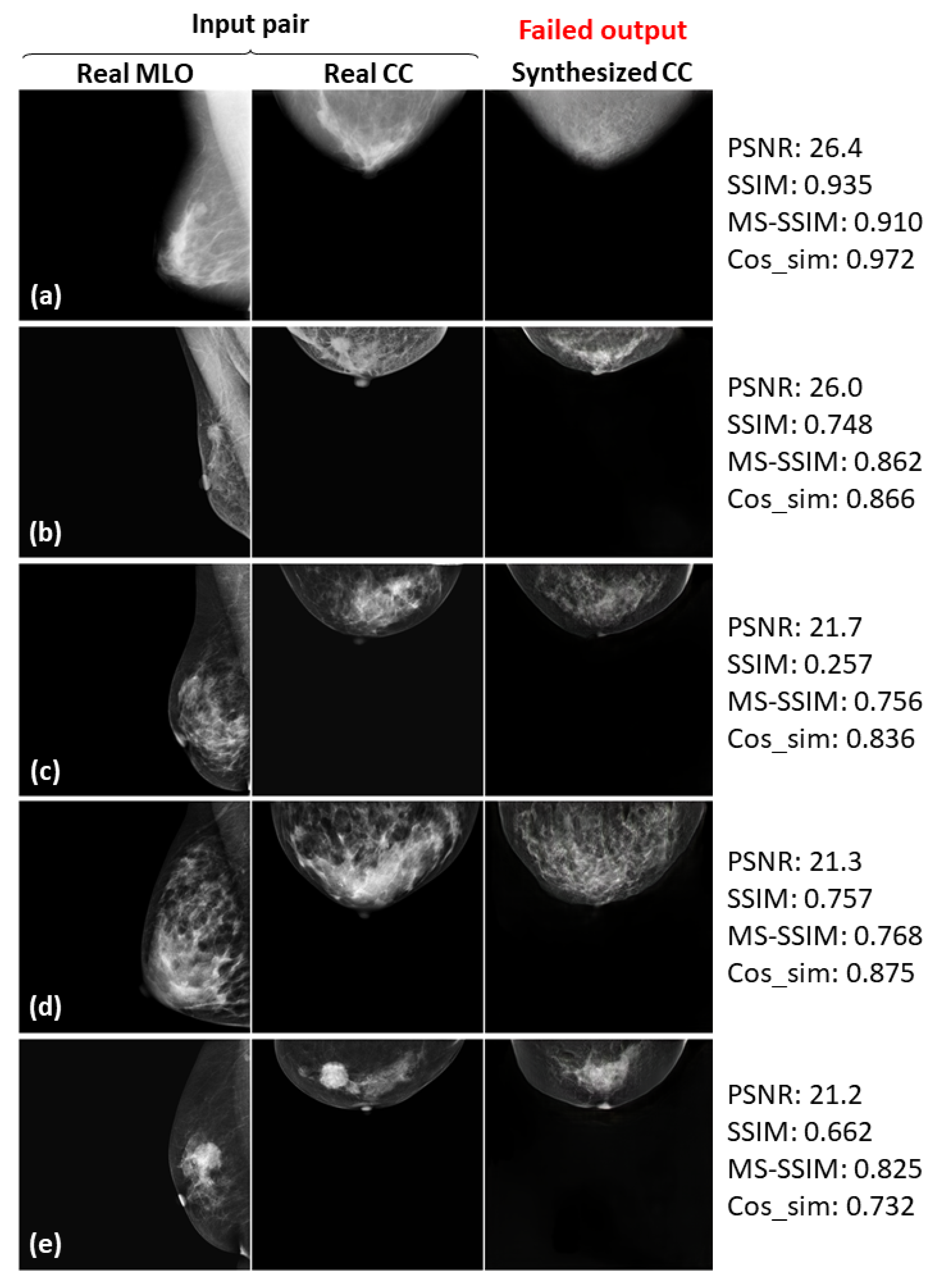
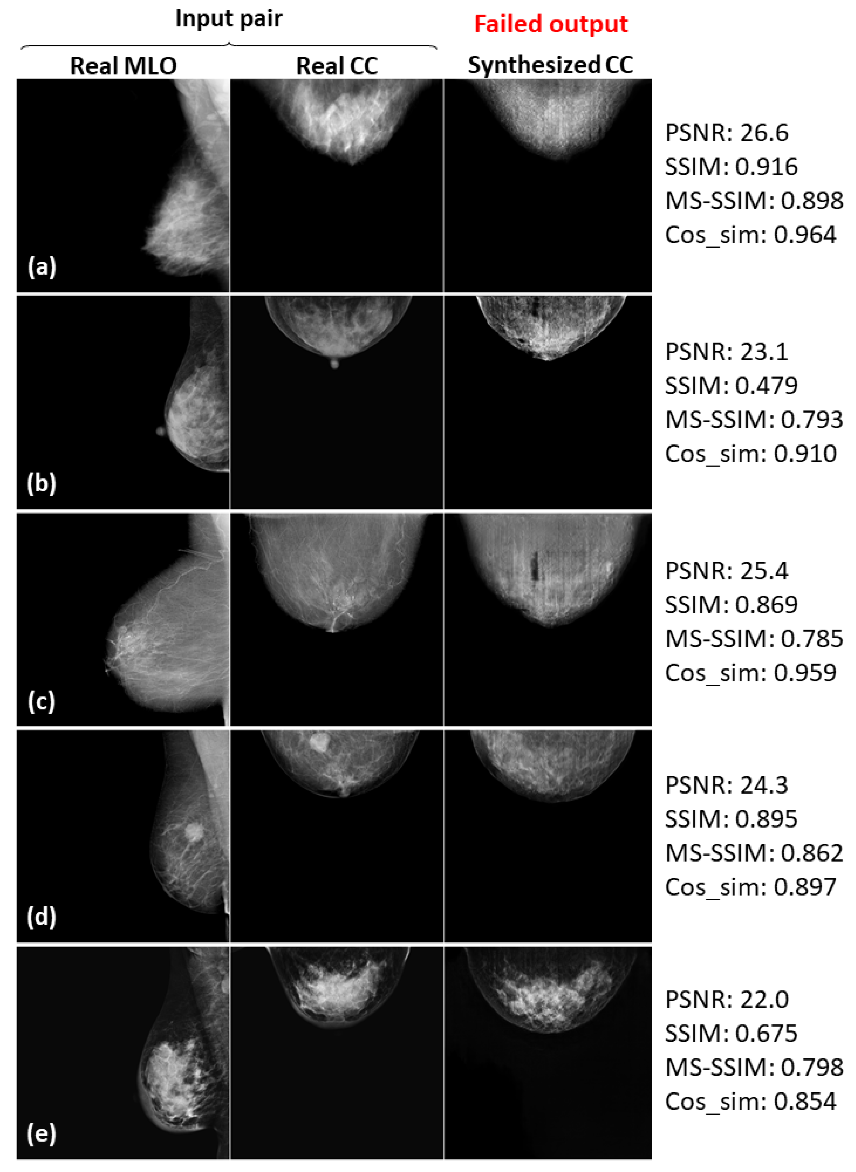
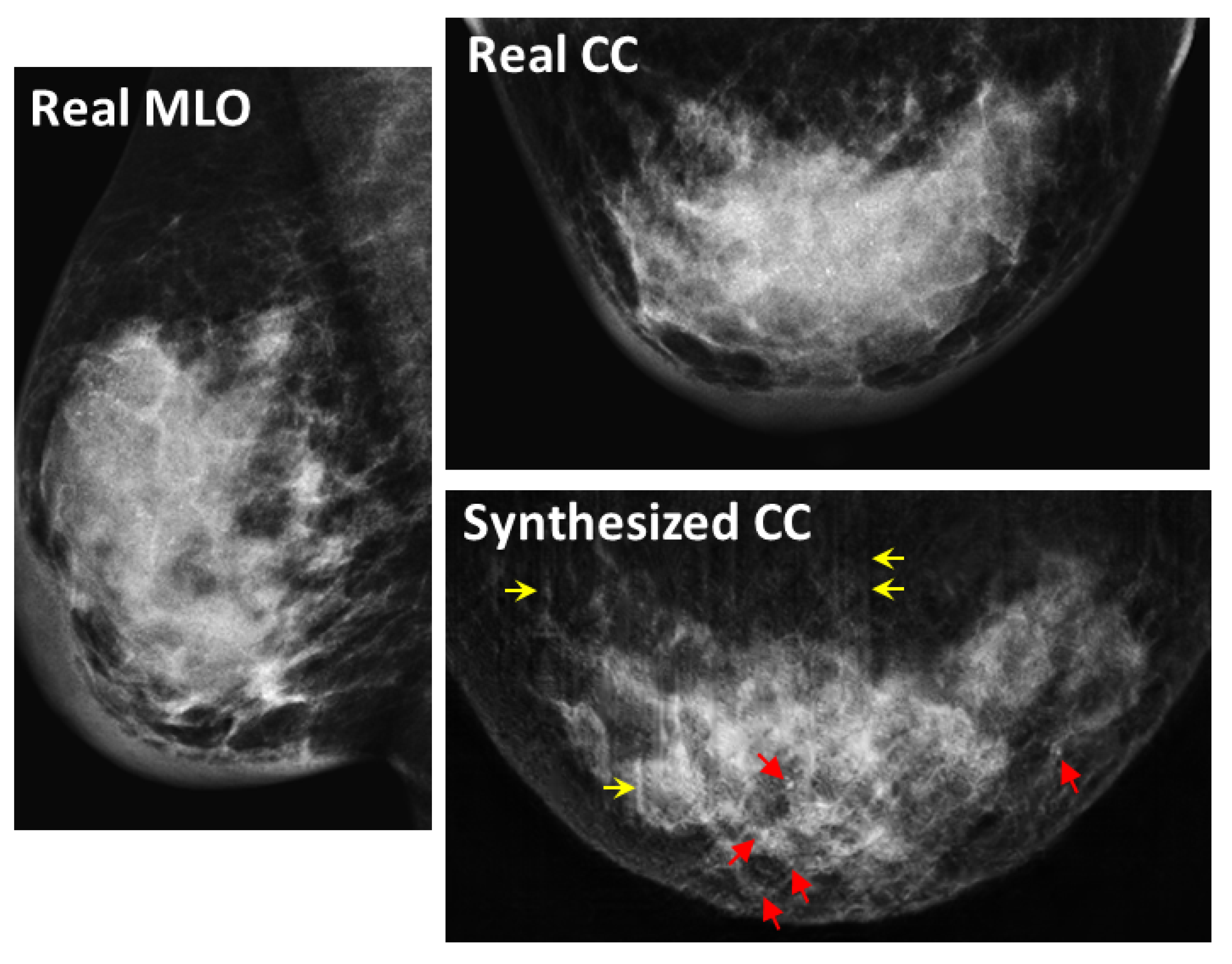
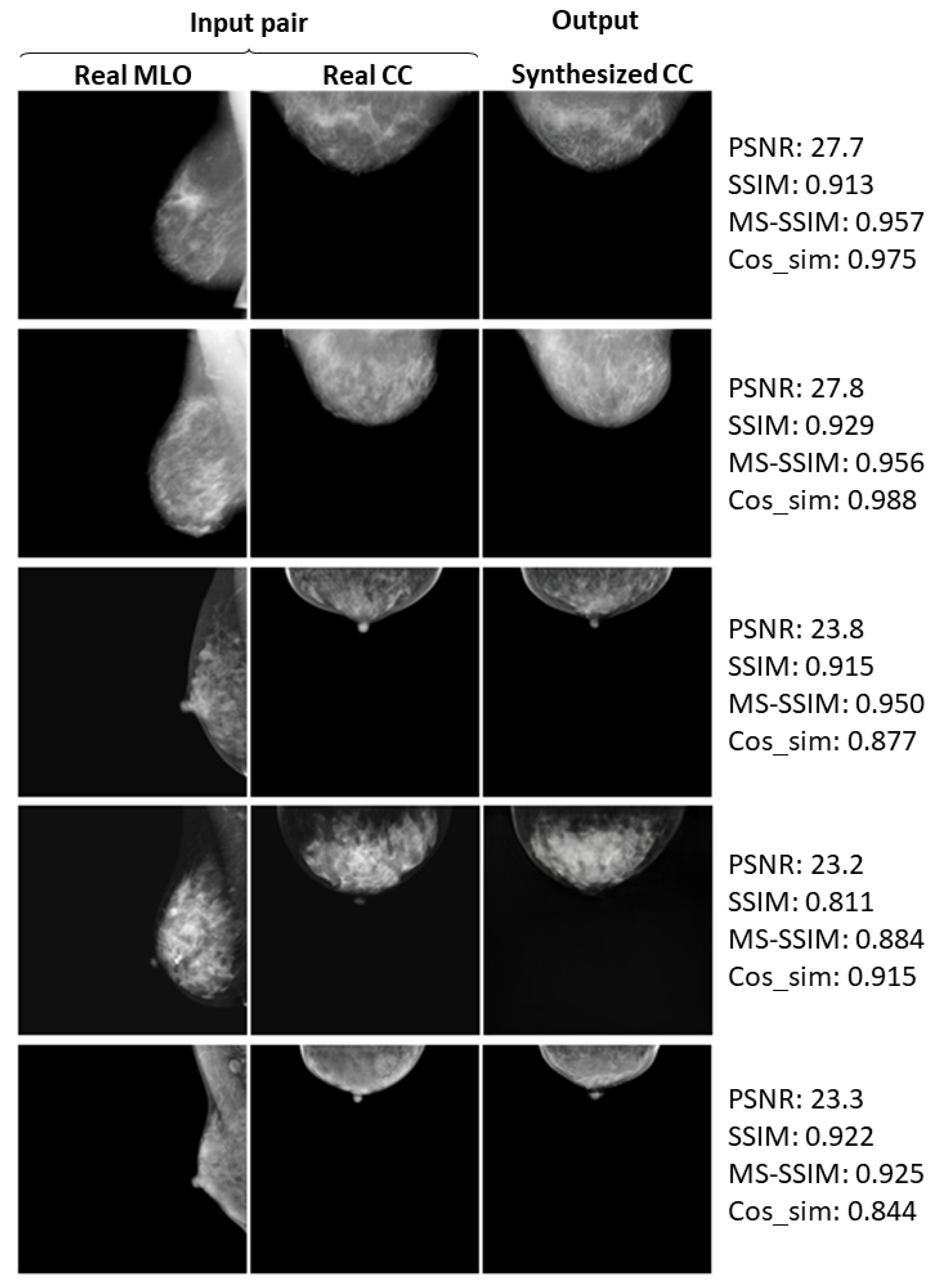
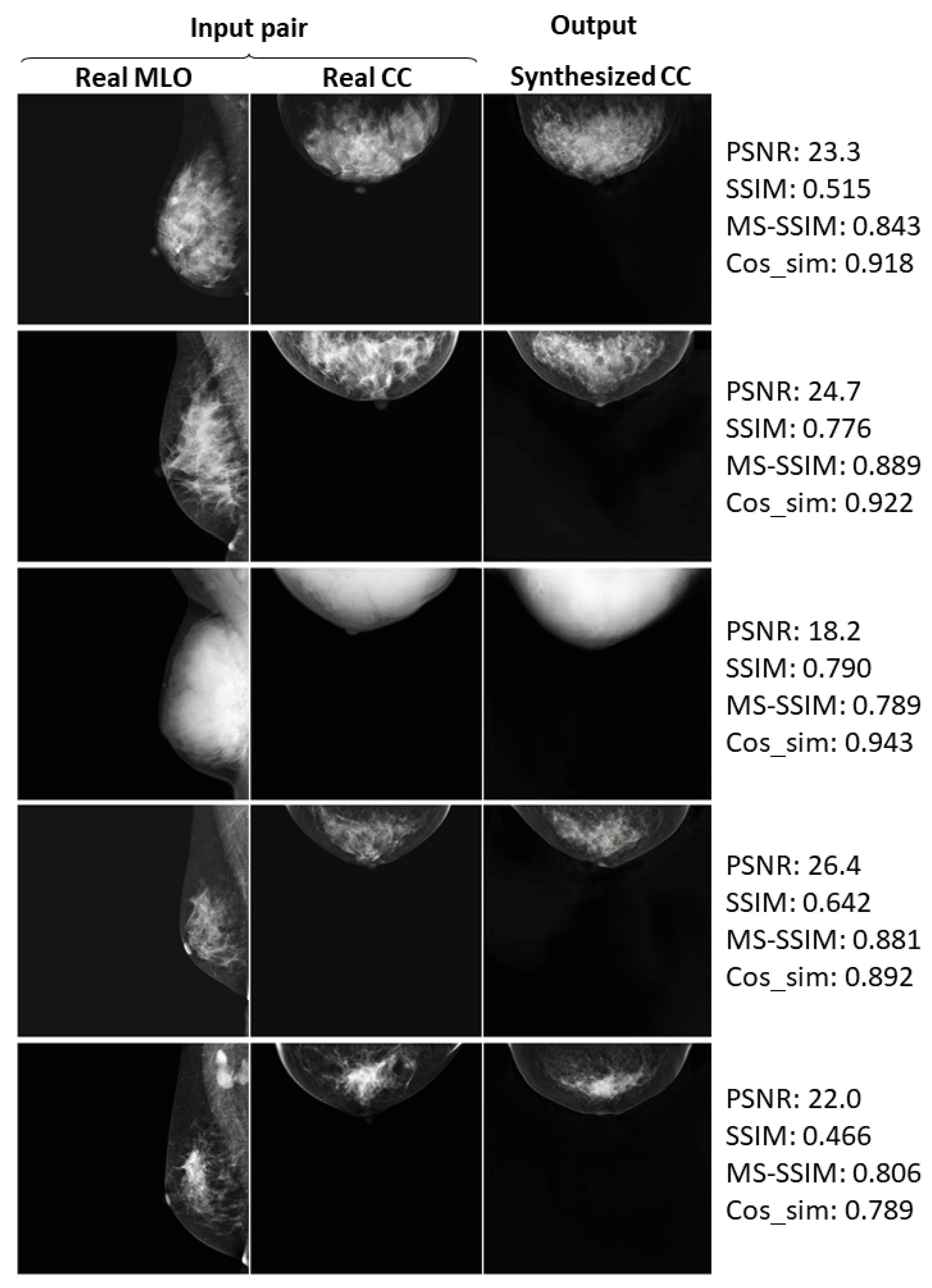
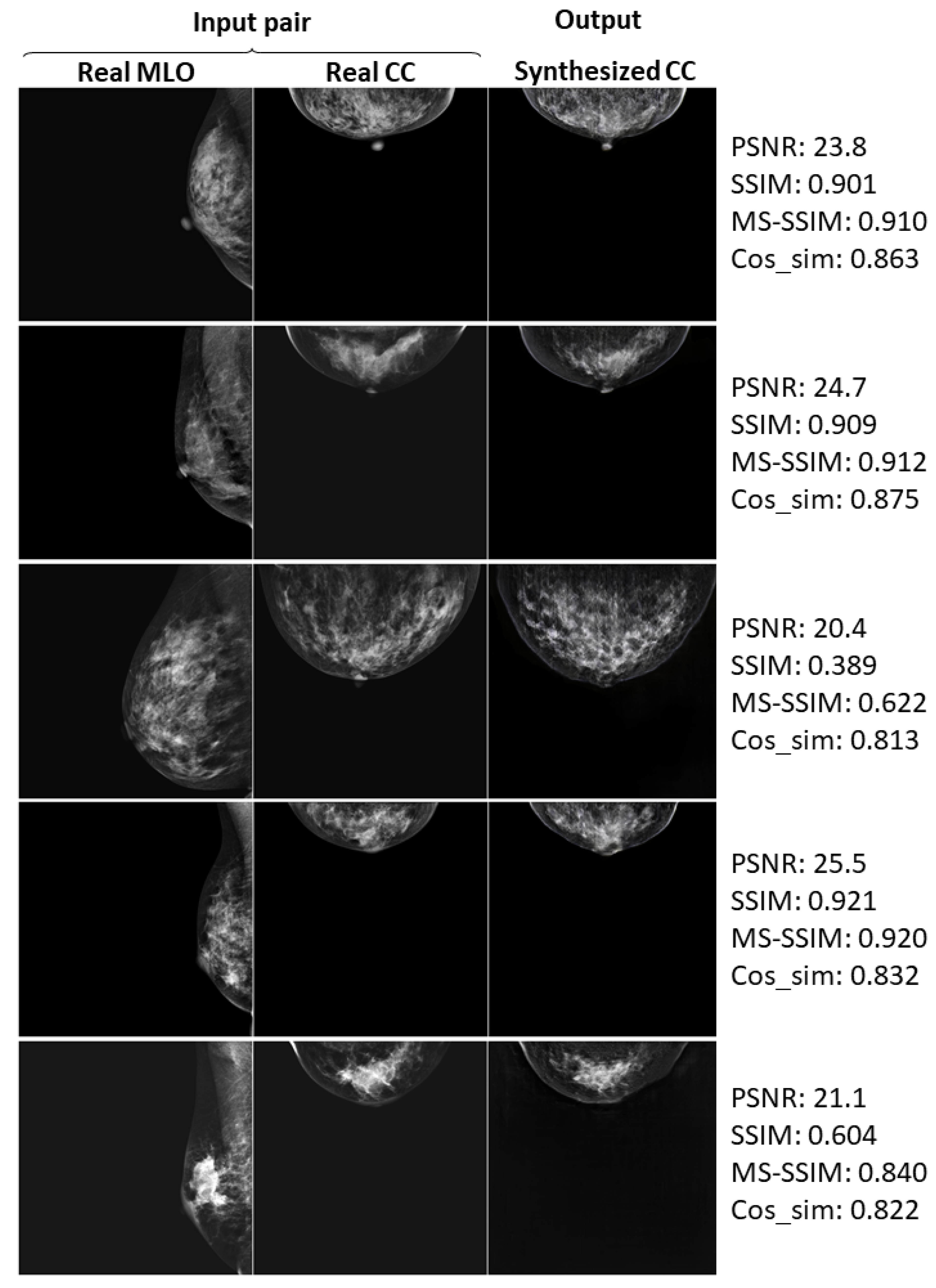
3.3. Successful and Failed Examples

Here, we again define successful cases, where the synthesized CC views look quite similar to the real ones. Figure 8, Figure 9 and Figure 10 show the successful examples at 128 × 128, 256 × 256, and 512 × 512 resolutions, respectively, using the method incorporating the PG technique and $L_{FM}$. The calculated similarity metrics are presented in the right columns. Further examples of relatively successful cases are shown in Figure A1–Figure A3 in the Appendix A. In contrast, examples, in which the real and synthesized CC views do not resemble each other, are defined as failed cases. Figure 11, Figure 12 and Figure 13 show the examples of failure at each resolution when using the method incorporating PG technique and $L_{FM}$. The authors, who are radiological technologists with more than 10 years of experience, judged whether the synthesized images belong to the successful or failed cases. A.Y. is also a mammography technologist certified by the Japan Central Organization on Quality Assurance of Breast Cancer Screening. The judgment was conducted by comparing the shape of the breast, the mammary-gland density and structure, the shape and size of the lesion, and other clinically important factors between the real and synthesized views. For instance, the synthesized view in which the mammary-gland density differs from the real view, or in which the tumor that should be there is missing, were included in the failed cases.

In Figure 8, Figure 9 and Figure 10, the synthesized CC views appear to be similar to the real views and preserve the identity well. Meanwhile, in other cases, such as the examples in Figure 11, Figure 12 and Figure 13, the identity is lost, and the synthesized views do not seem similar to images of the same subjects as the real views. Even in cases where the tumor is successfully represented, the tumor size and shape are not exactly the same as in the real image; for instance, see Figure 8a–c, Figure 9a–c, and Figure 10a,b,d. Moreover, image syntheses of calcifications were barely successful at all resolutions. In some cases of 512 × 512 resolution, the synthesized CC views presented remarkable artifacts, such as stripe lines, jagged textures, and defects in the breast area, as shown in Figure 13. Enlarged versions of the images in Figure 13e are provided in Figure 14. Despite the fact that the case has a large tumor covered with amorphous calcifications, the synthesized tumor looks different in size and shape from in the real image, and we cannot see calcifications covering the entire tumor. However, several small specks resembling calcifications appear, as indicated by the red arrows in Figure 14. Such specks are invisible in the synthesized views at 128 × 128 and 256 × 256 resolutions.

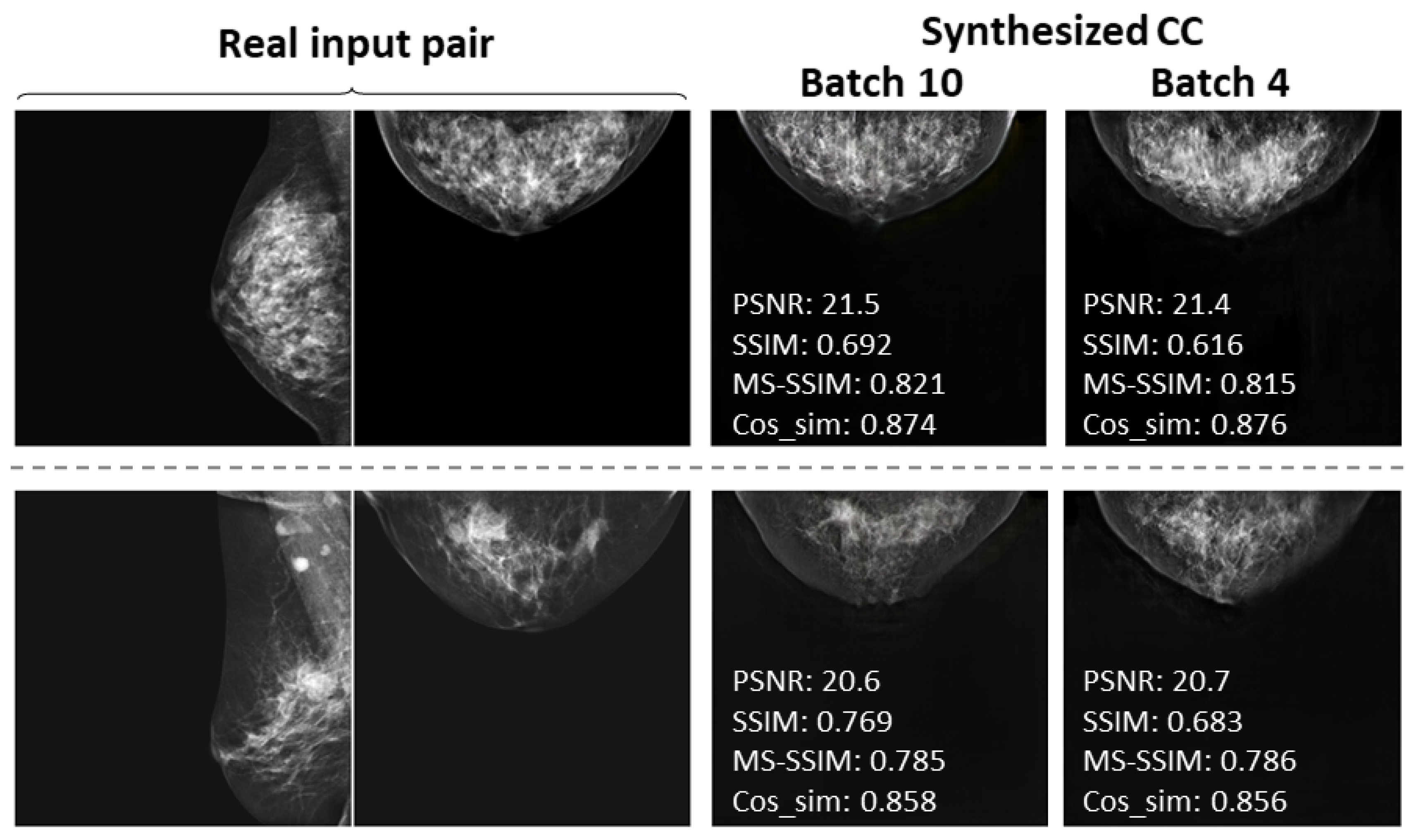
3.4. Comparison by Batch Size

We also found, as can be seen from Table 3, that the similarity metrics slightly decreased (PSNR, MS-SSIM, and Cos_sim: p < 0.05) and the training time considerably lengthened as the batch size changed from 10 to 4 for 256 × 256 image synthesis. Figure 15 shows the real input mammograms and the respective synthesized CC views using batch sizes of 10 and 4 for two case examples. We frequently observed that, when using a batch size of 4 (and not only in these two cases), there were more notable artifacts in the synthesized views, such as stripe lines and texture distortion in the mammary gland. In spite of the slight decreases in the similarity metrics, the use of a smaller batch size clearly degraded the image quality.

4. Discussion

In this study, we compared the performance of CR-GAN with that of our proposed methods for CC-view synthesis from MLO views. Our results revealed the disadvantages of the method using only CR-GAN, in terms of the synthesized image quality. We also found that training using only CR-GAN takes quite a long time as the synthesized image resolution increases. Subsequently, we incorporated the PG technique into CR-GAN, and confirmed that it brings significant benefits in reducing the training time, except for the case of 128×128 resolution. Additionally, the synthesized CC views came closer to the real views and the artifacts were less obvious with the adaptation of $L_{FM}$, as can be seen from Figure 6 and Figure 7, and the similarity metrics also increased the most in Table 3. Overall, our proposed method using both the PG technique and $L_{FM}$ offers the best performance, in terms of the image quality and training time, for high-resolution CC-view synthesis. Although the unidirectional training time may be substantially shorter, the image quality is inferior to that of bi-directional training.

Even with the approach utilizing the PG technique and $L_{FM}$, synthesis failed in some cases, as shown in Figure 11, Figure 12 and Figure 13. As such, complete representation—from which the name of CR-GAN is derived—has not been accomplished here. Notably, image synthesis was barely successful in cases of calcification. Nonetheless, the proposed method with the PG technique and $L_{FM}$ at 512 × 512 resolution provides a perspective on the calcification, as implied by the white specks in Figure 14. There is a limitation that the image quality was assessed by radiological technologists in this work. In fact, the diagnostic potential needs to be evaluated by radiologists or breast surgeons.

We consider the insufficient volume of training data and the restricted batch sizes as reasonable causes of synthesis failure. In Figure 15, it can also be seen that the artifacts were more noticeable and the image quality was degraded with lower batch size. According to [48], Tian et al. have successfully generated multi-view face images using labeled images of at least 200 subjects from Multi-PIE and 72,000 unlabeled images from CelebA [49] by CR-GAN with a batch size of 64. The number and variation of our used training data, consisting of images from approximately 3000 subjects, would surely have been too small to cover the whole latent space. Korkinof et al. [26] have synthesized realistic high-resolution mammograms at 1280 × 1240 resolution by PG-GAN using eight GPUs each with 16 GB memory. Although their used batch size was not specified, it is expected that they used batch sizes higher than 4, which was the available maximum batch size for the 512 × 512 image syntheses in our training environment using only one 16 GB GPU. In fact, the models without $L_{FM}$ using a batch size of 4 failed to synthesize 256 × 256 images, due to the divergence of discriminator and generator losses. This suggests that such a small batch size could cause instability in the training. Subsequently, synthesis of 512 × 512 images also resulted in failure, due to the same issue with the loss functions. We speculate that the small batch size makes the training unstable, potentially leading to the vanishing gradient problem. Taken together, we can expect improvements in the image quality if the training is performed with a larger image data set within a more powerful GPU environment. A powerful GPU would make it possible to apply larger batch sizes, and three or more vectors should be utilized in the $L_{FM}$ calculation for stronger constraints on middle-layer representations. It would also be feasible to synthesize images at resolutions higher than 512 × 512, which is essential for clinical mammograms. In addition, we did not conduct any validation to adjust the hyperparameters. By making such adjustments, the performance could be further improved, and this technology may eventually succeed in providing clinically acceptable CC views. As a result, the realization leads to the improved accuracy of breast cancer diagnosis by single-view mammography.

As can obviously be seen from Figure 6 and Figure 7, the sharpness was degraded in images synthesized using the method with the PG technique and without $L_{FM}$, compared with the method using only CR-GAN. Nevertheless, the sole adaptation of the PG technique increased some of the similarity metrics, as shown in in Table 3. While the image quality improvements by $L_{FM}$ were visually impressive, we wonder about the modest increases in the similarity metrics. We also noticed relatively low similarity metrics in some cases, despite the fact that the real and synthesized views looked quite similar, such as SSIM = 0.322 in Figure 8c and SSIM = 0.679 and MS-SSIM = 0.768 in Figure 10c. In contrast, some cases where the real and synthesized views looked dissimilar presented relatively high metrics, such as Cos_sim = 0.942 in Figure 11b; SSIM = 0.935, MS-SSIM = 0.910, and Cos_sim = 0.972 in Figure 12a; and SSIM = 0.916 and Cos_sim = 0.964 in Figure 13a. Hence, we must note that the metrics are not always congruent with how humans perceive similarity. Even though the SSIM is believed to be more consistent with human perception than PSNR [50], Pambrun et al. [51] have described some of the drawbacks of SSIM in medical imaging applications. They claimed that the SSIM is insensitive to high-intensity variations and tends to under-estimate distortion at high-frequency edges. Mudeng et al. [52] have also mentioned that SSIM has shortcomings, under-estimating spatial translation while over-estimating image blurring. High-frequency edges and high-intensity signals are particularly important features in mammograms. We can actually observe structural changes more complex than spatial translation in synthesized images using AI models, such as GANs. Accordingly, the SSIM can probably not be regarded as the optimal evaluation metric for our task. Although Mudeng et al. have predicted that improved SSIM metrics, including MS-SSIM, can overcome these issues, we noticed some drawbacks of MS-SSIM. As Cos_sim is often used for image classification of animals or fruits [46], we anticipated it focusing on rough and low-frequency features, rather than detailed structures. As a result, although Cos_sim often showed appropriately low values for missing large-tumor data or obvious mammary-density differences (refer to Figure 11d and Figure 12c,e), it was insensitive to artifacts such as stripe lines and defects, as indicated by the relatively high metrics in Figure 13a–c. In conclusion, we should investigate and discuss methods more faithful to human perception, in order to evaluate AI-generated medical images.

5. Conclusions

We adopted CR-GAN and incorporated two approaches (the PG technique and feature matching loss), in order to synthesize CC-view mammograms from MLO view data. We demonstrated that the PG technique can effectively reduce the training time, whereas use of the feature matching loss considerably improved the quality of the synthesized images. The proposed method succeeded in synthesizing CC views similar to the real images for some (but not all) cases. Our findings should serve as a technical guide for the clinical application of artificially synthesized two-view mammograms. We intend to improve the image quality and resolution by utilizing a larger image data set and optimized hyperparameters—including the batch size—in future work. Furthermore, we will conduct quantitative analyses using more faithful evaluation methods to human perception as well as subjective assessments by radiologists in terms of the clinical usefulness.

References

1. Terrasse, V. Latest global cancer data: Cancer burden rises to 19.3 million new cases and 10.0 million cancer deaths in 2020. In The International Agency for Research on Cancer Press Release 292; IARC: Lyon, France, 2020; pp. 1–3. [Google Scholar]
2. Sung, H.; Ferlay, J.; Siegel, R.L.; Laversanne, M.; Soerjomataram, I.; Jemal, A.; Bray, F. Global Cancer Statistics 2020: GLOBOCAN estimates of incidence and mortality worldwide for 36 cancers in 185 countries. CA Cancer J. Clin. 2021, 71, 209–249. [Google Scholar] [CrossRef] [PubMed]
3. Mayor, S. Survival of women treated for early breast cancer detected by screening is same as in general population, audit shows. BML 2008, 336, 1398–1399. [Google Scholar] [CrossRef] [PubMed] [Green Version]
4. Duffy, S.W.; Vulkan, D.; Cuckle, H.; Parmar, D.; Sheikh, S.; Smith, R.A.; Evans, A.; Blyuss, O.; Johns, L.; Ellis, I.O.; et al. Effect of mammographic screening from age 40 years on breast cancer mortality (UK Age trial): Final results of a randomised, controlled trial. Lancet Oncol. 2020, 21, 1165–1172. [Google Scholar] [CrossRef] [PubMed]
5. Hamashima, C.; Ohta, K.; Kasahara, Y.; Katayama, T.; Nakayama, T.; Honjo, S.; Ohnuki, K. A meta-analysis of mammographic screening with and without clinical breast examination. Cancer Sci. 2015, 106, 812–818. [Google Scholar] [CrossRef] [Green Version]
6. van den Ende, C.; Oordt-Speets, A.M.; Vroling, H.; van Agt, M.E. Benefits and harms of breast cancer screening with mammography in women aged 40–49 years: A systematic review. Int. J. Cancer 2017, 141, 1295–1306. [Google Scholar] [CrossRef] [Green Version]
7. Christiansen, S.R.; Autier, P.; Støvring, H. Change in effectiveness of mammography screening with decreasing breast cancer mortality: A population-based study. Eur. J. Public Health. 2022, 32, 630–635. [Google Scholar] [CrossRef]
8. Gossner, J. Digital mammography in young women: Is a single view sufficient? J. Clin. Diagn. Res. 2016, 10, TC10–TC12. [Google Scholar] [CrossRef]
9. Rubin, D. Guidance on Screening and Symptomatic Breast Imaging, 4th ed.; The Royal College of Radiologists: London, UK, 2019; pp. 1–27. [Google Scholar]
10. Sickles, E.A.; Weber, W.N.; Galvin, H.B.; Ominsky, S.H.; Sollitto, R.A. Baseline screening mammography: One vs two views per breast. Am. J. Roentgenol. 1986, 147, 1149–1155. [Google Scholar] [CrossRef] [Green Version]
11. Feig, S.A. Screening mammography: A successful public health initiative. Pan. Am. J. Public Health 2006, 20, 125–133. [Google Scholar] [CrossRef] [Green Version]
12. Ray, K.M.; Joe, B.N.; Freimanis, R.I.; Sickles, E.A.; Hendrick, R.E. Screening mammographyin women 40-49 years old: Current evidence. Am. J. Roentgenol. 2018, 210, 264–270. [Google Scholar] [CrossRef]
13. Kasumi, F. Problems in breast cancer screening. Jpn. Med. Assoc. J. 2005, 48, 301–309. [Google Scholar]
14. Tsuchida, J.; Nagahashi, M.; Rashid, O.M.; Takabe, K.; Wakai, T. At what age should screening mammography be recommended for Asian women? Cancer Med. 2015, 4, 1136–1144. [Google Scholar] [CrossRef]
15. Helme, S.; Perry, N.; Mokbel, K. Screening mammography in women aged 40–49: Is it time to change? Int. Semin. Surg. Oncol. 2006, 3, 1–4. [Google Scholar] [CrossRef] [PubMed] [Green Version]
16. Giess, C.S.; Frost, E.P.; Birdwell, R.L. Interpreting one-view mammographic findings: Minimizing callbacks while maximizing cancer detection. RadioGraphics. 2014, 34, 928–940. [Google Scholar] [CrossRef] [PubMed]
17. Litjens, G.; Kooi, T.; Bejnordi, B.E.; Setio, A.A.A.; Ciompi, F.; Ghafoorian, M.; van der Laak, J.A.W.M.; van Ginneken, B.; Sánchez, C.I. A survey on deep learning in medical image analysis. Med. Image Anal. 2017, 42, 60–88. [Google Scholar]
18. Bakator, M.; Radosav, D. Deep learning and medical diagnosis: A review of literature. Multimodal Technol. Interact. 2018, 2, 47. [Google Scholar] [CrossRef] [Green Version]
19. Sahiner, B.; Pezeshk, A.; Hadjiiski, L.M.; Wang, X.; Drukker, K.; Cha, K.H.; Summers, R.M.; Giger, M.L. Deep learning in medical imaging and radiation therapy. Med. Phys. 2019, 46, e1–e36. [Google Scholar] [CrossRef] [Green Version]
20. Goodfellow, I.; Pouget-Abadie, J.; Mirza, M.; Xu, B.; Warde-Farley, D.; Ozair, S.; Courville, A.; Bengio, Y. Generative adversarial nets. In Advances in Neural Information Processing Systems (NIPS 2014); NeurIPS: San Diego, CA, USA, 2014; pp. 2672–2680. [Google Scholar]
21. Kingma, D.P.; Welling, M. Auto-encoding variational bayes. arXiv 2013, arXiv:1312.6114. [Google Scholar]
22. Arjovsky, M.; Chintala, S.; Bottou, L. Wasserstein generative adversarial networks. In Proceedings of the 34th International Conference on Machine Learning, Sydney, Australia, 6–11 August 2017; pp. 214–223. [Google Scholar]
23. Karras, T.; Aila, T.; Laine, S.; Lehtinen, J. Progressive growing of gans for improved quality, stability, and variation. In Proceedings of the Sixth International Conference on Learning Representations (ICLR), Vancouver, BC, Canada, 30 April–3 May 2018; pp. 1–26. [Google Scholar]
24. Karras, T.; Laine, S.; Aittala, M.; Hellsten, J.; Lehtinen, J.; Aila, T. Analyzing and improving the image quality of StyleGAN. In Proceedings of the 2020 IEEE/CVF Conference on Computer Vision and Pattern Recognition (CVPR), Seattle, WA, USA, 13–19 June 2020; pp. 8107–8116. [Google Scholar]
25. Lee, J.; Nishikawa, R.M. Identifying women with mammographically- occult breast cancer leveraging GAN- simulated mammograms. IEEE Trans. Med. Imaging 2022, 41, 225–236. [Google Scholar] [CrossRef]
26. Korkinof, D.; Rijken, T.; O’Neill, M.; Yearsley, J.; Harvey, H.; Glocker, B. High-resolution mammogram synthesis using progressive generative adversarial networks. arXiv 2018, arXiv:1807.03401. [Google Scholar]
27. Oyelade, O.N.; Ezugwu, A.E.; Almutairi, M.S.; Saha, A.K.; Abualigah, L.; Chiroma, H. A generative adversarial network for synthetization of regions of interest based on digital mammograms. Sci. Rep. 2022, 12, 6166. [Google Scholar] [CrossRef]
28. Tran, L.; Yin, X.; Liu, X. Disentangled representation learning GAN for pose-invariant face recognition. In Proceedings of the 2017 IEEE Conference on Computer Vision and Pattern Recognition (CVPR), Honolulu, HI, USA, 21–26 July 2017; pp. 1283–1292. [Google Scholar]
29. Zhao, B.; Wu, X.; Cheng, Z.; Liu, H.; Jie, Z.; Feng, J. Multi-view image generation from a single-view. arXiv 2018, arXiv:1704.04886. [Google Scholar]
30. Heo, Y.; Kim, B.; Roy, P.P. Frontal face generation algorithm from multi-view images based on generative adversarial network. J. Multimed. Inf. Syst. 2021, 8, 85–92, ISSN: 2383–7632. [Google Scholar] [CrossRef]
31. Zou, H.; Ak, K.E.; Kassim, A.A. Edge-Gan: Edge conditioned multi-view face image generation. In Proceedings of the 2020 IEEE International Conference on Image Processing (ICIP), Abu Dhabi, United Arab Emirates, 25–28 October 2020; pp. 2401–2405. [Google Scholar]
32. Tian, Y.; Peng, X.; Zhao, L.; Zhang, S.; Metaxas, D.N. CR-GAN: Learning complete representations for multi-view generation. arXiv 2018, arXiv:1806.11191. [Google Scholar]
33. Jahanian, A.; Puig, X.; Tian, Y.; Isola, P. Generative models as a data source for multiview representation learning. arXiv 2021, arXiv:2106.05258. [Google Scholar]
34. bluer555/CR-GAN. Available online: https://github.com/bluer555/CR-GAN (accessed on 31 October 2022).
35. Gulrajani, I.; Ahmed, F.; Arjovsky, M.; Dumoulin, V.; Courville, A. Improved training of Wasserstein GANs. In NeurIPS Proceedings; NeurIPS: San Diego, CA, USA, 2017; pp. 5769–5779. [Google Scholar]
36. Wang, T.; Liu, M.; Zhu, J.; Tao, A.; Kautz, J.; Catanzaro, B. High-resolution image synthesis and semantic manipulation with conditional gans. In Proceedings of the 2018 IEEE/CVF Conference on Computer Vision and Pattern Recognition, Salt Lake City, UT, USA, 18–23 June 2018; pp. 8798–8807. [Google Scholar]
37. Johnson, J.; Alahi, A.; Fei-Fei, L. Perceptual losses for real-time style transfer and super-resolution. In Lecture Notes in Computer Science; Springer: Cham, Switzerland, 2016; pp. 694–711. [Google Scholar]
38. Donahue, J.; Krähenbühl, P.; Darrell, T. Adversarial feature learning. arXiv 2016, arXiv:1605.09782. [Google Scholar]
39. Lee, R.S.; Gimenez, F.; Hoogi, A.; Miyake, K.K.; Gorovoy, M.; Rubin, D.L. A curated mammography data set for use in computer-aided detection and diagnosis research. Sci. Data. 2017, 4, 170177. [Google Scholar] [CrossRef] [Green Version]
40. Inês, C.M.; Igor, A.; Hoogi, A.; Inês, D.; António, C.; Maria, J.C.; Jaime, S.C. INbreast: Toward a full-field digital mammographic database. Acad. Radiol. 2012, 19, 236–248. [Google Scholar]
41. The Chinese Mammography Database (CMMD). Available online: https://wiki.cancerimagingarchive.net/pages/viewpage.action?pageId=70230508 (accessed on 31 October 2022).
42. Heusel, M.; Ramsauer, H.; Unterthiner, T.; Nessler, B.; Hochreiter, S. GANs trained by a two time-scale update rule converge to a local nash equilibrium. In Advances in Neural Information Processing Systems (NIPS 2017); NeurIPS: San Diego, CA, USA, 2017; pp. 6626–6637. [Google Scholar]
43. Borji, A. Pros and cons of GAN evaluation measures. arXiv 2018, arXiv:1802.03446. [Google Scholar] [CrossRef]
44. Wang, Z.; Bovik, A.C.; Sheikh, H.R.; Simoncelli, E.P. Image quality assessment: From error measurement to structural similarity. IEEE Trans. Image Process. 2004, 13, 600–612. [Google Scholar] [CrossRef] [Green Version]
45. Wang, Z.; Simoncelli, E.P.; Bovik, A.C. Multiscale structural similarity for image quality assessment. In Proceedings of the 37th IEEE Asilomar Conference on Signals, Systems & Computers, Pacific Grove, CA, USA, 9–12 November 2003; Volume 2, pp. 1398–1402. [Google Scholar]
46. Jaiswal, A.; Babu, A.R.; Zadeh, M.Z.; Banerjee, D. A survey on contrastive self-supervised learning. arXiv 2021, arXiv:2011.00362. [Google Scholar] [CrossRef]
47. Chen, T.; Kornblith, S.; Norouzi, M.; Hinton, G. A simple framework for contrastive learning of visual representations. arXiv 2020, arXiv:2002.05709. [Google Scholar]
48. Gross, R.; Matthews, I.; Cohn, J.; Kanade, T.; Baker, S. Multi-PIE. Image Vis. Comput. 2010, 25, 807–813. [Google Scholar] [CrossRef] [PubMed]
49. Liu, Z.; Luo, P.; Wang, X.; Tang, X. Deep learning face attributes in the wild. In Proceedings of the 2015 IEEE International Conference on Computer Vision (ICCV), Santiago, Chile, 7–13 December 2015; pp. 3730–3738. [Google Scholar]
50. Umme, S.; Morium, A.; Mohammad, S.U. Image quality assessment through FSIM, SSIM, MSE and PSNR—A comparative study. J. Comput. Commun. 2019, 7, 8–18. [Google Scholar]
51. Pambrun, J.-F.; Noumeir, R. Limitations of the SSIM quality metric in the context of diagnostic imaging. In Proceedings of the 2015 IEEE International Conference on Image Processing (ICIP), Quebec City, QC, Canada, 27–30 September 2015; pp. 2960–2963. [Google Scholar]
52. Mudeng, V.; Kim, M.; Choe, S. Prospects of structual similarity index for medical image analysis. Appl. Sci. 2022, 12, 3754. [Google Scholar] [CrossRef]
Figure 1. Our training networks based on the CR-GAN framework. In the reconstruction path, the inputs and outputs of each network vary, depending on whether there is a forward learning or inverse mapping case.
Applsci 12 12206 g001
Figure 2. Gradually increasing image resolution in the generator, discriminator, and encoder as training advances through the progressive growing technique.
Applsci 12 12206 g002
Figure 3. Resolution transition in the progressive growing technique. This is an example of the transition from 64 × 64 to 128 × 128 resolution. When a new layer generating a 128 × 128 feature vector is inserted into the generator, a 64 × 64 feature vector from the last layer is 2× up-sampled using the bilinear method. The up-sampled vector weighted by (1- α ) and the newly inserted vector weighted by α are summed. In the discriminator and encoder, the newly inserted 128 × 128 image is translated to a feature vector with 64 channels and then down-scaled, using the nearest neighbor method, to 64 × 64 resolution. The weighted downscaled vector and vector from the next layer are also summed.
Applsci 12 12206 g003
Figure 4. Calculation of feature matching loss ( L F M ) using feature vectors from middle layers of the discriminator. When an image with a resolution ranging from 32 × 32 to 128 × 128 is input into the discriminator, three feature vectors ( D 1 , D 2 , D 3 ) are used to calculate L F M . The shape of D 1 depends on the input image size. When a 256 × 256 or 512 × 512 image is input into the discriminator, L F M is calculated from two vectors with shape 128 × 128 × 64 and 8 × 8 × 512, respectively.
Applsci 12 12206 g004
Figure 5. Pre-processing flow for training. Mammograms from each database were converted into 8-bit PNG images with 512 × 512 resolution. Data augmentation was applied to quadruple the number of training data pairs from CBIS-DDSM and INBreast. The orientations of all CC images were unified to be similar to frontal face photographs. Left MLO images were horizontally flipped to have the same orientation as right MLO images.
Applsci 12 12206 g005
Figure 6. Comparison of CC views at 128 × 128 resolution synthesized by training methods. Examples chosen of a successful case using bi-directional training with PG technique and feature matching loss. The yellow arrows indicate artifacts outside the breast.
Applsci 12 12206 g006
Figure 7. Comparison of synthesized CC views at 256 × 256 resolution by training methods. Examples chosen of a successful case using bi-directional training with PG technique and feature matching loss. The yellow arrows indicate artifacts outside the breast.
Applsci 12 12206 g007
Figure 8. Five successful examples (ae) of the real input paired and synthesized CC-view mammograms at 128 × 128 resolution by bi-directional training of CR-GAN incorporating PG technique and feature matching loss.
Applsci 12 12206 g008
Figure 9. Five successful examples (ae) of the real input paired and synthesized CC-view mammograms at 256 × 256 resolution by bi-directional training of CR-GAN incorporating PG technique and feature matching loss.
Applsci 12 12206 g009
Figure 10. Five successful examples (ae) of the real input paired and synthesized CC-view mammograms at 512 × 512 resolution by bi-directional training of CR-GAN incorporating PG technique and feature matching loss.
Applsci 12 12206 g010
Figure 11. Five failed examples (ae) of the real input paired and synthesized CC-view mammograms at 128 × 128 resolution by bi-directional training of CR-GAN incorporating PG technique and feature matching loss.
Applsci 12 12206 g011
Figure 12. Five failed examples (ae) of the real input paired and synthesized CC-view mammograms at 256 × 256 resolution by bi-directional training of CR-GAN incorporating PG technique and feature matching loss.
Applsci 12 12206 g012
Figure 13. Five failed examples (ae) of the real input paired and synthesized CC-view mammograms at 512 × 512 resolution by bi-directional training of CR-GAN incorporating PG technique and feature matching loss.
Applsci 12 12206 g013
Figure 14. Enlarged views of Figure 13e. The red arrows indicate specks corresponding to calcifications. The yellow arrows indicate stripe artifacts.
Applsci 12 12206 g014
Figure 15. Comparison of examples synthesized CC views at 256 × 256 resolution by batch size.
Applsci 12 12206 g015