1. Introduction
The energy transition is one of the great challenges of our society at the beginning of this millennium. To this, it must be added that the latest international socio-political events have exacerbated the energy crisis, evidencing the need for an acceleration in this transition. The electrical grid, as it has been known so far, is changing. It is evolving from a centralized to a more decentralized layout [
1], where priority is given to the consumption of energy coming from renewable energy sources. It has been shown that a restructuring of the electrical grid into local micro-grids makes it possible for greater integration of the amount of energy from renewable [
2,
3]. In particular, given its great potential for installation on building roofs, photovoltaic (PV) energy is becoming the most widely extended one [
4]. In this context, due to the increasing price of electricity and government subsidies for financing PV installations, these facilities are paying for themselves more quickly than ever, especially in the frame of self-consumption. Self-consumption or collective self-consumption (CSC), as its name suggests, is related to the consumption of local electricity production. In the Spanish state, according to data recorded by the Spanish Photovoltaic Union (UNEF), 1203 MW of new PV capacity was installed in 2021 in self-consumption facilities. This figure represents an increase in 101.8% compared to 2020 when 596 MW were commissioned [
5].
This research study has been developed in the framework of the EKATE project, an InterregPoctefa type program. EKATE is a project for PV electricity management and CSC in the France-Spain cross-border area, using Blockchain and Internet of Things (IoT) technologies [
6]. One of the pilot projects being developed within the framework of EKATE takes place in the Izarbel technology park in Bidart (France), involving the buildings of ESTIA Technology Institute. This Izarbel pilot project aims to implement innovative energy management in buildings in a CSC operation. In order to maximize the self-consumption rate and, as far as possible, energy efficiency, two types of energy management systems (EMS) are being designed and developed to be applied in the ESTIA2 building. To achieve the aforementioned objectives, these EMSs act on flexible loads (FL). What is known as demand side management (DSM) or demand response (DR)? For that, two types of FL have been considered, the Heating, Ventilation, and Air Conditioning (HVAC) system and the energy consumption behavior of the building users. Regarding the two EMSs designed:
(1) The first one is based on simple logic rules that act on the ON/OFF status of the internal HVAC units and/or on the temperature setpoints of the system and also influences the ESTIA2 user’s behavior in real-time according to the instantaneous surplus of PV energy.
(2) The second one is an intelligent EMS based on predictive models of ESTIA2 consumption and ESTIA1 PV production, a thermal model of ESTIA2 and HVAC, and an optimization algorithm.
This work complements a previously developed one, as shown in [
7], where three prediction models based on artificial intelligence (AI) are developed to predict the consumption of the ESTIA2 building.
The prediction of energy generation from renewable sources is not a new challenge. Different strategies can be found in the literature. Some works choose to predict the meteorological variables that influence energy production, such as solar radiation, temperature, or the clear sky index [
8,
9]. Afterward, in some cases, they use equations to calculate the corresponding energy generation. Whilst other works propose to directly predict the PV generation [
10,
11].
Another possible criterion for classifying prediction techniques is according to the type of model used. They are generally divided into three types: physical or analytical methods, recurrent methods, and AI-based methods. A physical method describes the atmospheric dynamics and physical states by a set of mathematical equations. This kind of model was the former one used for the forecasting of meteorological variables and PV generation. They are more trustworthy in the long-term forecast when weather conditions are more stable, as they do not behave well in the face of sudden changes. A drawback of physical techniques is that a thorough knowledge of physics is essential. Among the most know methods are numerical weather prediction (NWP) [
12] and sky imagery [
13]. As for recurrent methods, they have been the most widely used for time series forecasting for several years. Nevertheless, recurrent models can show problems in dealing with the non-linearity and seasonality properties [
14]. Finally, AI methods, contrary to recurrent methods, are indeed able to handle non-linear problems; thanks to this ability and to learning algorithms, AI methods can provide precise predictions and react to sudden meteorological changes. The researchers of [
15] provide an extensive review of AI-based solar energy prediction. They conclude that the most frequently applied techniques are artificial neural networks (ANN) in first place, followed by support vector machine (SVM) techniques.
Finally, another term by which PV generation predictors are also divided is by time horizon. The time horizon is the amount of time to forecast. In the literature, they are usually divided into three categories [
16]; (1) Short-term forecasting is considered to be between a few minutes and a week. Its function is to schedule energy transfer, demand response, and economic dispatch of load [
17]. (2) Medium-term forecasting is typically between 1 month and one year and is used to plan the next energy plans. (3) Long-term forecasting is usually considered when it is longer than one year, usually to plan the power plant to meet future needs and cost efficiency [
18].
This article presents four short-term PV generation, prediction models. One of them is an analytical model, and the other three are AI-based models. The overall objective of this paper is to design and compare different prediction models, with the goal of obtaining an accurate model that can be integrated into an EMS. A detailed explanation of how the models have been developed is given. The results are analyzed in different ways. On the one hand, the general behavior of the four models during one month is studied and compared to real data, and on the other hand, the analysis of the behavior of the models for different types of days, differentiating between sunny and cloudy days, is presented.
The remaining sections of the current article are organized as follows:
Section 2 describes the case study for which the four PV energy generation forecasters have been implemented. Afterward,
Section 3 explains the theory behind the techniques used to build the models. The development of the four models is described in
Section 4.
Section 5 presents the results obtained. Finally,
Section 6 discusses the obtained conclusions.
2. Case Study
This next section describes the real case study in which the models will be implemented. The first sub-section describes the characteristics of the site and the buildings that take part in the CSC. Furthermore, the second sub-section presents the features and the source of the data used in the development of the four models.
2.1. Izarbel Pilot Project Description
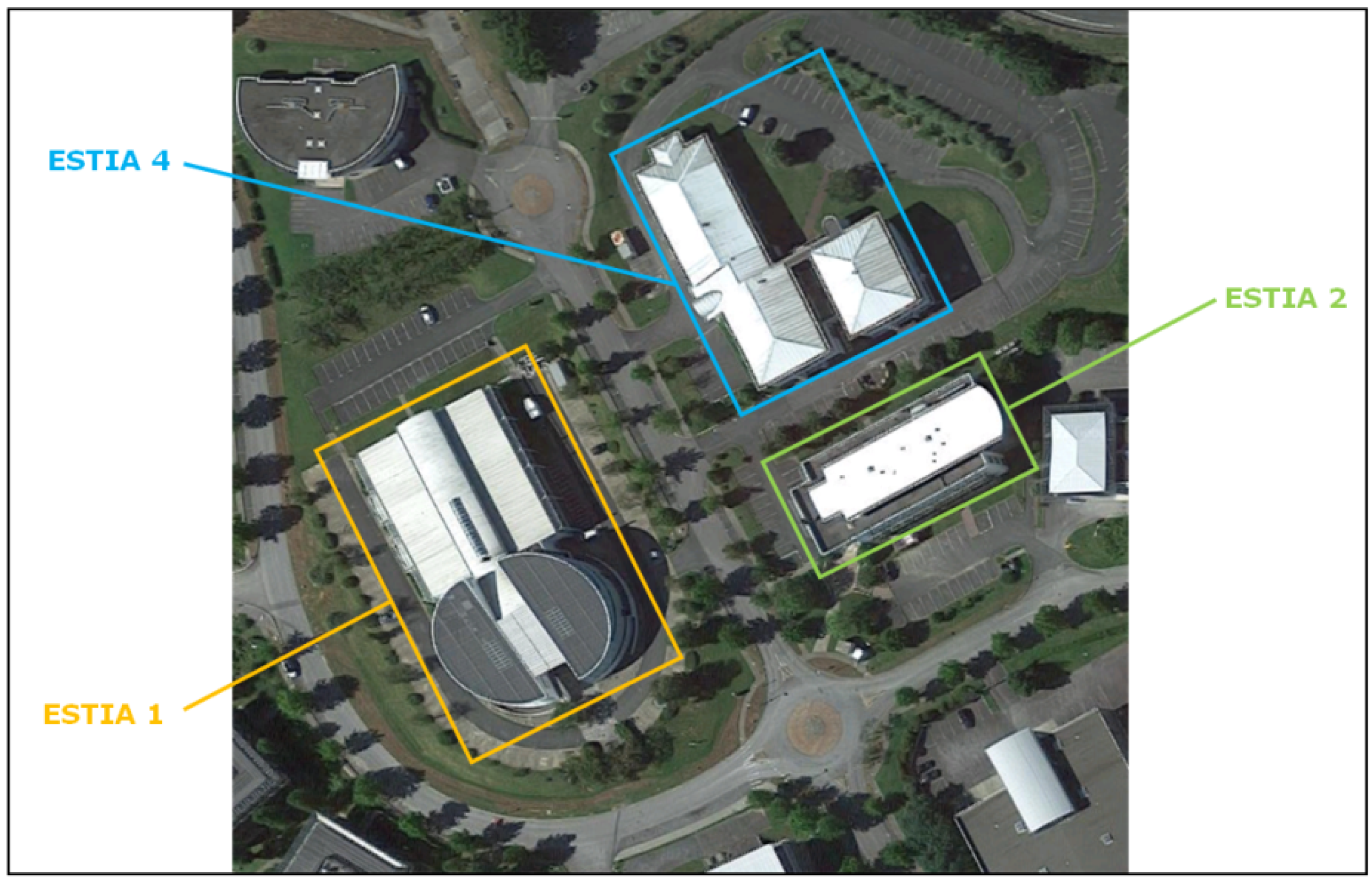
As previously mentioned, this pilot project has been carried out at the Izarbel technology park in Bidart, France. The PV energy CSC demonstrator is composed of three buildings, which are managed by the ESTIA Institute of Technology.
Figure 1 shows the buildings participating in the CSC.
Within the framework of the EKATE project, a total of 286 kWp of PV panels will be installed in these three buildings. Initially, the circular part of the ESTIA1 building will be equipped with an installation of 117.17 kWp. The rest of the PV installation will be carried out at a later stage in the ESTIA2 and ESTIA4 buildings. It should be noted that the 117.17 kWp installation has not yet been completed. However, data from a 2004 PV installation of 5.6 kWp capacity have been used to develop the PV generation, prediction models. The 5.6 kWp installation is not part of the CSC and is located on the circular part of the roof of the ESTIA1 building, with a southeast orientation and a slope of 20%.
2.2. Used Data Set
PV production data are collected via a Linky smart meter and are stored on a server in the cloud. These data started to be registered in April 2021 and are recorded every 30 min, i.e., 48 data sets per day.
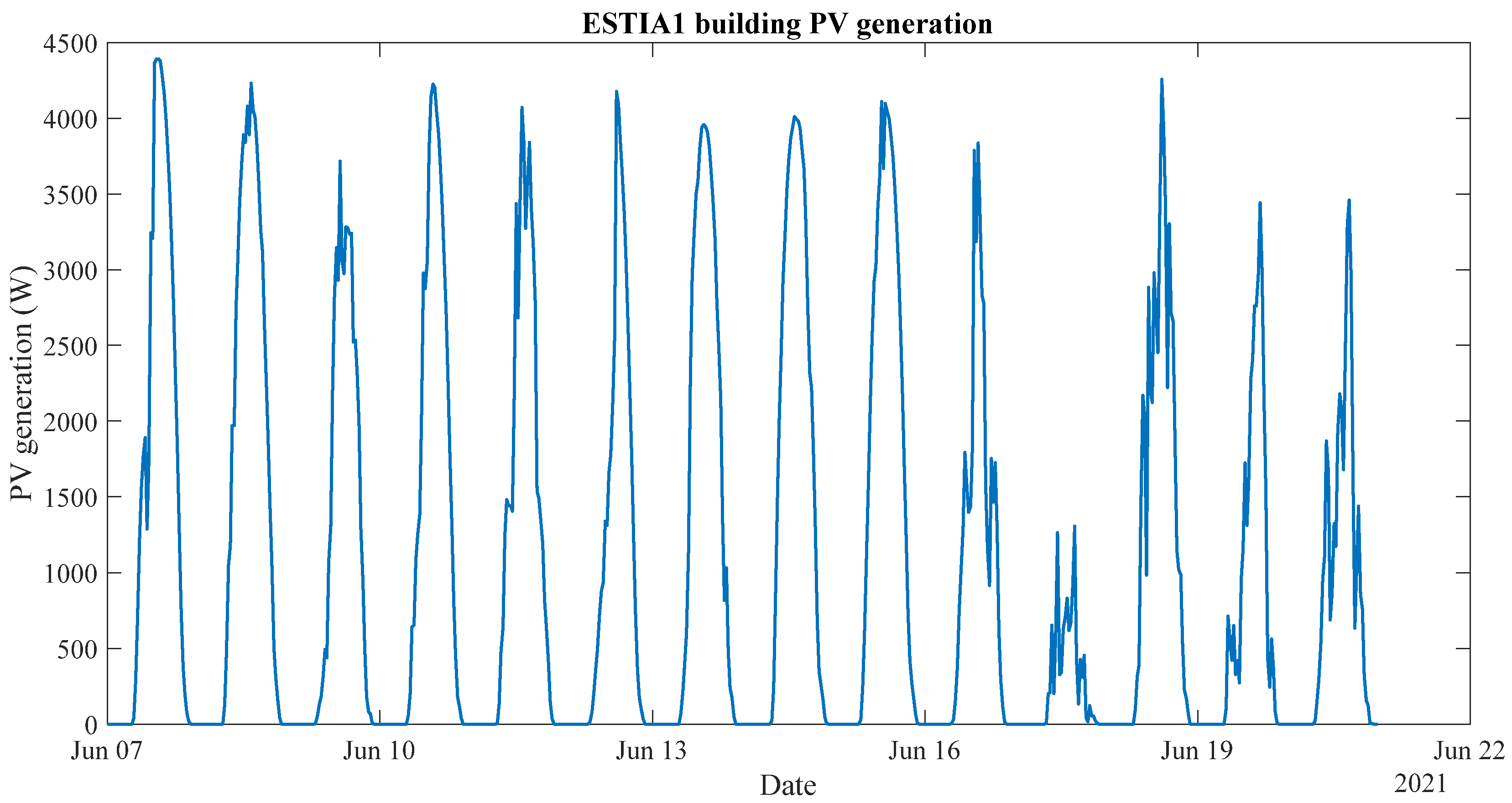
Figure 2 shows the PV production for 15 days in June. The production pattern is as expected, a null generation at night and a bell-shaped production during the day, where the maximum generation occurs at noon.
Figure 2 shows two types of days; sunny days, where the production is more constant, as seen in the characteristic bell shape, and more cloudy days, where the production is more irregular and saw-toothed. July PV production data have been forecasted for all four models.
Some meteorological data related to PV production have also been used in the development of the four models: irradiation, temperature, wind speed, and wind direction. These data have been obtained from the Météo France weather station. The closest station to the PV installation is the one located at Biarritz airport, approximately 3 km from the ESTIA1 building. The downloaded historical measured data have been recorded every hour, i.e., 24 data sets per day.
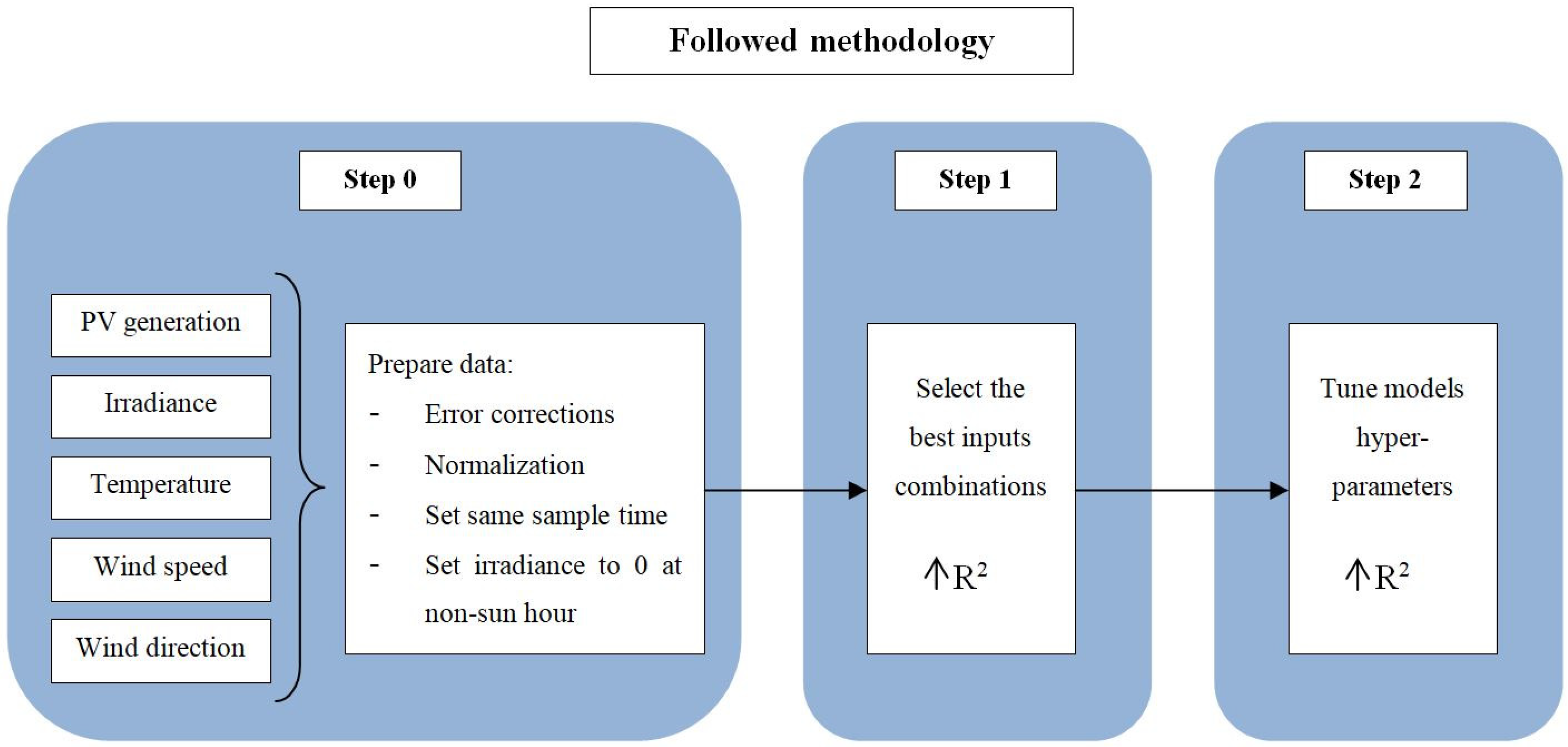
That one of the most important matters when developing data-based models is data quality, and thus, data pre-processing, all the data have been analyzed, and various filters have been applied to the collected database. Firstly, all data—PV production and meteorological data—have been analyzed to detect and repair possible outliers by interpolation. In case of duplicate data, these have been removed, and missing point data have been repaired by interpolation. Concerning solar irradiance, as mentioned above, the station that collects these data is located at an airport, so powerful light sources that are used near the station can alter the measured values of solar irradiance, especially at night when the lights are in operation. In order to remedy this potential problem, the sunrise and sunset times have been checked to determine a night time slot in which all solar irradiance values are replaced by zero. This range for the month of July has been set between 22:00 PM and 06:30 AM. Moreover, it is worth mentioning that once the prediction is made, in the post-processing of the data, the same filter is applied.
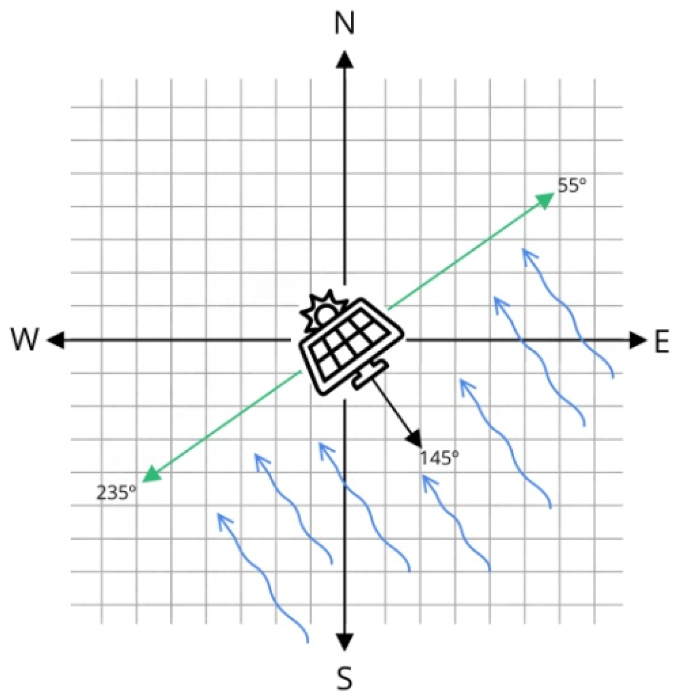
Furthermore, since wind speed reduces the temperature of the PV cell, it has been proposed to use two different vectors representing the wind. On the one hand, the wind coming from all directions will be used. On the other hand, it has been proposed to consider only the wind that directly hits the PV panels.
Figure 3 shows how the panels are oriented to the southeast, at 145° with respect to the north. As mentioned above, the roof on which the panels are located is slanted, so the wind coming from the back of the panels does not affect it. Therefore, by means of a weighting system, the wind coming from between 55° and 235° has been multiplied by 1, and the wind coming from the rest of the angles has been multiplied by 0. The direction-weighted wind speed has been used in the AI models.
Finally, all data have been set with the same sampling time. It has been decided to make the predictions every 30 min. Therefore, the hourly recorded meteorological data have been interpolated to obtain data every 30 min. Furthermore, all data have been normalized between the range 0 and 1. Normalization helps in the training period of the models. Indeed, if the range of values to be used was very different, a small learning rate value would be used, increasing the training time. On the other hand, if the range of all values is the same, the model can use an appropriate learning rate for all data and therefore reduce the training time.
3. PV Generation Forecaster Models
This section presents the theoretical fundaments of the models that have been developed to predict PV generation. The first described model is an analytical model developed in the OpenModelica software. The other three models are AI techniques, namely a feedforward neural network (FFNN), a nonlinear autoregressive with exogenous inputs (NARX) neural network, and a support vector regression (SVR).
3.1. Analytical Model
Analytical models are mathematical models that can be applied to address various working conditions, thanks to some assumptions that are made about the way a process evolves. The strength of the analytical model is that it provides a generic way of obtaining results for various conditions using a mathematical formulation. One of the disadvantages of analytical models is that they are often very difficult to obtain mathematically. Therefore, the accuracy of the model will depend on the validity of the assumptions made during the mathematical formulation. Analytical models can be further classified as static or dynamic. A static model represents properties of a system that are independent of time or true for any point in time. A dynamic model is an analytical model that represents the time-varying state of the system, such as its acceleration, velocity, and position as a function of time [
19].
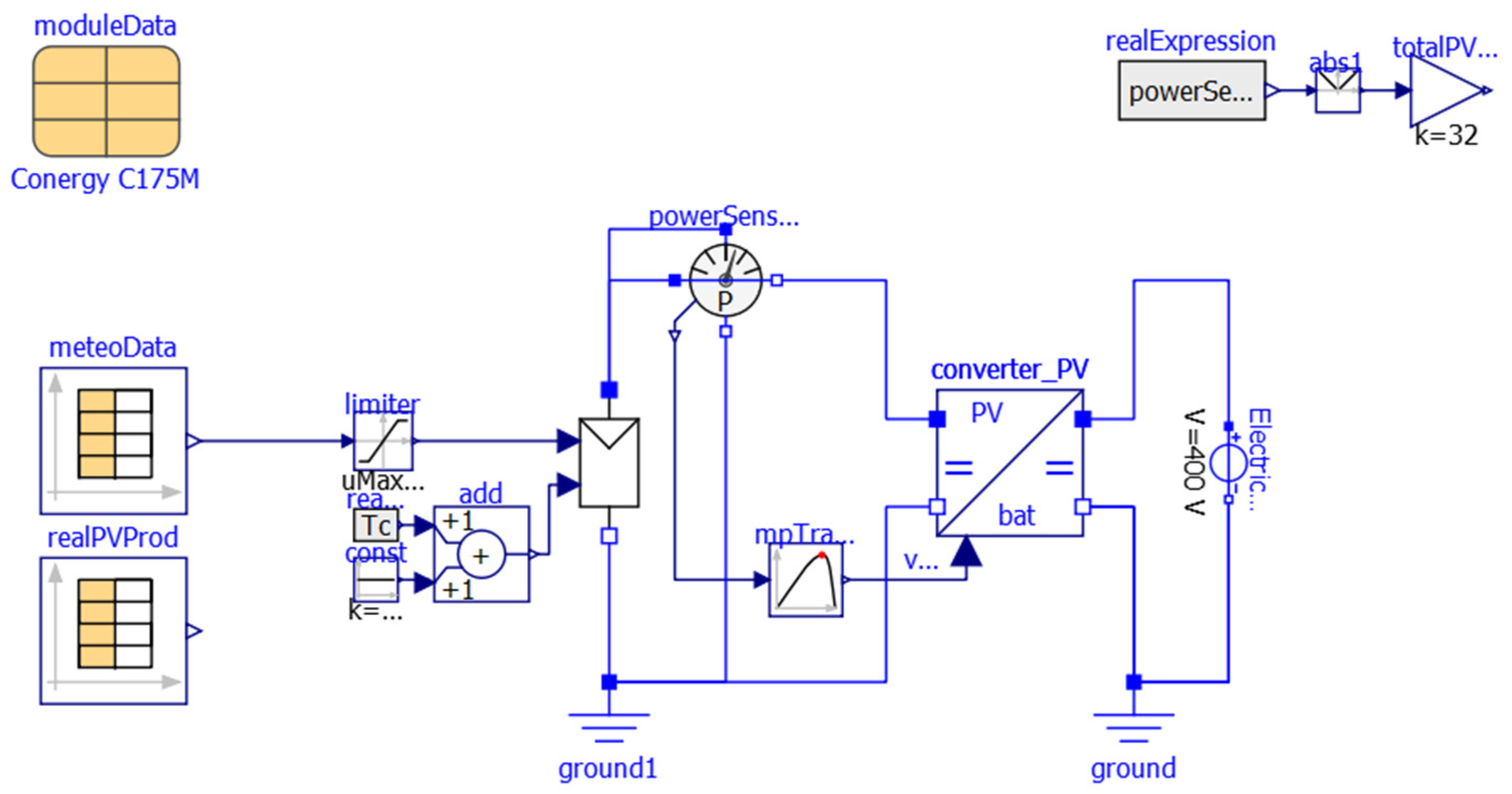
Modelica language has been chosen to implement the PV generation model. Modelica aims at acausal (non-causal) modeling of systems involving various physical domains by expressing them in the form of ordinary differential and algebraic equations [
20]. The model has been developed with the open-source software OpenModelica.
3.2. Artificial Intelligence Models
3.2.1. Feed Forward Neural Network
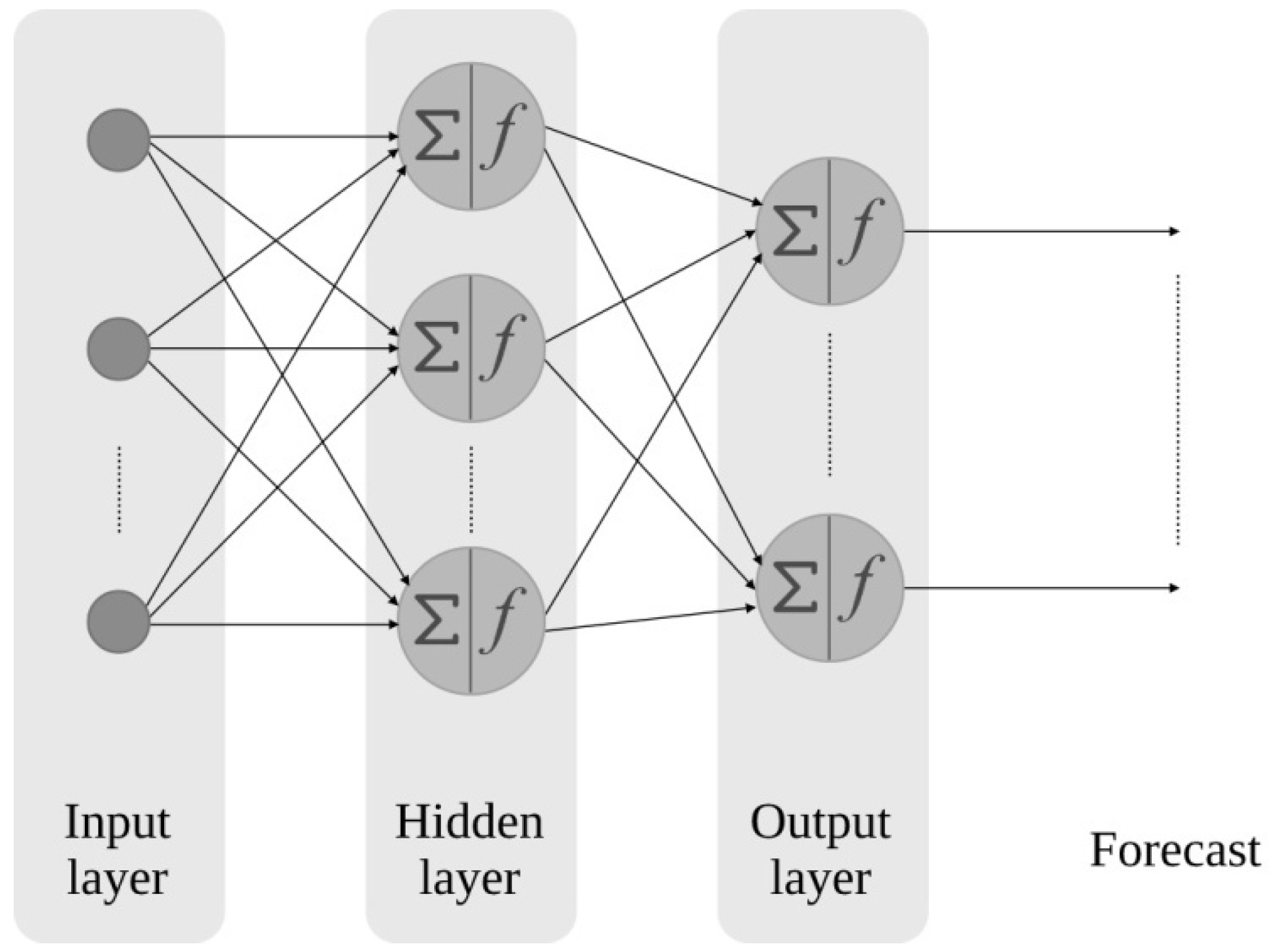
An FFNN is the simplest model of an ANN. Therefore, it also represents the definition of the ANN, and its main characteristic is the neurons. Moreover, as can be seen in
Figure 4, an FFNN is composed of three layers, an input layer, a hidden layer, and an output layer. These denominated layers can have a different number of neurons. The number of neurons in the input and output layers are the same as the input and output data, respectively. On the contrary, the number of neurons in the hidden layer has to be adjusted depending on the complexity of the problem to be solved in order to achieve the most accurate prediction possible.
These neurons are connected by adjustable weights. The initial weights, together with the biases, are modified during the learning process to minimize the cost function of the network. The mathematical expression of a cell is as follows [
21]:
where,
xj is the input vector of the cell,
is the weights matrix,
is the bias vector,
is the output before the activation function,
φ is the activation function and
is the output of the cell.
k is the number of the cell of the hidden layer, and
n is the number of inputs. More information about FFNNs can be found in [
22].
3.2.2. Non-Linear Autoregressive with Exogenous Input Neural Network
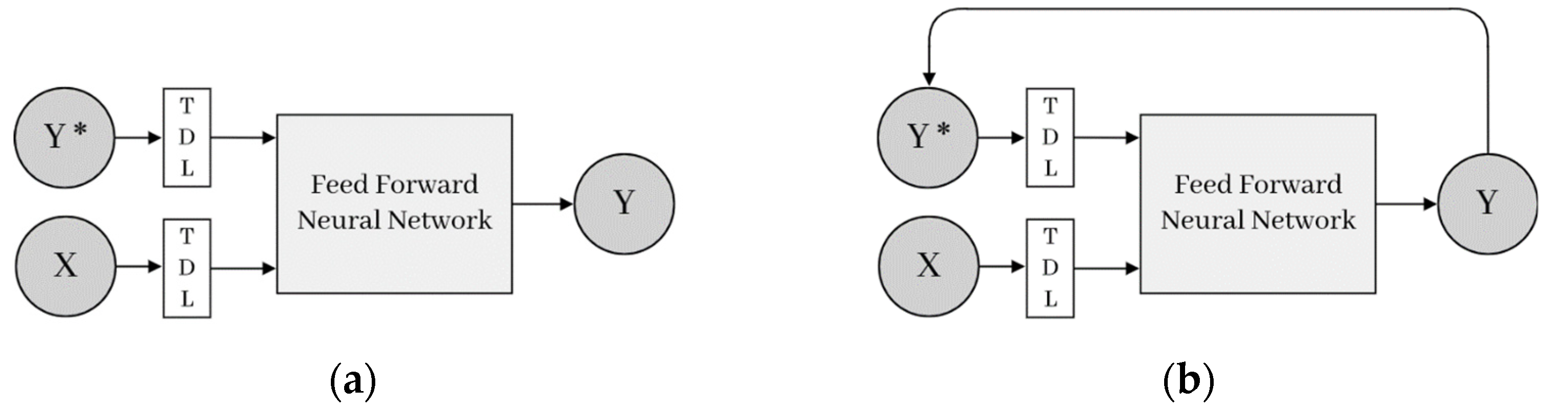
NARX neural networks are considered a type of recurrent neural network (RNN) that have been widely used in the literature for time series prediction due to, on the one hand, their easy implementation and, on the other hand, their fast-training procedures. As can be seen in
Figure 5, the predictions carried out by dynamic neural networks, such as NARX, are driven by the historical input-output pairs, as well as by the previous states of the network, that is to say, by the input and feedback delays.
In
Figure 5,
X and
Y represent the input and outputs vectors, respectively,
is the weight matrix,
is the bias, and finally, the TDL block represents the tapped-delay lines, that is to say, the number of time delay steps applied to the input and the feedback (output).
NARX neural networks are based on a Multi-Layer Perceptron (MLP) structure, which consists of an input layer, hidden layer, and output layer that are connected by adjustable weights, and the neurons that compose the hidden and output layer are associated with bias values [
24]. The weights and biases are adjusted during the training process of the network, aiming to achieve their optimal values and make the best approach between the input and output of the network.
In each layer, each neuron carries out a scalar multiplication of the input vector
and the weight matrix
Likewise, the activation function (
) is added, obtaining the following equation in the output of each neuron:
The activation function that is chosen for each layer may change depending on the application in which the neural network is used. Usually, the activation function applied in the input and hidden layer is the sigmoid, and the one used in the output layer is the linear function.
The following equation shows the input-output relationship using a NARX:
where
is the future value of the target variable,
p is the total exogenous inputs,
is the time lag of each exogenous input
and
is the time lag of the historical targeted values
.
The number of time delay steps of the output,
, is the one that gives recurrence to the NARX, in contrast to the structures of other RNNs, in which the recurrence is given by the internal state of the network [
23]. Additionally,
f is the non-linear mapping function performed by the MLP. MLP is a powerful structure very appropriate for learning any kind of nonlinear mapping [
25].
In the first place, the training of the network is performed in open-loop (series-parallel) architecture (see
Figure 6a) whenever the historical data of the targeted output are available. The network can be trained using different types of training algorithms, with the Levenberg-Marquardt backpropagation algorithm being the most widely used. After the training is concluded, the loop is closed (see
Figure 6b), and this time backs, signaled estimations are introduced to the model. In the second phase, also called simulation or operational mode, the step-ahead forecasting is carried out.
3.2.3. Support Vector Regression
SVM is a supervised machine learning method for function estimation [
26]. SVM is mostly used in classification problems but is suitable for regression tasks as well. A version of SVM for regression is referred to as SVR.
Suppose that we are given training data
, where
is the number of samples in the training set,
is an input vector, and,
is the corresponding target value. In SVR, the basic idea is to map the
into a high dimensional feature space
via a non-linear mapping function and do linear regression in this space. Thus, the linear regression in a high dimensional (feature) space corresponds to non-linear regression in a low dimensional input space [
27]. SVR approximates the regression function as follows:
where 〈
〉 denotes the dot product in
,
is a vector of weight coefficients,
is the non-linear mapping function, and
denotes the bias constant. The common formulation of SVR is Vapnik’s
-SVR.
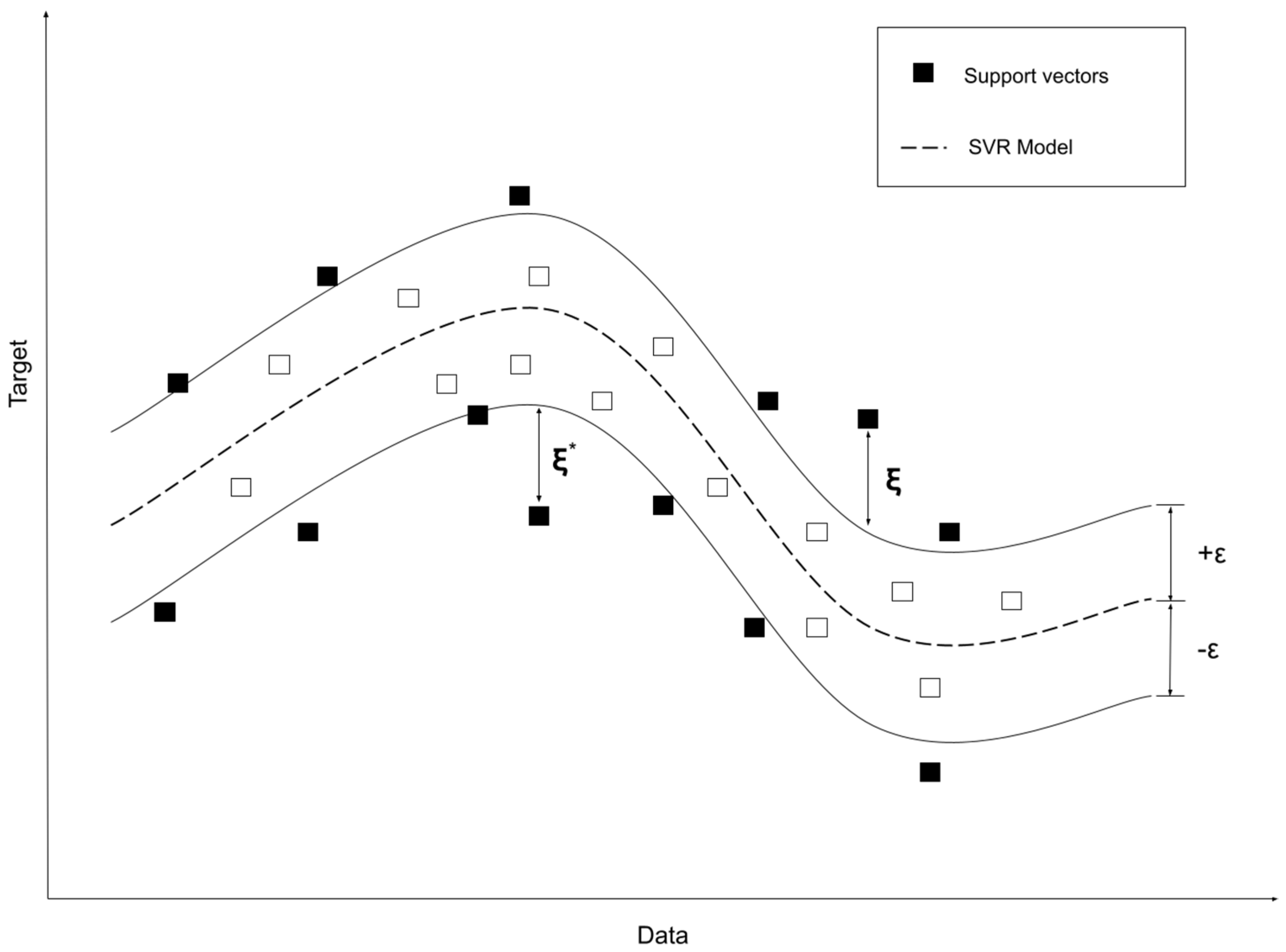
In
-SVR the goal is to find the
that has at most
deviation from the actual targets
for all the training data. We can write this problem as a convex optimization problem where the coefficients
and
can be obtained by the following formula:
where
and
are slack variables, the constant
C determines the amount up to which deviations larger than
are tolerated, and
is the margin of tolerance. This optimization problem (6) is a quadratic programming type, and in most cases, the problem can be solved more easily in its dual formulation [
28]. In the case of
-SVR the support vectors are training samples that lie on the
-tube bounding decision surface, as illustrated in
Figure 7.
As noted in the previous definitions, the algorithm only depends on dot products between vectors
. Because of this is enough to know
rather than
explicitly.
is known as the kernel function of the SVR model. The radial basis function (RBF) kernel is used in this study, expressed as:
where
defines the influence of the support vectors selected by the model.
To summarize the models, the following lines present the advantages and disadvantages of each of them.
Starting with the analytical model, as mentioned above, one of the main disadvantages of the model is that it is difficult to obtain the mathematical definition that describes the system to be modeled. For the same reason, it is necessary to have a high level of knowledge of the physical functioning of the system to be simulated. On the other hand, at the same time, by having a high level of knowledge, it is more likely that all the aspects involved in the system will be considered. Furthermore, obtaining a generic model that provides good results under different conditions.
As for the ML-type models, the main characteristic that differentiates them from the analytical model is that it is not necessary to have a detailed knowledge of the operation of the system to be modeled.
One of the major advantages of SVR is that it can obtain good results with a small dataset [
30], so it is not necessary to have a large training set. As for disadvantages, SVRs have a high dependency on hyper-parameters, and the selection of parameters determines the prediction effect of the model. Therefore, the model must be regularly adjusted to fit the characteristics of the input data to maintain a good generalization. Consequently, it requires a lot of adjustment time.
Next, the FFNN and NARX models (both ANN) have the advantage that they are very simple models, so they are very easy to implement. In addition, the NARX model presents ease of learning when the system has very large non-linearities, and it is especially efficient at predicting time-series systems. However, the vanishing and exploding gradient problem appear in the vast majority of RNNs, and NARX is no exception. This problem can be clearly seen when the information of past inputs must be recovered. Because of the vanishing problem of the gradient, the weights are less and less updated, and this causes a limitation of memory capacity. Anyway, several solutions have already been applied to avoid this problem [
23].
Finally, the FFNN model being the simplest ANN model, its design and implementation are easy since very few hyper-parameters need to be adjusted. For this reason, it is easy to obtain a general model that provides good results with little adjustment time. In contrast, it presents some difficulties when dealing with problems with large non-linearities and complex systems.
3.3. Error Metrics
In order to understand and evaluate the operation of any model, it is necessary to establish certain metrics to calculate the error of the model’s results. In this work, the developed models are assessed using three different metrics, which are widely used in the literature for accuracy evaluation purposes.
So, the models designed to forecast the day-ahead PV production curve are assessed by calculation of MAE (Mean Absolute Error), RMSE (Root Mean Square Error), and R2 (coefficient of determination).
All three metrics show great potential for comparing the operation of different models, which is of vital importance in this work.
The equations for each of them are shown below [
31].
where
and
are measured and predicted values, respectively, in this case of the PV production and
and
the mean values of both.
N represents the number of the used test samples.
With the calculation of MAE, the uniform forecast error of the model results is evaluated. The RMSE calculates the general accuracy of the model. Large deviation errors are the ones more desirable to identify, and in this case, RMSE offers robustness in dealing with this kind of error. While both mentioned metrics can range in value from 0 to infinity, the coefficient of determination, R2, takes values between 0 and 1 so that the assessment of model prediction accuracy becomes more intuitive. R2 reflects the goodness of fit of a model to the variable it seeks to explain.
5. Numeric Results and Discussion
The following section presents the results obtained with the four models developed for the prediction of PV generation. The results are presented in different ways; first, the averages of the error metrics for the month of July are shown. Then, the results are analyzed in a graphical form. Afterward, the difference in the behavior of the models depending on whether the day is sunny or cloudy is shown. Finally, the percentage errors of the models are calculated.
Table 6 shows the average of the metrics for the entire month of July. If results are analyzed in terms of the R
2 metric, the SVR model clearly stands out from the others, with a value of 0.93. Even so, it is worth mentioning that the R
2 results obtained with the other three models are actually good. Another outstanding performance is the MAE and RMSE values obtained by the analytical model, which are twice as high as those obtained with the rest of the models.
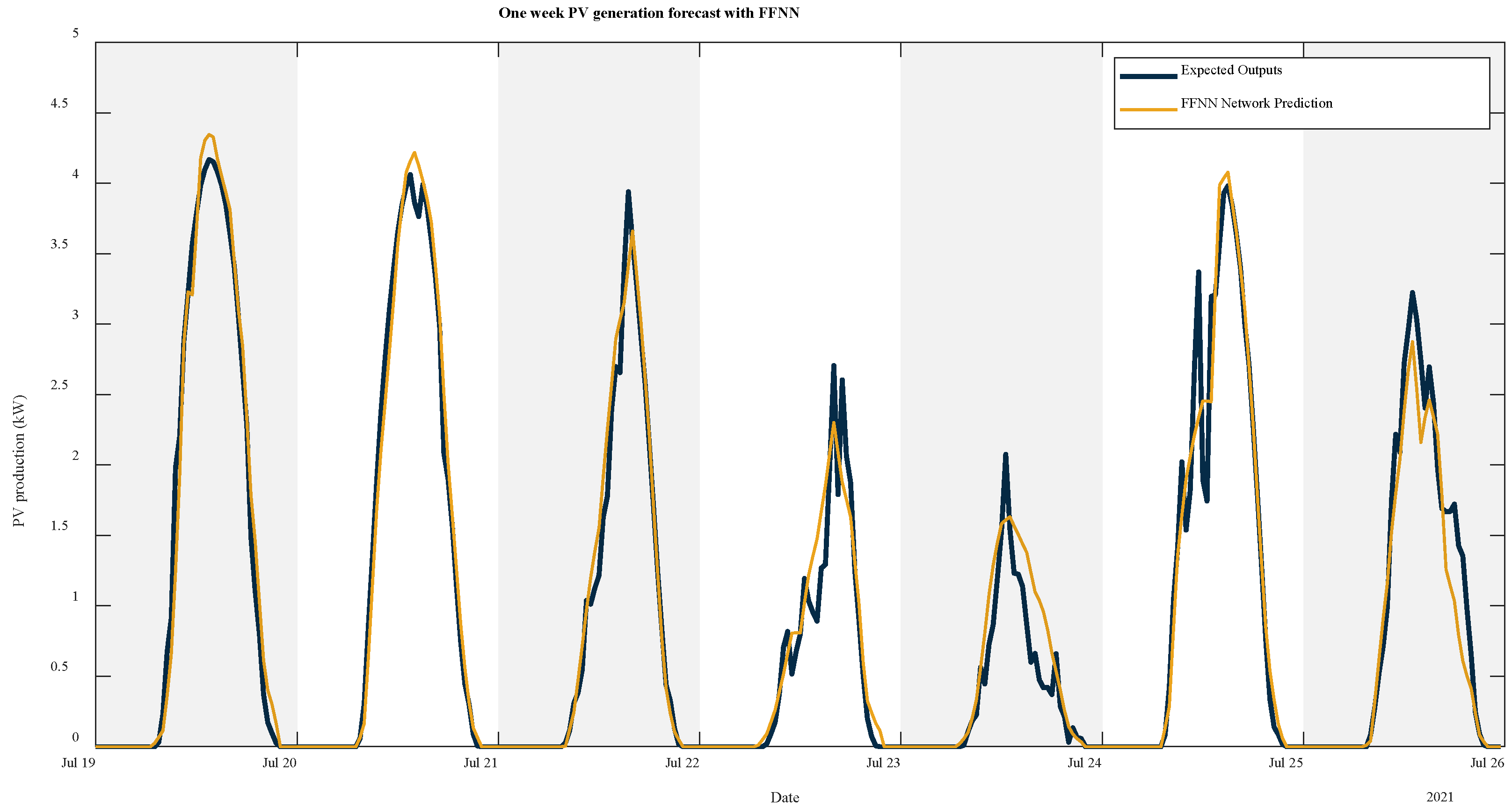
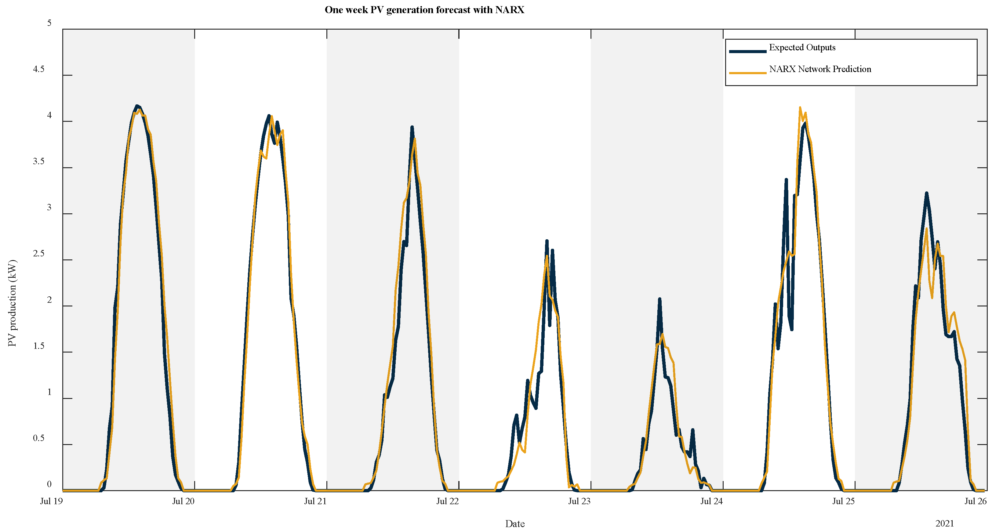
Figure 11,
Figure 12,
Figure 13 and
Figure 14 below show the predictions of PV generation during a week in July. In general, all four models are able to detect the PV generation pattern, differentiating between night and midday hours. As mentioned, all four models perform well, and this is also reflected in the figures. However, it is worth mentioning that in some aspects, models behave differently. The FFNN, NARX, and SVR models are able to reach the maximum generation peaks. Nevertheless, the FFNN model presents some complications on 22 and 23 July, which are more cloudy days. In this aspect, the SVR and NARX models show a greater ability to cope with sudden peaks. The NARX model particularly stands out on cloudy days. This model shows good behavior in dealing with constant changes. Nevertheless, it should be mentioned that at the beginning of the generation day, the NARX technique forecasts a little production when in reality, it is lower. Seeing how well the NARX model performs against cloudy days, we can conclude that its lower R
2 value compared to the others may be due to the fact that most of the days in the month of July are sunny days. Finally, the analytical model has difficulties in reaching the maximum generation peaks on each day, especially on the 23rd and 25th of July. In addition, the simulation generates a small lag in energy production. These reasons may be the explanation for the higher MAE and RMSE metrics obtained by the analytical model compared to the other models.
Afterward, continuing with the analysis of the behavior of the models according to the type of day,
Table 7 shows the R
2 values for five sunny days and five cloudy days. It is clearly noticeable that on sunny days the R
2 is around 0.95, whereas when the day is cloudy, regardless of the model, the R
2 values are around 0.8. In this case, also, the SVR model stands out for obtaining the best results.
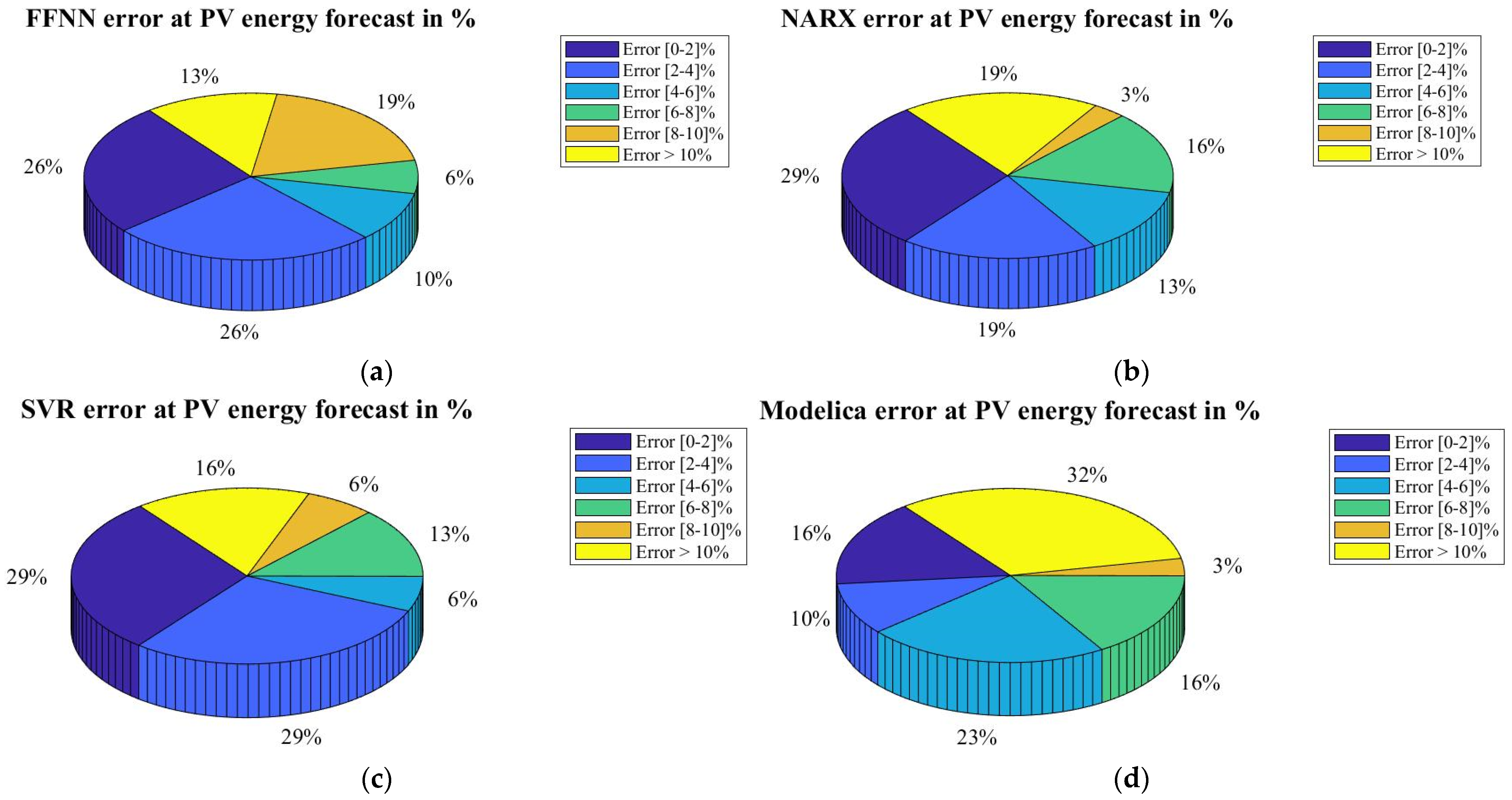
Finally, in order to analyze what happens on each day of July on a more detailed basis, the error made in the prediction of each day has been calculated. Since the results presented in
Table 6 may not be very detailed due to the fact that a punctual error of one day can ruin the average of the month. For that reason,
Figure 15 shows in a pie diagram form the daily relative error made by ranges. Summarising
Figure 15, we can see how, as on previous occasions, the SVR model stands out from the others; in 58% of the cases, it commits an error of less than 4%. In the case of the FFNN model, this occurs in 52% of the cases. In the NARX model, 48%, and, finally, with the analytical model, it is in 26% of the cases that errors of less than 4% occur. As for the maximum errors, it is the analytical model that obtains the highest errors, 32%, compared to 19%, 16%, and 13% for the NARX, FFNN, and SVR models, respectively.
Table 8 summarises the mean errors for each model.
6. Conclusions
This paper presents the development of four models to predict PV production, an analytical model developed in the open-source software OpenModelica and three AI models: an FFNN, a NARX, and an SVR. All four models are designed to predict the production of the next 24 h, with a time interval of 30 min. Predicting PV production is not an easy task due to the high dependence on solar irradiance. This work uses historically measured data to carry out the prediction.
Firstly, one of the conclusions to be highlighted is that in the framework considered, the highest prediction accuracy is obtained with the SVR model. This model obtains an average R2 of 0.934 for the July forecast. Thus, in this case, study, the SVR model performs 4.07% better than the FFNN model, 5.12% better than the NARX model, and 4.18% better than the analytical model.
Regardless of the technique used, it is concluded that forecasting on sunny days performs better than forecasting on cloudy days. This is related to the fact that PV production on sunny days is more constant, giving the characteristic bell shape of an ideal PV system production. In contrast, the forecast for cloudy days needs to cope with sudden changes.
With regard to the relative error committed on each day of July, this has been calculated in order to analyze in more detail, which is the behavior of each model for every day of the predicted month. The best performance is obtained with the model SVR, which in 58% of the cases it, commits an error of less than 4%. In comparison with the rest of the models, the SVR model performs 13.76%, 23.06%, and 83.3% better than the FFNN, NARX, and the analytical model, respectively.
Another conclusion has been drawn from the development of the different models. In terms of the development process, the analytical model requires a higher level of knowledge about how a PV installation works. Furthermore, when implementing changes in the PV installation, such as an increase in installed capacity or the degradation of the PV panels, it is more complex to implement them in the analytical model. These changes have to be manually included so that they can represent the reality of the PV installation as accurately as possible. In contrast, for AI-based models, it would only be necessary to re-train the models with the new data.
One of the changes applied in this work, compared to previous work [
34], is the use of a filter that sets the solar irradiance values between sunset and sunrise to 0. Applying this step to the pre-processing and post-processing of the data has helped to improve the behavior of the four models during the night. It should also be noted that a good pre-processing of the data is as important as the design of the model itself.
Regarding future work, a new comparison of the different models will be carried out considering predicted meteorological data instead of historical measured data. It can be thought that the predicted data, for instance, solar irradiance, will have much more influence on the results than, for example, the type of model used. Therefore, meteorological forecast data provided by different meteorological agencies will be considered, and their effect on the prediction will be analyzed. Finally, the best prediction model that uses the best meteorological forecast data will be implemented in the Izarbel EMS in order to operate in real time.


 ,
, 


