Article

A Combined Safety Monitoring Model for High Concrete Dams

1
College of Water Conservancy and Hydropower Engineering, Hohai University, Nanjing 210098, China
2
National Engineering Research Center of Water Resources Efficient Utilization and Engineering Safety, Hohai University, Nanjing 210098, China
3
Nanjing Hydraulic Research Institute, Nanjing 210029, China
4
Research Center on Levee Safety and Disaster Prevention of Ministry of Water Resources, Zhengzhou 450003, China
*
Authors to whom correspondence should be addressed.
Appl. Sci. 2022, 12(23), 12103; https://doi.org/10.3390/app122312103
Submission received: 16 October 2022 / Revised: 22 November 2022 / Accepted: 23 November 2022 / Published: 26 November 2022
(This article belongs to the Special Issue Machine Learning–Based Structural Health Monitoring)

Abstract

:
When applying reliability analysis to the monitoring of structural health, it is very important that gross errors–which affect prediction accuracy–are included within the monitoring information. An approach using gross errors identification and a dam safety monitoring model for deformation monitoring data of concrete dams is proposed in this paper. It can solve the problems of strong nonlinearity and the difficulty of identifying and eliminating gross errors in deformation monitoring data in concrete dams. This new method combines the advantages of an incremental extreme learning machine (I-ELM) method to seek an optimal network structure, the Least Median Squares (LMS) method with strong robustness to multiple failure points, the robust estimation IGG method with the good robustness to outliers (gross errors) and extreme learning machine (ELM) method with high prediction efficiency and handling of nonlinear problems. The proposed method can eliminate gross errors and be utilized to predict the behavior of concrete dams. The deformation monitoring data of an existing 305 m-high concrete arch dam is acquired by combining remote sensing technology with other monitoring methods. The LMS-IGG-ELM method is utilized to eliminate outliers from the dam monitoring sequence and is compared with the processing result from a DBSCAN clustering algorithm, Romanovsky criterion and the 3σ method. The results show that the proposed method has the highest gross errors identification rate, the strongest generalization ability and the best prediction effect.

1. Introduction

In recent years, in addition to utilizing traditional instruments for acquisition of monitoring data, comprehensive remote sensing technology has been introduced to assist measurement, so as to improve the accuracy, timeliness and reliability of the monitoring data [1,2]. The application of remote sensing technology in the field of dam safety monitoring mainly relies on the accurate calculation of the target positions by a GPS monitoring station to realize the deformation monitoring of the dam. Remote sensing technology mainly collects data from the target radiation or reflected electromagnetic waves, and the obtained image data have the advantages of large amounts of information, strong timeliness and high resolution [3]. At present, remote sensing technology has been gradually applied to civil infrastructure, mechanical equipment and other structural tests to obtain original monitoring data [4,5]. Galdelli et al. [6] utilized a remote visual inspection system to implement predictive maintenance of bridges. Shang et al. [7] proposed a new flight planning method to enable efficient data for a truss bridge reconstruction. Graves et al. [8] utilized 3D geometric measurements extracted from photogrammetric point clouds to assess the performance of highway bridges in static load testing.
The credibility of the main application of measurement results is determined by the credibility of the input data [9]. When obtaining raw data for concrete dam safety monitoring, there are often a certain number of gross errors generated from reading errors, calculation errors, the sudden failure of the detection instrument and other factors. The existence of gross errors seriously affects the accuracy of the dam observation value sequences, so effective measures must be taken to achieve a real and reliable dam safety prediction result. At present, the widely used gross errors eliminating methods include the process line method, statistical test method and mathematical model method [10,11]. However, these traditional methods have some problems such as less robustness and less comprehensive consideration. Therefore, Kim et al. [12] proposed a method for three-dimensional subsurface stratification to modify the cross-validation based on the outlier detection method. Rasheed, F [13] utilized fast Fourier transform to highlight the areas with high frequency change to identify outlier regions. Lach [14] applied several statistical test methods to detect and remove outliers in the Dobczyce dam over the period 2012–2016. Zhang et al. [15] proposed a method to identify the outliers of dam monitoring data with an abnormal index matrix updated with real-time data based on integrated learning; Song et al. [16] established a theoretical method for dam outliers monitoring based on multivariate panel data and K-mean clustering; Shao et al. [17] utilized image processing techniques and cuckoo search algorithms to process outliers in dam monitoring data. Meanwhile, scholars introduced the robust estimation theory into the model of gross errors identification, so as to enhance the robustness and generalization ability of the model. Zhao et al. [18] proposed an improved algorithm of the 3 σ method based on MCD robust estimation to identify the residual outliers in the dam detection data; Li et al. [19] established an early warning model combining robust statistics and confidence intervals to identify detection outliers; Li et al. [20] explored an improved Pauta criterion for a gross errors elimination algorithm based on M estimation, which effectively solved the problem of misjudgment of outliers; Hu et al. [21] combined the advantages of the ability of robust resistance by robust estimation and the ability of handling nonlinear problems by extreme learning machine to establish the dam safety monitoring model of M-ELM. Compared with traditional methods, these methods are able to solve the problem of outliers better in dam deformation data, but there is still misjudgment when the monitoring sequence has continuous deviation from a normal value or low deviation degree. This phenomenon should be further studied to improve the identification ability of abnormal data.
The current traditional dam safety monitoring model includes a mathematical statistical model, deterministic model and mixed model. As early as in the 1950s, Portugal, Italy and other countries began to utilize the statistical regression method to establish the dam deformation monitoring model [22,23]. In the 1970s, Chen et al. introduced statistical regression to establish the dam safety monitoring model, and explained the physical causes of the analysis results. In the mid-1980s, Wu et al. [24,25,26] established the statistical model between measured data and effect size by utilizing mathematical statistical methods such as gradual regression and weighted regression, successfully applying it in a practical project. In recent years, with the development of computers, big data and artificial intelligence, intelligent algorithms such as gray system, fuzzy mathematics, Bayes classification algorithm, chaos, wavelet theory, random forest algorithm, cluster algorithm, neural network and particle swarm optimization [27] have been introduced into the field of dam safety monitoring. Huang et al. [28] introduced nuclear partial least squares method into the safety monitoring of an ultra-high dam for the first time; Xu et al. [29] constructed a dam deformation monitoring model based on the radial basis function (RBF) neural network; Gu et al. [30] developed a monitoring factor excavation model for concrete dams based on the optimized random forest method; Gabriella et al. [31] proposed three multi-target support vector regression models, and accordingly constructed a dam deformation behavior characterization model. Alocen et al. [32] utilized stacking and blending integration strategies to predict radial movements of an arch-gravity dam.
The IGG method of selection iteration is the most commonly utilized method in robust estimation [33], and the selection of the initial value generally directly obtained through the least squares (LS). The LS-IGG method is able to accurately identify gross errors when the number of gross errors is relatively small. However, as the proportion of gross errors increases, the identification ability of this method reduces significantly, and gross errors cannot be accurately eliminated. Therefore, in this paper gross errors identification and regression analysis model is established by combining the IGG method and extreme learning machine (ELM) for gross errors identification and regression analysis of the dam detection data with the Least Median Squares (LMS) method for selecting the initial value of robust resistance estimation. The specific case is utilized to discuss the ability of gross errors identification and the effect of prediction regression of this method. Compared with the traditional gross errors identification methods, this method has a higher identification accuracy and stronger robustness; compared with traditional neural network prediction methods, it has the advantages of fast learning speed, strong generalization ability and high prediction accuracy. The proposed method is able to solve the gross errors problem effectively in the dam deformation monitoring data, and predict the dam deformation properties quickly and accurately, which will make a significant contribution to the long-term safe and healthy operation of the dam. Through the proposed intelligent algorithms in this paper, the complex nonlinear problems and numerous uncertain factors in the monitoring model could be solved more effectively, which is capable of improving the robustness and generalization ability of the dam safety monitoring model and the prediction accuracy of the dam safety monitoring [34].

2. Method

2.1. Method of Acquiring the Data with the GPS Technique

In order to effectively acquire the monitoring data of dam deformation, the reference points, working basis points and deformation observation points are selected according to the “GPS standard”, and this three-level monitoring network is set up. The layout requirements are exhibited in Table 1. During automated monitoring, the observation points receive GPS signals in real time, and send the data to the control center through the communication network, as exhibited in Figure 1. The control center is able to utilize the corresponding software to calculate the three-dimensional coordinates of each monitoring point in real time, so as to obtain the deformation of the dam.

2.2. The Gross Errors Detection Method of Concrete Dam Deformation Monitoring Data Based on IGG-ELM

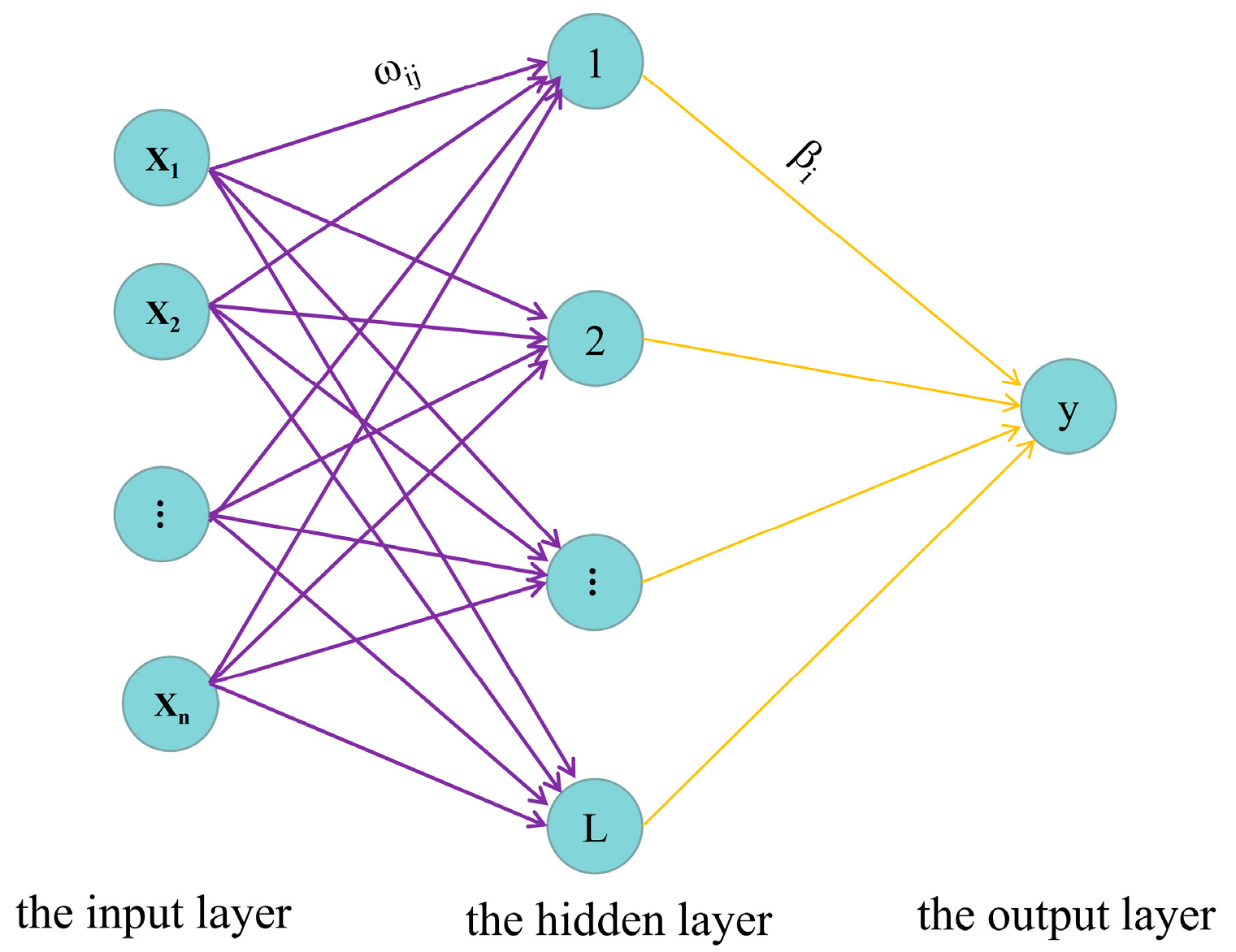
ELM is a simple and efficient feedforward neural network with a single hidden layer, of which neural network structure is exhibited in Figure 2. The parameters in Figure 2 indicate respectively:
W = [ ω 11 ω 12 ω 1 n ω 21 ω 22 ω 2 n ω l 1 ω l 2 ω ln ] β = [ β 1 β 2 β l ] b = [ b 1 b 2 b l ]
where W is the connection weight between the input and the hidden layer, β is the connection weight between the hidden and the output layer, b is the random bias of the hidden layer. Compared with traditional neural network algorithms (such as back propagation algorithm), it is not necessary to adjust the weight of each layer and the threshold of the hidden layer after the prediction of deviation in ELM. Instead, the connection weights between the input layer and the hidden layer and the bias of the hidden layer of the neural network are randomly generated. Then, through the solution of the equation group, the connection weights between the hidden layer and the output layer are found. Therefore, compared with traditional neural network algorithms, ELM has the advantages of fast learning speed, strong generalization ability, and high prediction accuracy [35,36,37].
The Least Squares (LS) method is a classical estimate utilized in ELM, which gives the same weight to all monitoring data. However, this method will be affected intensively when numbers of outliers exist in the actual measured data. Therefore, we introduce the IGG method as a robust estimation for ELM. According to the size of the residual differences between training samples and actual measurement, the weight of outliers is gradually reduced through selection weight iteration, and finally achieves elimination of the outliers.
The main influential factors of concrete dam deformation and measured data are composed of set { ( x j , t j ) } . If there are Q different monitoring samples available, the set indicates as { ( x j , t j ) } j = 1 Q , where x j = [ x 1 j , x 2 j , , x n j ] T R n , j [ 1 , Q ] is the main influence factor of the concrete dam deformation, which is regarded as the network input vector; t j is the measured deformation value of the concrete dam, which is regarded as the network desired output vector. For the ELM output model containing L hidden layer nodes:
T = [ t 1 , t 2 , , t Q ]
y j = i = 1 l β i g ( ω i x j + b i ) , j = 1 , 2 , , Q
where y j represents the corresponding output vector for the input x j in the ELM model, g ( ω i x j + b i ) represents the corresponding activation function for the input x j in the ELM model, g ( ω i x j + b i ) represents the corresponding activation function for the input x j vector, in this paper the “Sigmoid” type activation function is utilized, of which expression is:
g ( ω i x j + b i ) = 1 1 + e ( ω i x j + b i )
where ω i = [ ω i 1 ω i 2 ω i n ] , x j = [ x 1 j x 2 j x n j ] T .
The traditional ELM output weight β i utilizing LS to construct loss function:
Q = i = 1 Q   ( t i y i ) 2
When Q obtains the minimum value, according to Equations (1) and (2) it can be approximated as: H β = T , and the output weight of the hidden layer node of the neural network can be calculated:
β = H + T = ( H T H ) 1 H T T
In equation:
H ( ω 1 , ω 2 , , ω l , b 1 , b 2 , , b l , x 1 , x 2 , , x Q ) =
[ g ( ω 1 x 1 + b 1 ) g ( ω 2 x 1 + b 2 ) g ( ω l x 1 + b l ) g ( ω 1 x 2 + b 1 ) g ( ω 2 x 2 + b 2 ) g ( ω l x 2 + b l ) g ( ω 1 x Q + b 1 ) g ( ω 2 x Q + b 2 ) g ( ω l x Q + b l ) ] , H + is the M o o r e P e n r o s e Generalized Inverses of the output matrix for the hidden layer; T is the transposition of the Matrix T .
The mathematical model expression of applying robust estimation into the ELM is:
H β + e = T
where e is a residual vector, and the error of the i sample is expressed as:
e i = t i j = 1 L h i j β j
The structural loss function is expressed as:
Q = i = 1 Q ρ 2 ( e i ) = i = 1 Q ρ 2 ( t i j = 1 L h i j β j )
where ρ ( ) is the influence function, Q is the total number of samples. Let ψ ( e i ) = ρ ( e i ) ( e i ) , the condition of optimal solution between the connection weight β of the hidden layer and the output layer is Q getting the minimum, then: ρ ( e i ) ( β j ) = 2 ψ ( e i ) h i = 0 , then it is expressed as:
i = 1 Q ψ ( e i ) h i = 0
Let ψ ( e i ) = b i e i , where b i represents weight factor, then: i = 1 Q b i e i h i = 0 , rewrite to the matrix form:
H T B ( T H β ) = 0
Then:
β = ( H T B H ) 1 H T B T
Due to the weights of the actual deformation of the dam are P i , let P = { P i } = { P i b i } , and the matrix of the normal equations is expressed as:
β = ( H T P H ) 1 H T P T
The selection iteration method in the robust estimation is to determine the weight factor according to the residue size, among which the most effective robust scheme is to utilize the IGG method to gradually reduce the weight of the abnormal value to accurately identify the outliers [38]. The IGG equivalent weight function is expressed as:
P i = { 1 k 1 σ | e i | 0 | e i | < k 1 σ k 1 σ | e i | < k 2 σ | e i | k 2 σ
where, k 1 = 1.5 , k 2 = 2.5 ; σ expresses the observation error. The treatment method is exhibited in Table 2:

2.3. Determine the Principle of Initial Value in Selection Iteration Based on the LMS Method

According to the data [39], whether the LS resistance estimates collapsed is directly related to the number of outliers. The IGG-ELM method can accurately identify the abnormal value when the number of outliers is small, but the performance of resistance ability becomes poorer when the number of outliers increases dramatically. Therefore, the Least Median Squares (LMS) method is chosen to substitute for the traditional LS method in this paper to determine the initial value in selection iteration.
The main principle of LMS is to minimize the median squared residue of the sample sequence. If you select n from the Q observation equations, calculate the parameter x, together with group C Q n solution, the median of the residual square in the i group is:
m e d [ v i 2 ] = m e d i a n [ v i 1 2 v i 2 2 v i n 2 ] T
where i = 1 , 2 , , Q , and m e d i a n is the median operator, then:
v m e d = min ( m e d ( v 1 2 ) m e d ( v 2 2 ) m e d ( v Q 2 ) )
The unit weighted variance expresses as:
σ = 1.4826 v m e d
This value is estimated as the initial value in the Equation (13).

2.4. Determine the Number of Hidden Layer Nodes through the Incremental Extreme Learning Machine Method (I-ELM)

Suppose the initial number of nodes in the ELM network structure is s 1 , then β s 1 = ( H s 1 T H s 1 ) 1 H s 1 T T , when a new node is added in it, the connection weight between the hidden layer and the output layer is β s = ( H s T H s ) 1 H s T T , where H s = [ H s 1 , v s ] , v s is the hidden layer output vector connected to s hidden layer node.
Let D s 1 = ( H s 1 T H s 1 ) 1 H s 1 T , D s = ( H s T H s ) 1 H s T , then ( H s T H s ) 1 = ( [ H s 1 T v s T ] [ H s 1 v s ] ) 1 = [ H s 1 T H s 1 H s 1 T v s v s T H s 1 v s T v s ] 1 .
Due to ( H s T H s ) 1 is symmetrical, therefore:
( H s T H s ) 1 = [ A B B E ] 1 = [ A B B T E ]
In equation:
{ A = H s 1 T H s 1 B = H s 1 T v s C = v s T v s
There is:
I = [ A B B T E ] [ A B B T E ] = [ A A + B B T A B + B E B T A + E B T B T B + E E ]
The solution is:
{ A = A 1 B ( A 1 B ) T E B T ( A 1 B ) + A 1 B = A 1 B B T A 1 B E C = 1 E B T A 1 B
Therefore, Ds is expressed as:
D s = [ A B B T E ] [ H s 1 T v s T ] = [ A H s 1 T + B v s T B T H s 1 T + E v s T ]
Let D s = [ M N ] , input Equations (18) and (20) into Equation (21), then M , N and β s are calculated.

2.5. Specific Steps of Eliminating Gross Errors of the Dam Monitoring Data

For a given data-fit segment N = { ( x i , t i ) | x ( 1 , n ) , i ( 1 , Q ) } , the initial number of the hidden level nodes is s , the maximum number of hidden layer nodes is s max , the expected accuracy is ε .
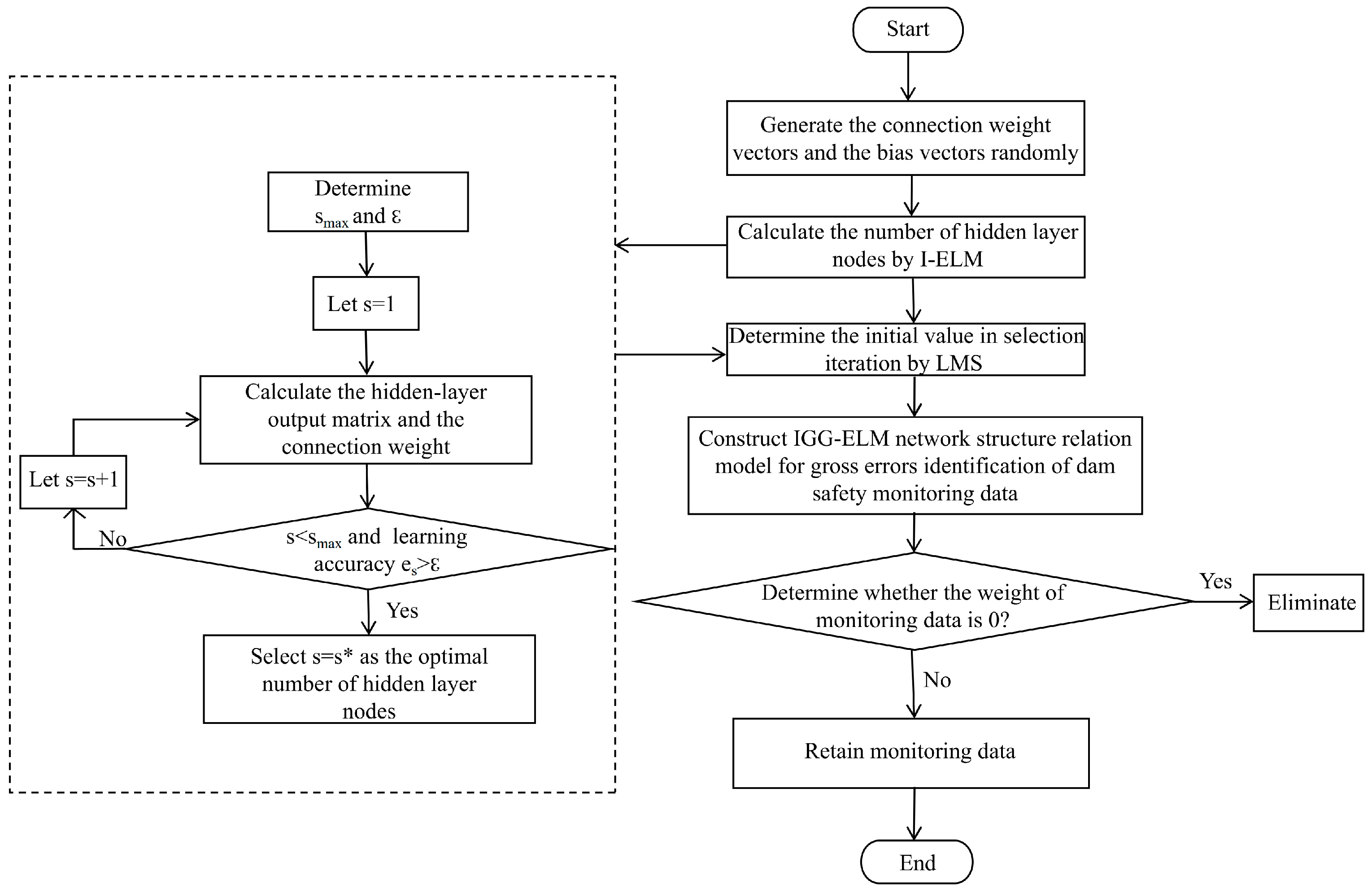
Step 1: The dam environment factors connection weight vectors ω i between the input layer and the hidden layer and the bias vectors b i of the hidden layer are randomly generated in the ELM network structure ( i = 1 , 2 , , s ) ;
Step 2: Let s = 1 , calculate the hidden-layer output matrix H 0 and the connection weight of fitting effector factor of concrete dam β 0 between the hidden layer and the output layer, and calculate learning accuracy e s = e 0 ;
Step 3: Let s = s + 1 , calculate the output matrix H s = [ H s 1 , v s ] and the connection weight of fitting effector factor of concrete dam β s until s s max or e s < ε , the optimal number of hidden layer nodes s * is obtained;
Step 4: Utilize the LMS method to calculate the unit weighted variance of deformation monitoring data of concrete dam σ , then the initial equivalence weight matrix P is also obtained;
Step 5: According to H s * in Step 3 and P in Step 4, use Equation (12) to calculate β ;
Step 6: Calculate by iteration successively until | β i + 1 β i | δ stopped;
Step 7: Output the monitoring deformation weight of concrete dam in the continuous time series P i , the sample series of P i to 0 are judged as gross errors and eliminated.
The flow of gross errors identification by LMS-IGG-ELM is shown in Figure 3:

3. Case Study

3.1. Project Overview

A hydropower station is located in Yanyuan and Muli counties, in the Liangshan Yi nationality autonomous prefecture, Sichuan Province, which is the ladder rolling development leading reservoir power station of the main stream of the Yalong River (see Figure 4). The normal storage level of the reservoir is 1880.0 m, dead water level is 1800.0 m, and the main task of the reservoir is to generate electricity, including flood control and sand control. The main building of the hydropower station is a concrete double-curved arch dam whose crest elevation is 1885.0 m and the maximum dam height is 305.0 m. In this paper the displacement monitoring data are selected from 1 September 2016 to 19 May 2018 of this hydropower dam station operation period as a case to analyze and verify the accuracy and applicability of the method utilized.

3.2. Selection of Model Influence Factors and Division of Data Sets

In the process of concrete dam operation, the dam is subject to a combination of water pressure, uplift pressure, sediment pressure and temperature load. The water pressure component ( δ H ), temperature component ( δ T ) and aging component ( δ θ ) are selected as independent variables, and the displacement vector of the dam deformation ( δ ) is selected as a dependent variable. ELM is utilized to establish the nonlinear mapping between independent variables and dependent variables, which can better construct the prediction model of dam deformation displacement. Its expression is as follows:
δ = δ H + δ T + δ θ
In Equation (22), H H 0 ,   H 2 H 0 2 ,   H 3 H 0 3 ,   H 4 H 0 4 are selected as water pressure factors, sin 2 π t 365 sin 2 π t 0 365 , cos 2 π t 365 cos 2 π t 0 365 , sin 4 π t 365 sin 4 π t 0 365 , cos 4 π t 365 cos 4 π t 0 365 are selected as temperature factors, θ θ 0 ,   ln θ ln θ 0 are selected as aging factors, where θ = 0.01 t , θ 0 = 0.01 t 0 .
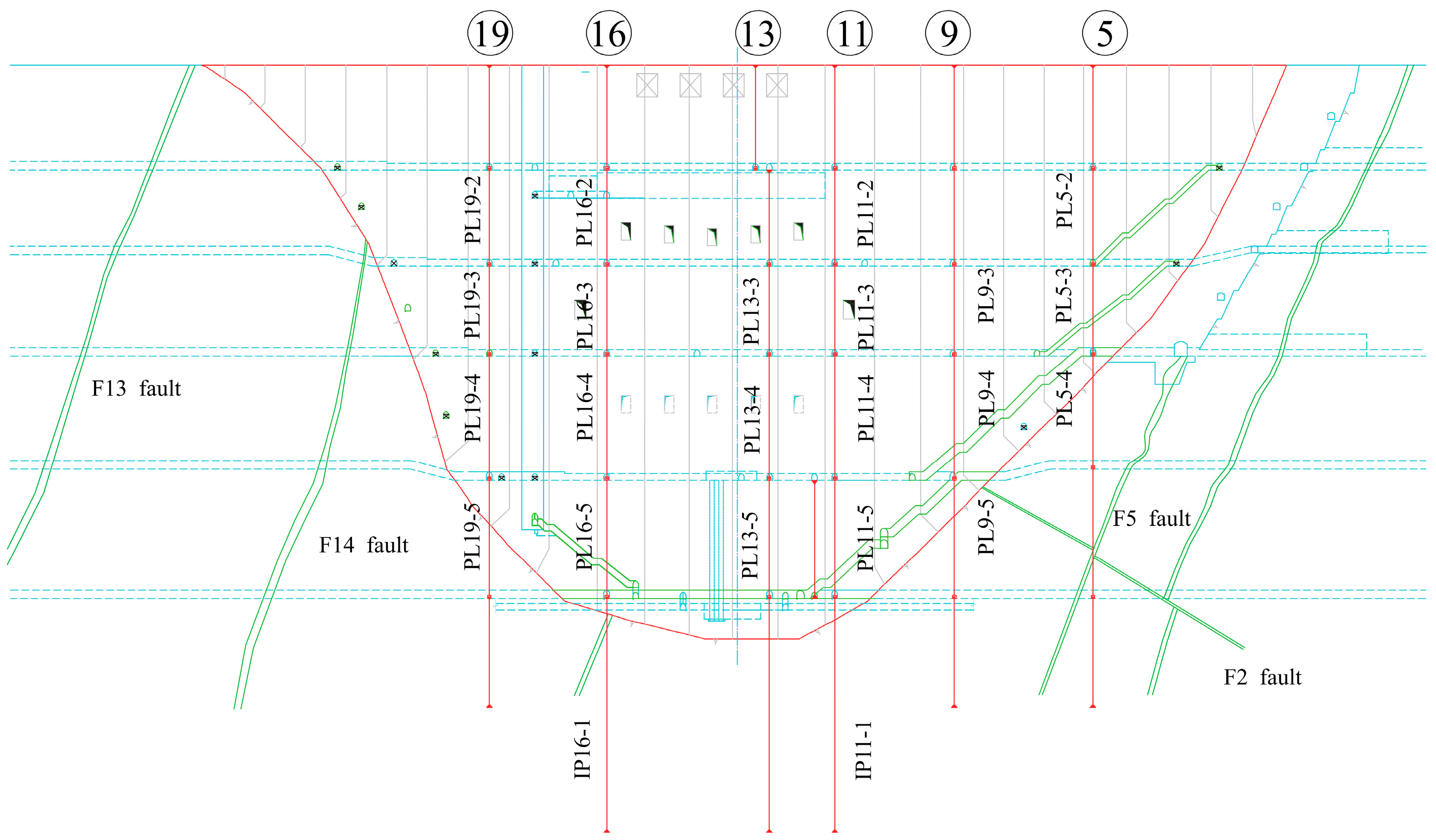
The GPS deformation monitoring system, combined with other monitoring methods, is used to obtain the monitoring data on the radial displacement of the dam, as shown in Figure 5. Multiple groups of vertical lines are arranged for the dam and dam foundation, including one group arranged for the dam foundation on both sides, one group arranged for the cushion block of the left bank, one group arranged for 5# dam section, 9# dam section, 11# dam section, 13# dam section, 16# dam section and 19# dam section each, and each group includes the normal and inverted plumb line method. The GPS measuring point is mainly set at the dam crest, corresponding to the position of plumb lines.
The monitoring data of the crown cantilever arch dam are critical for the deformation safety of the arch dam, therefore PL13-3 of the monitoring point in Figure 5 is selected as the research object. The radial displacement monitoring data are divided into a fitting segment (data samples used for model fitting) and a validation segment (data samples used to verify the generalization capability of the model), from 1 September 2016 to 22 March 2018 (522 in total) and from 23 March 2018 to 19 May 2018 (58 in total).
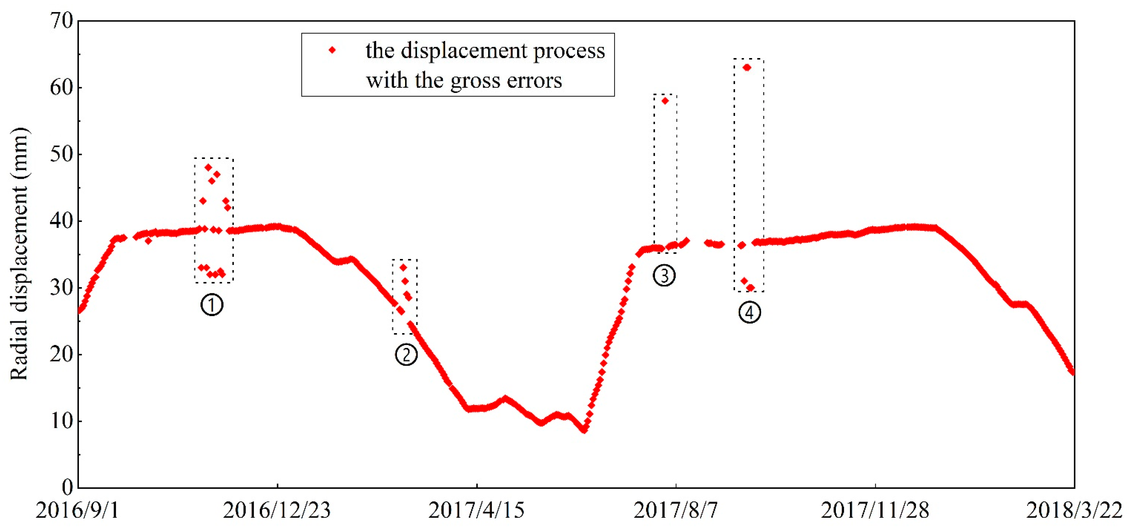
In order to test the effect of LMS-IGG-ELM method in identifying the gross errors, four types of gross errors of shock, ridge platform, jump and step are introduced into PL13-3 (the gross errors types are respectively counted as ①, ②, ③, ④). The displacement process line of the measurement point is exhibited in Figure 6.
Firstly, ω i and b i are generated randomly in the ELM network structure, and the number of hidden layer nodes is initialized to one, and the fitting segment data is processed as Equation (22) before inputting into the network structure. Secondly, the number of hidden layer nodes s is constantly increased, when s = 42 , the required learning accuracy is met, therefore the number of nodes of the hidden layer is selected to 42. Thirdly, for δ = 0.001 , selection iteration is performed utilizing the LMS-IGG-ELM method, and the weights are calculated for each fitting segment data. The first and last iteration weights of the inserted gross errors in Figure 6 are exhibited in Table 3, and all the outliers of the data for the fitting segment are identified based on the final iteration weights.

3.3. Comparison and Analysis of the Gross Error Removal Effect

In this paper, the LMS-IGG-ELM gross errors identification method is utilized to compare with the popular DBSCAN clustering algorithm, the traditional Romanovsky criterion and the 3 σ method to verify and analyze the effects of different methods, which are exhibited in Table 4 and Table 5:
Where N d is the number of gross errors identified, and r d ( % ) is expressed as:
r d ( % ) = N d t o t a l g r o s s e r r o r s × 100 %
From Table 4 and Table 5, using the traditional 3 σ method and Romanovsky criterion can only identify extremely obvious gross errors, so the identification ability of the gross errors is poor; using the DBSCAN clustering algorithm can identify 16 gross errors, the identification rate is 72.73%; using the LMS-IGG-ELM method can identify 22 gross errors with an identification rate of 100%. We adjusted the size values of these gross errors, conducted five sets of experiments, and the resulting gross errors identification effect was basically consistent, which verified the generalization and reliability of the method. Through comparison, the LMS-IGG-ELM method has better resistance to gross errors, which can accurately identify the outliers in the dam displacement monitoring data and eliminate them; meanwhile, the parameters ω and b in the ELM are randomly generated, which overcomes the time complexity by avoiding repeated adjustment parameters and significantly improves the identification efficiency of gross errors.

3.4. Validation Effect after Eliminating Gross Errors

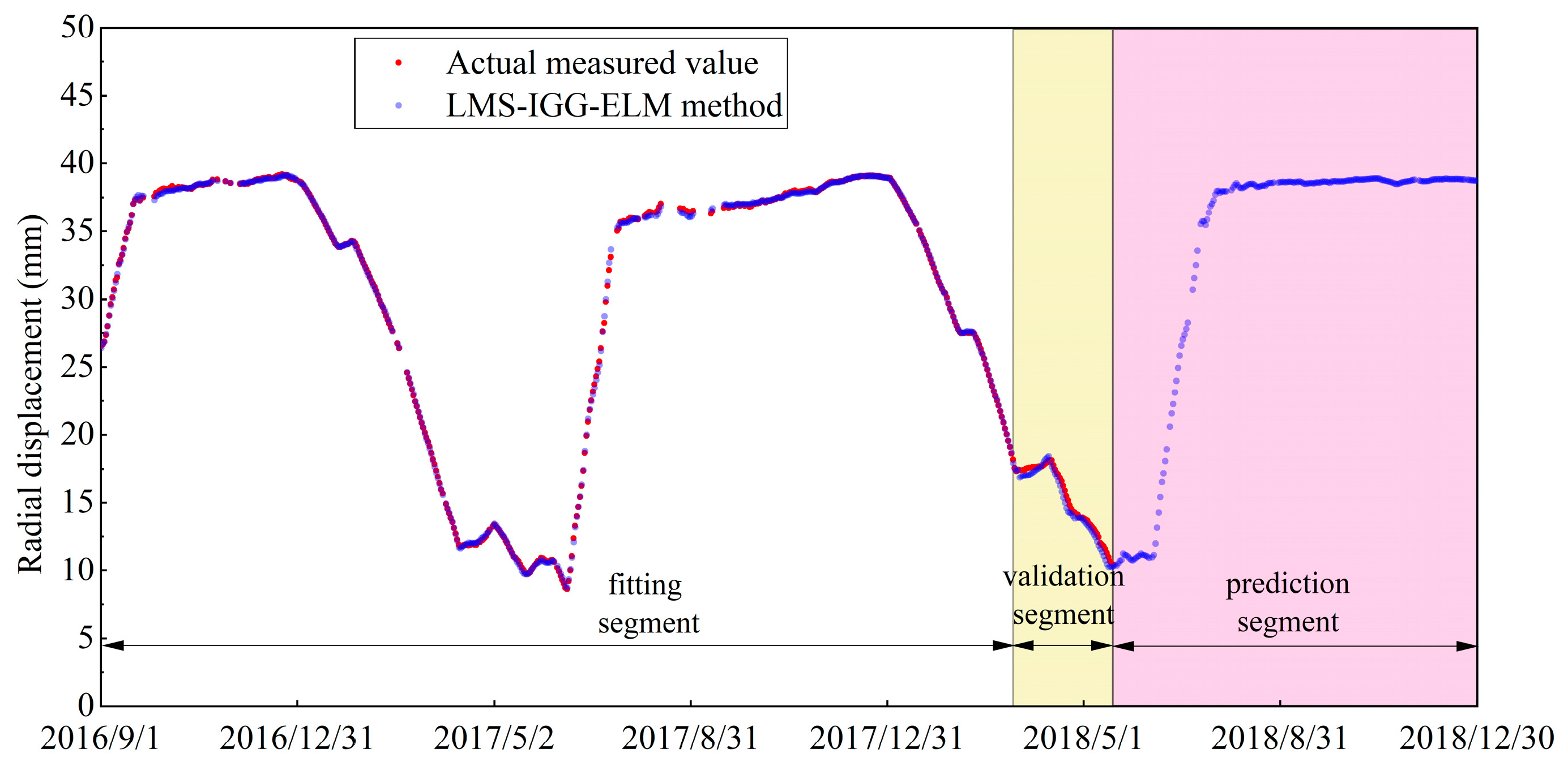
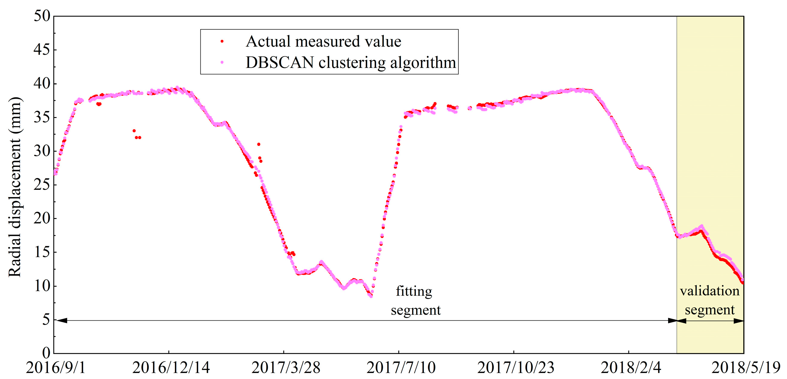
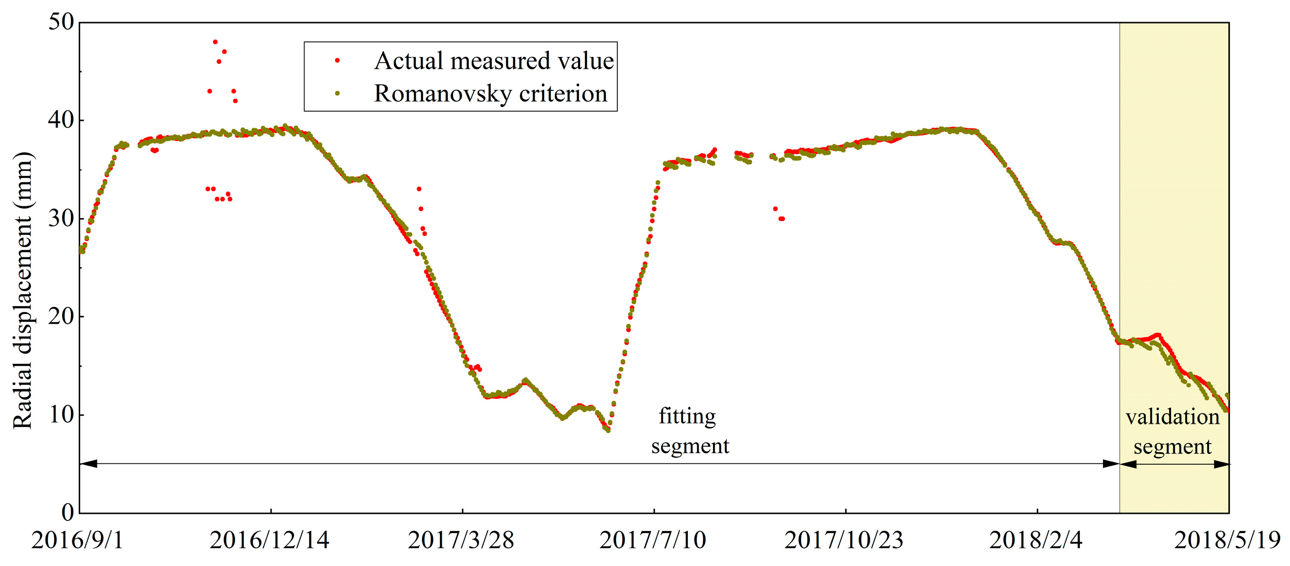
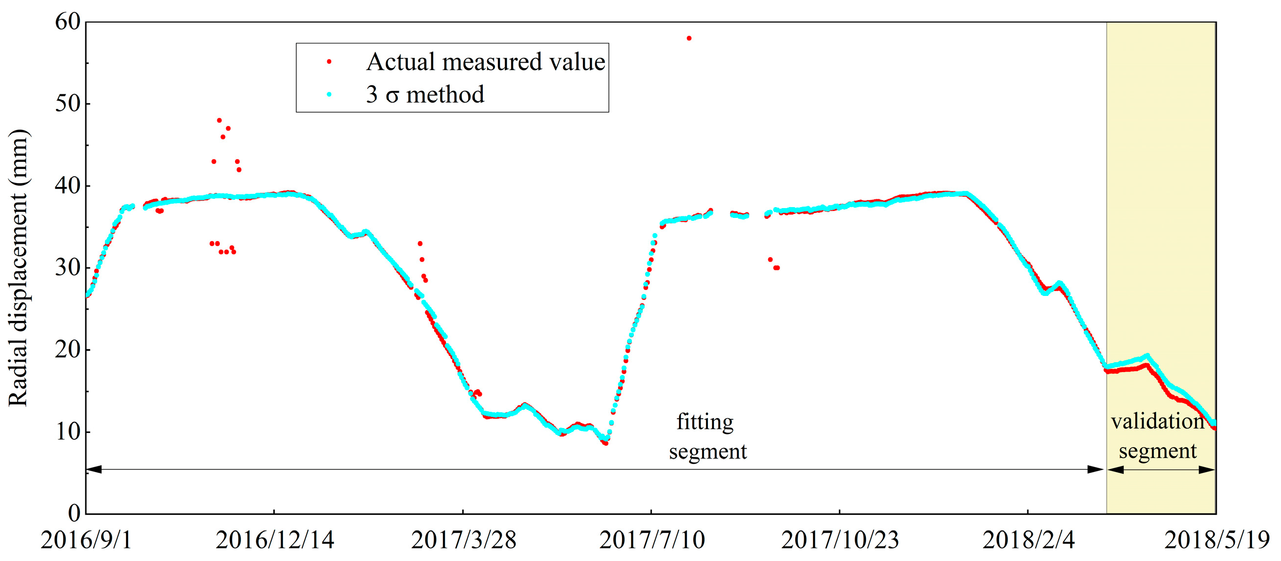
According to the data in Table 4, utilizing the LMS-IGG-ELM method to establish the dam safety monitoring model after eliminating outliers for the four methods, and making a prediction according to water pressure, temperature and aging component from 21 May 2018 to 30 December 2018, proves the final generalization ability of the model (see Figure 7, Figure 8, Figure 9, Figure 10 and Figure 11). It can be seen from Figure 7, after eliminating outliers by using the LMS-IGG-ELM method, the fit values of the model basically coincide with the actual measured values in the fitting and validation segment, so the fitting effect is quite good; and it can be seen from the scatter arrangement of the predicting segment that the change trend of dam radial displacement follows the change law of the fitting segment, which indicates that the method has good prediction accuracy and good generalization ability.
Mean absolute error (MAE), root mean square error (RMSE) and coefficient of determination (R2) are selected as evaluation indicators for comparison, which are defined as follows and are shown in Table 6, thus verifying the influence of gross errors identification effect on the accuracy of subsequent dam safety monitoring.
M A E = i = 1 n | y i y i | n
R M S E = i = 1 n ( y i y i ) 2 n
R 2 = i = 1 n ( y i y i ) 2 i = 1 n ( y i y i ) 2 = 1 i = 1 n ( y i y i ) 2 i = 1 n ( y i y i ) 2
In the equation y i represents the average of the dam monitoring data, y i represents the result of the model fitting, y i represents actual measured values of dam deformation and n represents the number of deformation monitoring data points.
It can be seen from Table 6, in the dam radial displacement verification after eliminating outliers, R2 for all four methods is above 0.85, and MAE and RMSE of the validation segment are all below 1, which indicates that the LMS-IGG-ELM method is reasonable and accurate. MAE, RMSE, and R2 of the fitting segment and validation segment after eliminating gross errors by the LMS-IGG-ELM method are 0.0890, 0.1261, 0.9998 and 0.3284, 0.4101, 0.9720, which are the set of data with the smallest errors and the strongest correlation among the four methods. In conclusion, we show that the LMS-IGG-ELM method eliminates the highest proportion of gross errors, and the monitoring effect of the subsequent dam radial displacement is also the best.

4. Conclusions

In the raw data of dam safety monitoring, the existence of gross errors will seriously affect the accuracy of the dam safety evaluation results. This paper proposes a novel method to efficiently identify outliers and predict the behavior of concrete dams, combined with the Least Median Squares method, the robust estimation IGG method and extreme learning machine method. The main contents are as follows:
(1) In view of the gross errors problem in the dam safety monitoring data under the influence of complicated factors, this paper proposes a novel method to eliminate gross errors, which combines the advantages of the Least Median Squares method with strong robustness to multiple failure points, the robust estimation IGG method with the good robustness to outliers and extreme learning machine with strong generalization ability and fast operation speed when processing sample data.
(2) Through the case study, the deformation monitoring data of a 305.0 m hyperbolic arch dam arch crown beam is utilized and compared with three other methods to verify the superiority of LMS-IGG-ELM method in eliminating gross errors. In the dam monitoring data sequences with 22 gross errors, the proposed method has an outlier identification rate of 100%, which is much higher than the traditional outlier identification method.
(3) Meanwhile, the proposed method also enables the prediction of the dam’s behavior. The dam safety monitoring model of LMS-IGG-ELM is utilized after eliminating gross errors by the four methods to verify that the proposed method has the best fitting effect and the highest prediction accuracy. LMS-IGG-ELM method is able to solve the problem of outlier identification in continuous time series data well, and can be applied widely to other projects such as roads and bridges.

Author Contributions

Conceptualization, Y.W., H.G. and C.G.; methodology, Y.W.; software, Y.W.; validation, Y.W., H.G., M.Y., W.C., Z.F. and Y.H.; formal analysis, Y.W.; investigation, Y.W.; resources, Y.W.; data curation, Y.W.; writing—original draft preparation, Y.W.; writing—review and editing, Y.W. and H.G.; visualization, Y.W.; supervision, H.G. and Y.H.; project administration, Y.W.; funding acquisition, H.G. and C.G. All authors have read and agreed to the published version of the manuscript.

Funding

This work was supported by the key projects supported by the Joint Fund of the National Natural Science Foundation of China (Grant No. U2243223, 51739008); the National Natural Science Foundation for Young Scientists of China (Grant No. 51909173); Water Conservancy Science and Technology Project of Jiangsu (Grant No. 2022024); State Key Program of National Natural Science of China (Grant No. 51739003); China Postdoctoral Science Foundation (Grant No. 2021M701044, 2022M721668), Open fund of National Dam Safety Research Center (Grant No. CX2020B02); Open Fund of Research Center on Levee Safety Disaster Prevention of Ministry of Water Resources under Grant LSDP202204; Jiangsu Young Science and Technological Talents Support Project TJ-2022-076. Open fund of Research Center on Levee Safety and Disaster Prevention of Ministry of Water Resources (Grant No. LSDP202204).

Institutional Review Board Statement

Not applicable.

Informed Consent Statement

Not applicable.

Data Availability Statement

Not applicable.

Conflicts of Interest

The authors declare no conflict of interest.

References

  1. Ding, Y. Improvement of Dam Deformation Monitoring System by Remote Sensing Technology. J. Silicon Val. 2013, 5, 217–218. [Google Scholar]
  2. Yang, G. Application of GPS combined with near-view photography in landslide monitoring. J. Tour. Overv. 2011, 12, 66. [Google Scholar]
  3. Song, W.; Lv, J.; Liu, C.; Yang, L.; Huang, H.; Liu, Y.; Shi, Z.; Yan, S.; Lv, G.; Li, X. The Application of Remote Sensing Technology in the Construction of Digital Twin Watershed. J. China Flood Control. Drought Relief 2022, 32, 15–20. [Google Scholar]
  4. Luo, W. Application of GPS in Deformation Monitoring of Hydropower Station. J. Value Eng. 2022, 41, 129–131. [Google Scholar]
  5. Xi, R.; Liang, Y.; Chen, Q.; Jiang, W.; Chen, Y.; Liu, S. Analysis of Annual Deformation Characteristics of Xilongchi Dam Using Historical GPS Observations. Remote Sens. 2022, 14, 4018. [Google Scholar] [CrossRef]
  6. Galdelli, A. A Novel Remote Visual Inspection System for Bridge Predictive Maintenance. Remote Sens. 2022, 14, 2248. [Google Scholar] [CrossRef]
  7. Shang, Z.; Shen, Z. Flight Planning for Survey-Grade 3D Reconstruction of Truss Bridges. Remote Sens. 2022, 14, 3200. [Google Scholar] [CrossRef]
  8. Graves, W.; Aminfar, K.; Lattanzi, D. Full-Scale Highway Bridge Deformation Tracking via Photogrammetry and Remote Sensing. Remote Sens. 2022, 14, 2767. [Google Scholar] [CrossRef]
  9. Gabbar, H.A.; Chahid, A.; Alam Khan, J.; Adegboro, O.G.; Samson, M.I. CTIMS: Automated Defect Detection Framework Using Computed Tomography. Appl. Sci. 2022, 12, 2175. [Google Scholar] [CrossRef]
  10. Li, X.; Jiang, M.; Wu, Z.; Chen, J. Comparison and improvement of coarse difference identification methods in dam safety monitoring data. J. Rural Water Resour. Hydropower China 2011, 3, 102–105+112. [Google Scholar]
  11. Gu, H.; Yang, M.; Gu, C.; Huang, X. AC-IBFGS-Based Inversion Method for Estimating the Quasi-Viscoelastic Parameters of Arch Dams. IEEE Access 2022, 10, 68151–68160. [Google Scholar] [CrossRef]
  12. Kim, H.S.; Chung, C.K.; Kim, H.K. Geo-spatial data integration for subsurface stratification of dam site with outlier analyses. Environ. Earth Sci. 2016, 75, 1–10. [Google Scholar] [CrossRef]
  13. Rasheed, F.; Peng, P.; Alhajj, R.; Rokne, J. Fourier Transform Based Spatial Outlier Mining. Lect. Notes Comput. Sci. 2009, 5788, 317–324. [Google Scholar]
  14. Lach, S. The application of selected statistical tests in the detection and removal of outliers in water engineering data based on the example of piezometric measurements at the Dobczyce dam over the period 2012–2016. E3S Web Conf. 2018, 45, 4500045. [Google Scholar] [CrossRef]
  15. Zhang, J.; Xie, J.; Kou, P. Abnormal Diagnosis of Dam Safety Monitoring Data Based on Ensemble Learning. J. IOP Conf. Ser. Earth Environ. Sci. 2019, 267, 062027. [Google Scholar]
  16. Song, J.; Zhang, S.; Tong, F.; Yang, J.; Zeng, Z.; Yuan, S. Outlier Detection Based on Multivariable Panel Data and K-Means Clustering for Dam Deformation Monitoring Data. J. Adv. Civ. Eng. 2021, 2021, 3739551. [Google Scholar] [CrossRef]
  17. Shao, C.; Zheng, S.; Gu, C.; Hu, Y.; Qin, X. A novel outlier detection method for monitoring data in dam engineering. J. Expert Syst. Appl. 2022, 193, 116476. [Google Scholar] [CrossRef]
  18. Zhao, Z.; Chen, J.; Zhang, H.; Li, Y.; Wu, Z. Crude difference identification method for dam monitoring data based on robust estimation. J. Hydropower Energy Sci. 2018, 36, 68–71. [Google Scholar]
  19. Li, X.; Li, Y.; Lu, X.; Wang, Y.; Zhang, H.; Zhang, P. An online anomaly recognition and early warning model for dam safety monitoring data. J. Struct. Health Monit. Int. J. 2020, 19, 796–809. [Google Scholar] [CrossRef]
  20. Li, X.; Li, Y.; Zhang, P.; Yang, Z. Research and application of an improved Pauta criterion based on M estimation in coarse difference identification of monitoring data. J. China’s Rural Water Resour. Hydropower 2019, 8, 133–136. [Google Scholar]
  21. Hu, D.; Qu, X.; Yang, J.; Cheng, L.; Chang, M. The Dam Deformation Safety Monitoring Model Based on M-ELM. J. Prog. Water Conserv. Hydropower Technol. 2019, 39, 75–80. [Google Scholar]
  22. Tonini, D. Observed behavior of several leakier arch dams. J. Power Div. 1956, 82, 135–139. [Google Scholar] [CrossRef]
  23. Bonaldi, P.; Faelli, M.; Giusepptti, G. Displacement forecasting for concrete dams via deterministic mathematical models. J. Int. Water Power Dam Constr. 1977, 29, 42–50. [Google Scholar]
  24. Yang, J.; Wu, Z. Research status and development of dam safety monitoring at home and abroad. J. Xi’an Univ. Technol. 2002, 1, 26–30. [Google Scholar]
  25. WU, Z. Research on the deterministic model and hybrid model of concrete dam safety monitoring. J. Hydraul. Eng. 1989, 5, 64–70. [Google Scholar]
  26. Wu, Z. Safety Monitoring Theory & Its Application of Hydraulic Structures; Higher Education Press: Beijing, China, 2003. [Google Scholar]
  27. Zhao, E.; Gu, C. Research on health diagnosis of long-term service performance of concrete dam. J. Hydropower Gener. 2021, 40, 22–34. [Google Scholar]
  28. Huang, H.; Chen, B.; Liu, C. Safety monitoring of a super-high dam using optimal kernel partial least squares. J. Math. Probl. Eng. 2015, 12, 1–13. [Google Scholar] [CrossRef] [Green Version]
  29. Guang, H. Application of RBF Neural Network in Dam Deformation Prediction. J. Appl. Mech. Mater. 2014, 3547, 261–264. [Google Scholar]
  30. Gu, H. A factor mining model with optimized random forest for concrete dam deformation monitoring. J. Water Sci. Eng. 2021, 14, 330–336. [Google Scholar] [CrossRef]
  31. Gabriella, M. Multi-target support vector regression via correlation regressor chains. J. Inf. Sci. 2017, 415, 53–69. [Google Scholar]
  32. Alocen, P.; Fernandez-Centeno, M.A.; Toledo, M.A. Prediction of Concrete Dam Deformation through the Combination of Machine Learning Models. J. Water 2022, 14, w14071133. [Google Scholar]
  33. Liu, W.; Tang, S. Robust estimation of the two coarse-error detection methods. J. Liaoning Univ. Eng. Technol. 2016, 35, 54–58. [Google Scholar]
  34. Massart, D.L.; Kaufman, L.; Rousseeuw, P.J.; Leroy, A. Least median of squares: A robust method for outlier and model error detection in regression and calibration. Anal. Chim. Acta 1986, 187, 171–179. [Google Scholar] [CrossRef]
  35. Xu, X.; Zhang, P.; Jiang, J. Study on Dam Deformation Prediction Based on EMD-PSO-ELM algorithm. J. Software Guide 2020, 19, 1–5. [Google Scholar]
  36. Su, L.; Yao, M. Extreme Learning Machine with Multiple Kernels. Proceeidings of the 2013 10th IEEE International Conference on Control and Automation, Hangzhou, China, 12–14 June 2013. [Google Scholar]
  37. Andrews, D.F.; Bickel, P.J.; Hampel, F.R.; Huber, P.J.; Rogers, W.H.; Tukey, J.W. Robust Estimates of Location: Survey and Advances; Princeton University Press: Princeton, NJ, USA, 1972. [Google Scholar]
  38. Zhou, J. Classical error theory and differential resistance estimation. J. Surv. Mapp. 1989, 2, 115–120. [Google Scholar]
  39. Wang, F.; Zhou, S.; Zhou, Q.; Lu, P. Selection robust iteration method with LMS. J. Surv. Mapp. Eng. 2015, 24, 33–35+47. [Google Scholar]
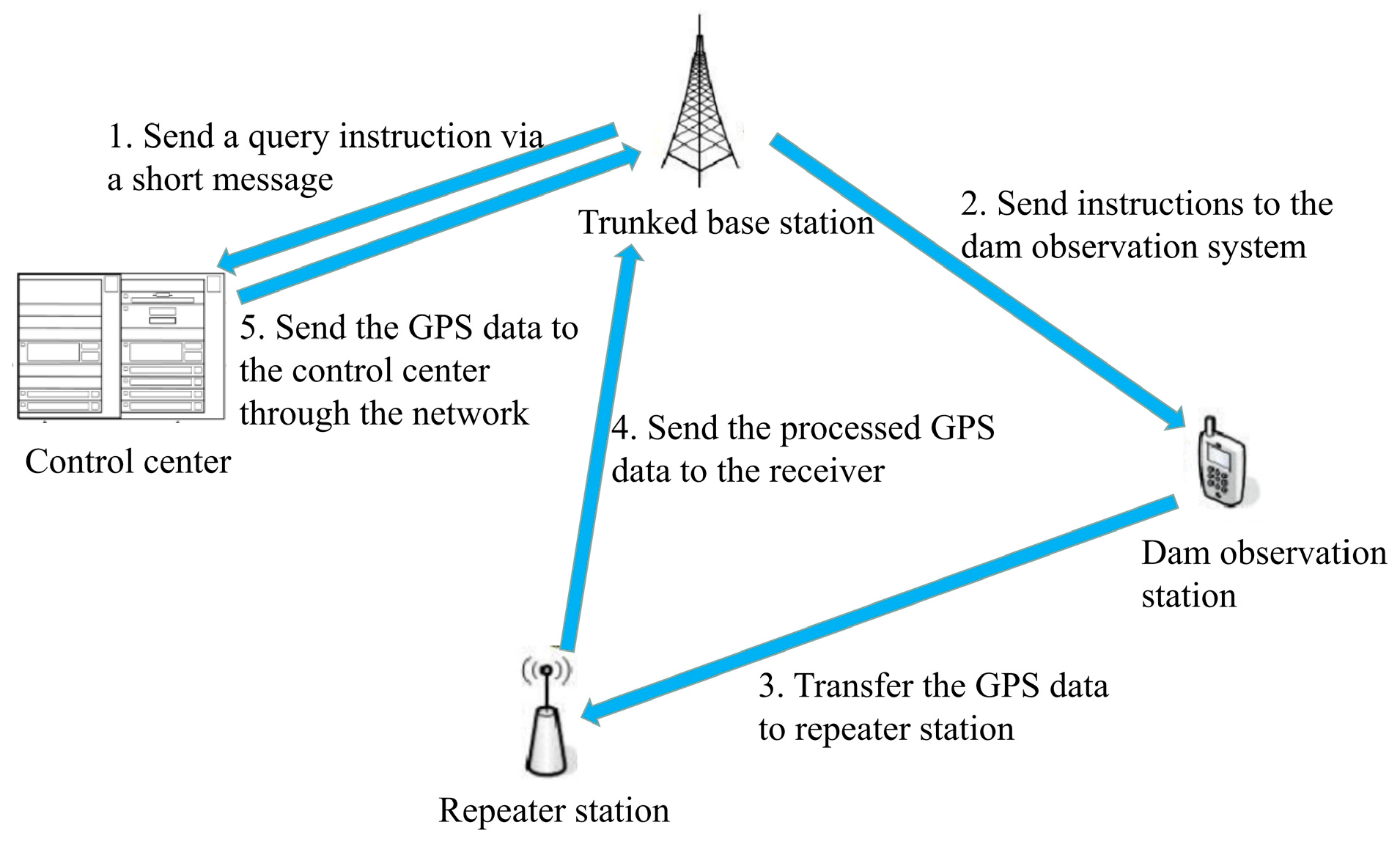
Figure 1. Schematic diagram of the GPS positioning.
Applsci 12 12103 g001
Figure 2. ELM neural network structure diagram.
Applsci 12 12103 g002
Figure 3. Flow chart of gross errors identification by LMS-IGG-ELM method.
Applsci 12 12103 g003
Figure 4. Actual and three-dimensional modeling drawing of the double-curved arch dam.
Applsci 12 12103 g004
Figure 5. Layout diagram of dam deformation monitoring.
Applsci 12 12103 g005
Figure 6. Scatter diagram of the displacement process with the gross errors in the measuring point PL13-3.
Applsci 12 12103 g006
Figure 7. Dam monitoring model after eliminating gross errors by the LMS-IGG-ELM method.
Applsci 12 12103 g007
Figure 8. Dam monitoring model after eliminating gross errors by the DBSCAN clustering algorithm.
Applsci 12 12103 g008
Figure 9. Dam monitoring model after eliminating gross errors by the Romanovsky criterion.
Applsci 12 12103 g009
Figure 10. Dam monitoring model after eliminating gross errors by the 3 σ method.
Applsci 12 12103 g010
Figure 11. Effect comparison chart of the dam validation segment after eliminating gross errors by the four methods.
Applsci 12 12103 g011
Table 1. Observation requirements of the three-level monitoring network.
Observation PointsSatellite Cut-Off Height Angle (°)The Number of Effectively Observed SatellitesObservation PeriodData Acquisition Interval (s)
Simultaneous
Observation
TotalQuantityObservation Time Duration (h)
The reference points≥15≥4≥92/30
Work basis points≥15≥4≥92≥530
Deformation observation points≥15≥4≥42≥530
Table 2. Treatment measure of IGG method weight.
Judgment ConditionMonitoring ValueMeasureWeight
| e | < k 1 σ normalreservation weight1
k 1 σ | e | < k 2 σ availablereduce the weightless than 1
| e | k 2 σ abnormaleliminate0
Table 3. Table of initial and final iteration weights of gross errors.
DataFirst Iteration Weights
( σ = 2.15)
Final Iteration Weights
( σ = 0.45)
DataFirst Iteration Weights
( σ = 2.15)
Final Iteration Weights
( σ = 0.45)
10 November 20160025 November 20160.92610
11 November 20160.841505 March 201700
13 November 2016006 March 20170.67720
14 November 2016007 March 201710
15 November 2016008 March 201710
16 November 2016001 August 201700
18 November 20160015 September 201700
19 November 20160016 September 201700
21 November 20160017 September 201700
22 November 20160018 September 201700
24 November 20160.6967019 September 201700
Table 4. Gross errors insertion positions and gross errors identification under the four methods.
DataRaw Data/mma*/mmb*/mmThe Identified Situation of Gross Errors
LMS-IGG-ELM MethodDBSCAN
Clustering
Algorithm
Romanovsky
Criterion
3σ Method
10 November 201638.85−5.8533.00
11 November 201638.754.2543.00
13 November 201638.82−5.8233.00
14 November 201638.819.1948.00
15 November 201638.78−6.7832.00
16 November 201638.707.3046.00
18 November 201638.67−6.6732.00
19 November 201638.608.4047.00
21 November 201638.52−6.0232.50
22 November 201638.48−6.4832.00
24 November 201638.474.5343.00
25 November 201638.483.5242.00
5 March 201726.056.9533.00
6 March 201725.72−12.2213.50
7 March 201725.363.6429.00
8 March 201725.003.5028.50
1 August 201728.2429.7658.00
15 September 201736.56−5.5631.00
16 September 201736.4826.5263.00
17 September 201736.7326.2763.00
18 September 201736.74−6.7430.00
19 September 201736.63−6.6330.00
a*: Gross errors of the displacement measurement value. b*: Displacement measurement after inserting gross error. √: Gross error is identified.
Table 5. Comparison table of gross errors identification rate of measuring point PL13-3.
Gross Errors Identification MethodNdrd(%)
LMS-IGG-ELM method22100
DBSCAN clustering algorithm1672.73
Romanovsky criterion313.64
3σ method29.1
Table 6. Comparison table of evaluation indicators.
Gross Errors Identification MethodFitting SegmentValidation Segment
MAERMSER2MAERMSER2
LMS-IGG-ELM method0.08900.12610.99980.32840.41010.9720
DBSCAN clustering algorithm0.37640.95260.97060.55720.61270.9375
3σ method0.41041.15820.98630.59470.73160.9106
Romanovsky criterion0.46841.53550.97620.86680.91070.8614
Publisher’s Note: MDPI stays neutral with regard to jurisdictional claims in published maps and institutional affiliations.