Abstract
The structural response of buildings to earthquake shaking is of critical importance for seismic design purposes. Research on the relationship between earthquake ground motion intensity, building response, and seismic risk is ongoing, but not yet fully conclusive. Often, probability demand models rely on one ground motion intensity measure (IM) to predict the engineering demand parameter (EDP). The engineering community has suggested several IMs to account for different ground motion characteristics, but there is no single optimal IM. For this study, we compile a comprehensive list of IMs and their characteristics to assist engineers in making an informed decision. We discuss the ground motion selection process used for dynamic analysis of structural systems. For illustration, we compute building responses of 2D frames with different natural period subjected to more than 3500 recorded earthquake ground motions. Using our analysis, we examine the effects of different structural characteristics and seismological parameters on EDP-IM relationships by applying multi-regression models and statistical inter-model comparisons. As such, our results support and augment previous studies and suggest further improvements on the relationship between EDP and IM in terms of efficiency and sufficiency. Finally, we provide guidance on future approaches to the selection of both optimal intensity measures and ground motions using newer techniques.
1. Introduction
Loss estimation in buildings due to earthquake shaking is critical for performance-based earthquake engineering (PBEE), which comprises four major components—seismic hazard, building response, probability of damage, and the costs due to losses and repairs. The engineering decisions on the retrofitting of structures are made based on probabilistic estimates of seismic performance of structures in terms of repair cost, casualties, and loss of functionality acceptable to stakeholders. In the first two stages of the PBEE framework, seismic hazard and building responses are estimated and represented in terms of “intensity measures” (IMs) and “engineering demand parameters” (EDPs). The implementation of a PBEE framework relies strongly on the ability of IMs to predict EDPs accurately. Each stage of PBEE is accompanied by uncertainties, both seismological and structural, influencing loss estimation [1].
Limited knowledge about earthquake source processes, Earth structure, and local site conditions contribute to uncertainties in seismological parameters, which in turn influence the estimation of IMs. Empirical ground motion prediction equations (GMPEs; also called ground motion models, GMMs) are available to predict IMs [2]. In GMMs, the complexities of the earthquake source process and seismic wave propagation in 3D heterogeneous Earth are simplified and then statistically accounted for when estimating ground motion intensities for future earthquakes. In addition to the seismological uncertainties, uncertainties in the structural response of buildings play a significant role in PBEE. These include the uncertainties in the estimation of stiffness, damping, and inertial characteristics of the building frame.
The characteristics of earthquake ground motion can be described by several types of IMs, related to the amplitude, frequency, and energy of ground motion. Therefore, to establish a meaningful relationship between ground motion and the corresponding structural response, it is necessary to investigate a broad range of IMs and analyze their correlations with building response over magnitude, distance, and site condition (e.g., Vs30).
IM-EDP relationships have been explored previously. Shome [3] coined the term “efficiency” to describe a given IM, whereby an efficient IM generates less variability (dispersion) about an estimated median in the predicted EDP. Efficiency is quantified by the standard deviation (“sigma”) in a prescribed EDP-IM relationship (Equation (1)). Padgett et al. [4] used “practicality” as another descriptor of an IM to examine direct correlations between IM and EDP. In practice, it is measured using the slope (regression parameter “b” in Equation (1) below) of the predictive relationship between IM and EDP. If the slope approaches b = 0, there is smaller dependence of the EDP on the IM, indicating that the IM is less practical to be used for structural design purposes.
Padgett et al. [4] also proposed “proficiency” as an indicator of IM, to investigate the combined effect of both efficiency and practicality. Proficiency is measured by a modified dispersion measure ( that quantifies the uncertainty introduced in a regression model as shown in Equation (1),
log (EDP) = a + b*log (IM) + δ
Here, a and b are coefficients obtained through linear regression; δ is the residual variability to characterize the variabilities between observed and predicted EDPs. For Equation (1), a lower dispersion measure indicates a more proficient IM.
Luco and Cornell [5] introduced the term “sufficiency” for IM-EDP relationships that are invariant over magnitude, fault mechanism, epicentral distance, and site class. More recently, Yeudy et al. [6] proposed a “steadfastness” measure to determine the robustness of IMs with respect to variations in building properties. It is computed as the ratio of mean of proficiencies when buildings are sorted with respect to the number of stories and total proficiency. Steadfastness becomes important in an urban setting where different building types exist.
Marafi et al. [7] defined “structurally independent”, “versatile” and “transparent” IMs that are invariant with respect to building types, also characterizing ground motion features such as peak values, duration and spectral properties. In addition to these proposed descriptors, “hazard computability” is important because existing seismic hazard maps are generally given in terms of PGA and period-dependent spectral acceleration (Sa(T)); however, ideally generating new hazard maps and fragility curves for a specific IM should be computationally and logistically simple [8,9].
Engineers have proposed a range of IMs to account for the differences in ground motion characteristics, but there is no consensus yet on which IMs, or combinations therefore, may be most appropriate. Thus, the first objective of this paper is to review the different IMs proposed in the literature, as well as the rationale behind their development. Due to the increased use of ground motion IMs in modern ground motion selection techniques, we examine the development of these techniques. The main objective of this paper, however, is to extensively evaluate existing IMs based on seismological and structural factors.
For this, we compile a list of ten IMs that are straightforward to calculate and for which GMMs are available. To model the structural response, we consider 18 2D reinforced concrete (RCC) frames with natural periods varying from 0.14 to 1.55 s; these we subject to over 3500 ground motion records. For various structural and seismological parameters, we then examine the correlations between frames and IMs. As a final step, we propose methodologies for utilizing these IMs in a manner that is both efficient and sufficient for calculating building responses. In the context of PBEE, the results of the paper are important in identifying the “ideal” combination of IMs depending on the situation.
2. Ground Motion Intensity Measures
With the increasing availability of strong ground motion data, new IMs are suggested to improve existing EDP prediction models. However, the efficiency of a particular IM depends on how well it correlates with the EDPs. An IM with stronger correlation with a particular EDP indicates that it is a good predictor. For example, spectral measures such as spectral acceleration (Sa(T)), spectral velocity (Sv(T)) and spectral displacement (Sd(T)) at the fundamental period of the structure are commonly found as efficient IMs based on correlation between EDP and IM [10,11,12]. However, these IMs do not account for higher vibration modes of the structure and non-linear effects, such as elongation of natural period [5,13,14,15,16,17]. To address this concern, several contemporary IMs have been proposed to accommodate the characteristics of both the ground motion and the structure [7,17,18,19,20,21,22,23,24,25,26,27,28,29,30,31,32,33,34].
2.1. Spectral Shape IMs
As discussed earlier, Sa(T) considers the response of a building with fundamental frequency T to a given ground motion record. However, due to the presence of higher modes, the response is also affected by ground motion contributions at other periods. Previous studies observed that the addition of spectral information in IMs reduces variability in the EDP-IM relationship significantly (Shome and Cornell [4], Carballo and Cornell [20], Baker and Cornell [21]). Shome and Cornell [4] reported an increase in efficiency for tall buildings by including spectral values at the second and third periods. Studies accommodate spectral shape by combining spectral values over a variety of periods [22,23,24,25,26].
Based on time history analyses of single degree of freedom structures (SDOF) with different hysteretic behaviors, Haselton and Baker [22] found the use of Sa at an elongated natural period to be more efficient. To account for period elongation, Cordova et al. [23] proposed a new IM (Equation (2)), with optimal values of and obtained by calibrating the response of four moment frame structures subjected to 16 near- and far-field ground motion records. Later, Mehanny [24] replaced the multiplier in Equation (2) with a relative lateral strength parameter . The efficiency was tested by subjecting 80 records to many SDOF systems with different hysteretic behaviors and values of . This provides flexibility to the IM to adapt for buildings with different non-linear behaviors.
Vamvatsikos and Cornell [17] showed that for structures with small contributions from higher modes, any reasonable choice for period elongation results in smaller dispersion. However, when higher modes are significant, two new IMs are proposed, listed in Equations (3) and (4), in which , , are empirically defined periods whose values were computed from time history analysis of 5, 9 and 20 story frames subjected to 30 ground motion records. It was observed that any reasonable value higher than the first three elastic periods for , and provides smaller dispersion [17]. Later, Lin [25] and Lin et al. [26] proposed modifications to Cordova [23] and Vamvatsikos and Cornell [17] by using three different frame configurations (4, 10 and 16 stories). The frames were subjected to 30 scaled and unscaled ground motion records. Equation (5) for short periods considers period elongation, and Equation (6) for long periods accounts for higher mode effects [25].
The above IMs only consider spectral information at certain periods and lack information of spectral shape. Bianchini et al. [27] proposed an alternative IM (Equation (7)) based on spectral values computed at 10 logarithmically spaced values between and . The efficiency of this IM when compared to Sa(Tf) and PGA was better for frames with higher mode effects. Tsantaki et al. [28] modified Equation (7) to incorporate P-delta effects (secondary effects when axial and transverse loads are applied simultaneously) by including a period band (Equation (8)). Similar IMs were put forward by Bojorquez and Iervolino [29,30], Eads et al. [31,32], and Xiao et al. [33,34].
For near-field ground motions, the spectral frequency content around the first mode of vibration is more efficient as IM than [19]. To account for it, Yahyaabadi and Tehranizadeh [35] proposed a root mean square-based IM, demonstrating that choosing optimal periods ensures efficiency regardless of the number of stories or ductility demand [35].
Some studies integrated spectral values over a range of periods to better account for spectral shape. Housner [36] proposed integration of a pseudo-spectrum velocity curve over the integration limits 0.1 and 2.5 s (Housner Intensity HI, Equation (9)). Von Thun et al. [37] proposed a similar IM using the same periods of vibration as Housner [36] but using the velocity response spectrum (velocity spectrum intensity VSI, Equation (10)). The measure has been suggested for assessing earthquake responses for earth and rockfill dams. Von Thun et al. [37] also introduced the acceleration spectral intensity (ASI), as they considered the information related to the acceleration spectrum more important for the seismic response and design of short-period dams (Equation (11)).
These IMs do not consider structural damage in the form of period elongation, and hence, several modifications were proposed to equations VSI and ASI by changing the integration limits. Kappos [38] replaced the integration limits in VSI by to , where and are period widths that are structure specific. Matsumura [39] replaced the integration limits with to , where is the yield period determined from pushover analysis. Martinez-Reuda [40] replaced the upper integration limit in Matsurma [39] with the hardening period of the structure. There is a need for this IM when strong ground motions from larger events or from site-amplified motions extend the natural period of building beyond the yield period.
2.2. Duration IMs
Shaking duration is another IM that strongly influences building response. The effect of ground motion duration has been studied for specific local site conditions (i.e., saturated soil deposits); however, the correlation of shaking duration and structural response needs to be further explored. Bommer and Martinez-Pereira [41] reviewed the role of different duration parameters in assessing structural damage. Subsequent studies observed cyclic fatigue effects under longer-duration earthquakes, leading to reduced strength and stiffness of masonry structures [42]. Based on Chandramohan et al. [43], significant duration (Tsig) is considered to be the most suitable IM for determining ground motion duration compared to other measures. Tsig is the time difference of 5% and 95% (or 75%) energy thresholds under the acceleration of time history. Marafi et al. [8] proposed to combine duration and spectral shape in a single measure (Equations (12) and (13)). IMdur in Equation (12) reflects the effect of duration, and IMshape incorporates the spectral shape information. The coefficients are based on regression analysis and account for sensitivities. In Equation (12), IMdur is given by Tsig, and IMshape is computed using Equation (13). in Equation (13) accounts for period elongation effects.
2.3. Energy IMs
The aforementioned IMs depend on structural configuration and are computed from spectral values. However, other IMs use accelerograms directly, which we a refer to as energy IMs. Energy represents the cumulative energy per unit weight absorbed by an infinite set of undamped single degree of freedom oscillators with a uniform distribution of periods on [44]. As energy measures of ground motion, root-mean-square acceleration (ARMS), Arias intensity (IA) and cumulative absolute velocity (CAV) are available. ARMS is calculated as the effective acceleration of ground motion during the significant duration (Equation (14)) and depends on both duration and energy characteristics of the record. In Equation (14), Tsig is the significant duration, and a(t) is the acceleration time series. Arias intensity (IA), (Equation (15)) represents the energy dissipated during the entire record duration. Cumulative absolute velocity (CAV, Equation (16)) is calculated as the area under the absolute accelerogram, thus representing the continuous accumulation of acceleration in a ground motion record. CAV is a useful measure of the onset of structural damage.
The IMs summarized above incorporate duration and amplitude characteristics. However, some studies refer to IMs accounting for amplitude, duration and frequency content also as energy-based IMs. To equate the motion for a damped SDOF system subjected to ground acceleration, each term is multiplied by differential increments of displacement and are integrated in the time interval (0, t) to obtain Equation (17) [45]. Equation (17) represents kinetic energy , damping energy and absorbent energy on the left side, while the right side represents relative input energy . Housner [46] defined actual damage to structures as the difference between relative input energy and damping energy. Equations (18) and (19) are equivalent velocities that represent the relative input energy and damage energy, respectively.
2.4. Vector Valued IMs
To account for lack of information in scalar IMs discussed above, some authors propose vector-valued IMs. Elefante et al. [47] proposed a combination of PGA and moment magnitude Mw as a more efficient predictor than PGA alone. A combination of Sa(Tf) and ) (Equation (20)) was proposed by Baker and Cornell [48]. For a particular magnitude Mw, distance R and other site-source properties denoted by , , a spectral shape measure is defined as the number of standard deviations that separate a given lnSa(Tf) value from the mean predicted from a ground motion model (Equation (20)). Baker and Cornell [1] also proposed a combination of Sa(Tf) and R = Sa(T*)/Sa(Tf). Here, T* is any other period that is chosen to represent the spectrum’s shape, and T* = 2Tf and T* = T2 for accounting for period elongation or higher mode effects was suggested by Baker and Cornell (2008a) [1]. Other vector-valued measures that use Sa(Tf) and a few unitless quantities are discussed in the literature. Bojórquez et al. [49] proposed IA, normalized by the product of PGA and PGV, whereas Theophilou et al. [50] proposed SdN(Tf,T2), determined by integrating the displacement response spectrum and normalizing with Sd(Tf).
The above summary of proposed IMs illustrates that with the ever-increasing number of IMs available in the literature, it is important to understand their correlation with building response. The number of buildings instrumented to record the shaking response during earthquakes is small. However, due to the efforts of the California Strong Motion Instrumentation Program (CSIMP) and the Japanese Building Research Institute (BRI), this database is also growing. Perrault and Guéguen [51] used these data to calibrate existing EDP prediction models; they found that the variability in total drift ratio can be reduced by classifying the buildings based on construction material and height. Astorga et al. [52] developed a flat file of some of the EDPs and IMs calculated from the recorded building responses and earthquake ground motions from CSIMP and BRI databases.
Recent research has focused on ensuring that hazard consistency is enforced during the selection of records, rather than covering response estimates for ground motions generated by all possible scenarios. Therefore, modern ground motion selection techniques account for a variety of IMs in the process of record selection. Let us therefore review different methods of selecting ground motions in the following section.
3. Ground Motion Selection Techniques
Non-linear phenomena, such as plastic hinge deformation and soil-structure interactions, contribute to intricate building responses. To capture these complexities, non-linear dynamic analysis of buildings is necessary. A linear elastic dynamic analysis, however, is useful for multiple-supported infrastructures, such as bridges, because of dominant vibration modes [53]. Linear analysis uses a response spectrum as input, while non-linear analysis requires a complete earthquake ground motion time history as input. As computing capabilities have advanced, seismic building codes recommend using non-linear dynamic analysis. However, near-field ground motions themselves are very complicated due to intricacies of the earthquake rupture process, seismic wave propagation in 3D heterogeneous Earth, and local site effects [54]. Ground motion selection is thus key to determining whether a dynamic analysis provides a building response that is “relevant” for the site. Because of the subtleties involved in the selection process, this section provides an overview on available selection techniques.
Results of seismic hazard analysis (SHA), either deterministic (DSHA) or probabilistic (PSHA), are required to aid in the selection process. Using a deterministic approach, the magnitude of the maximum credible earthquake (MCE) for the site of interest is identified based on the tectonic setting and past data [55,56]. As a result, records are selected based on the magnitude–distance combinations that are likely to generate the highest ground motion amplitude. A probabilistic approach involves integrating the expected seismicity over a period and a chosen magnitude range (i.e., all earthquakes larger than moment magnitude Mw 4) to estimate strong motion parameters (such as peak ground acceleration, PGA, or spectral values Sa(T)), including their uncertainties [57,58,59,60,61]. Subsequently, hazard curves are computed for specific strong ground motion parameters. A uniform hazard spectrum (UHS) can then be derived and used for the time history selection process. In the next few sections, we review different ground motion selection approaches described in the literature.
3.1. Selection Based on Seismological and Site Characteristics
Several methods were initially proposed to select ground motions based on magnitude and epicentral distance. Young et al. [62] developed a database of records with sets based on magnitudes and site distances. As expected, earthquake magnitude is an important factor for earthquake selection in other studies (Bommer and Acevedo [63], Stewart et al. [64]). It is common for the search window range of magnitude and distance to be adjusted in order to include more records. Magnitude ranges of 0.2 Mw and 0.25 Mw are proposed by Bommer and Acevedo [63] and Stewart et al. [64].
Iervolino and Cornell [65] demonstrated that selection based on magnitude and distance is not justified. For this purpose, Iervolino and Cornell [65] analyzed two classes of records for a target site (Mw = 7.0 and R = 20 km). One class of records is chosen based on magnitude and epicentral distance, while another class of records is chosen arbitrarily from an earthquake catalogue, but scaled. Generally, scaling is performed so that spectral values at natural periods of structures are closer to UHS at those periods. These records were subjected to different SDOF and MDOF structural systems with different natural periods and configurations, hysteresis relationship and material of construction (reinforced concrete and steel). In terms of building response from these two sets, no significant difference was detected to justify a careful selection of records. In addition, Bazzurro and Cornell [66,67] demonstrated that displacements of nonlinear structural elements are independent of epicentral distance. Nevertheless, magnitude and distance are still used in practice for initial selection of records, at least when they are readily available.
In record selection, the soil profile is also considered if available. Depending on the velocity layers of the soil beneath the building, ground motion may be amplified or de-amplified. Vs30, time-averaged shear wave velocity in the top 30 m, is usually used to represent the soil characteristics. Based on Vs30, seismic codes characterize the type of soil in different categories such as rock, stiff soil, and loose soil (NEHRP). Bommer and Scott [68] discovered that when soil type is used to select records from a strong motion database comprising 1600 records from 1933 to 1995, the number of records available for selection is dramatically reduced.
In addition to the factors discussed above, strong motion duration is critical for building performance and has to be included when choosing ground motions. However, strong motion duration depends on the rupture duration (the time it takes from the onset of the rupture process until it is completed) on the causative fault, and thus, it is already partially considered in magnitude (larger-magnitude earthquakes have longer rupture duration). We remark that the effect of strong motion duration also depends on the demand indexes that are considered. For example, duration has no effect on peak deformation parameters but affects hysteretic energy and the number of cycles. ASCE Standard 4–98 [69] proposes to take a record’s duration as an indication of the ground motion at a site at a given seismic hazard level.
Furthermore, the seismotectonic settings need to be accounted for, as they also affect strong ground motion. Kawaga et al. [70] demonstrated that ground motions at the surface of buried faults are stronger than those at the surface of surface ruptures at 1 s periods. Furthermore, shallow-crust earthquakes show different peak and spectral amplitudes versus subduction zones (Lin and Lee, [71]). Therefore, these parameters should be considered when selecting a ground motion. As a result of these constraints, the pool of records is significantly reduced during the selection process. In several studies, however, similar ground motions and underlying source mechanisms have been found for earthquakes in different regions (Boore et al. [72], Stafford et al. [73]).
3.2. Selection Based on Spectral Values
In a building code framework, spectral matching, which involves matching the response spectrum of candidate records with the target spectrum, is recommended. This target spectrum is characterized by a smooth design spectrum at different periods. It is possible to verify candidate response spectra with target records using different approaches (Ambraseys et al. [74], Iervolino et al. [75]). Ambraseys et al. [74] proposed Equation (21) to verify the spectral compatibility of records. Drms considers the difference of spectral values between a candidate and target spectrum. The thresholds for Drms depend on the period range of interest and number of records required. Alternative approaches involve the scaling of spectral values at longer periods (Beyer and Bommer [76]).
A building code’s design spectrum is an approximate version of the Uniform Hazard Spectrum (UHS), which is more common in practice. The UHS is calculated in the PSHA framework using spectral accelerations at different periods for the same hazard levels. Baker and Cornell [48], however, argue that UHS is ineffective for selecting ground motions, and instead propose a conditional mean spectrum (CMS). Baker and Cornell [48] state that the UHS does not represent the spectrum of any individual ground motion; hence, it is unlikely that an individual ground motion will exceed the hazard level at all periods. Therefore, building designs based on UHS are more conservative.
To propose CMS, Baker and Cornell [48] used deaggregation analysis of PHSA. This information pertains to earthquake events (Mw, R and ) that are most likely to produce a specific target spectral value over a particular period. The value defines how much larger a target spectral value at a given period is compared to the predictions of a GMM (GMM of Abrahamson and Silva [77] is used in the original study [48]). A fundamental principle of CMS is that the spectral value obtained from deaggregation of a given period does not necessarily apply to other periods. A constant value of would represent a standard UHS curve.
From a large suite of ground motions, Baker [78] observed a high correlation between and , compared to and . We can use this correlation relationship to determine the trend over different periods, provided we know what the information was during a particular period. The target spectrum can be derived from mean values of , which are computed as a multiplication of at a known period and correlation coefficients between at known and unknown periods derived from a ground motion database. The procedure to compute CMS has been illustrated in Baker [79]. Equations to compute mean and median CMS values are given in Equations (22) and (23).
Baker and Jayaram [80] computed based on statistical analysis of joint distributions of spectral accelerations. Ground motions are selected by matching the mean target response spectrum (Equation (23)), which is computationally inexpensive. The variance of target response spectrum can also be calculated and holds crucial information. Ground motion selection is then based on optimization schemes as those proposed by Jayaram et al. [80] and Baker and Cynthia [81]. In these algorithms, simulated realizations and target spectra are generated randomly, and records are then selected based on the difference between the means and variances of the simulated realizations and the target spectra. CMS can also be referred to as conditional spectra (CS) when both the mean and variance of the target spectra are matched. Recent studies by Kwong et al. [82] have extended the CS approach to include both vertical and horizontal records and to select records based on multiple components.
There is a major limitation when using CS, due to the fact that the response spectrum does not accurately represent the seismic response of structures. Several IMs were proposed that are associated with both structural and seismological parameters, as discussed in Section 2. This led Bradley [83,84] to develop the generalized conditional intensity measure (GCIM), a more holistic approach to include any IM in conditional distribution calculations. The selection can be based on a scalar or a vector of intensity measures. To be consistent with current practices in seismic hazard analysis, Lin et al. [85] further modified the CS algorithm by allowing different GMMs to be used to calculate . Highlighting the importance of the spectral correlation structure with periods, Ha and Han [86] developed a methodology considering correlation structure in the selection process along with target spectra. This is very important when selecting simulated ground motions that do not necessarily follow the same correlation structure as recorded ground motions [87]. Kohrangi et al. [88] developed a compound target spectrum that incorporates multiple target spectra at multiple IM levels into a single spectrum. Kohrangi et al. [89] presented a newer CMS to use average spectral acceleration over a period range (AVGSa) instead of Sa(Tf) as the conditioning IM.
3.3. Selection Based on Causal Parameters and Spectral Shape
Ground motion databases around the world are increasing rapidly, with NGA West2 being six times larger than NGA West1. Hence, Tarbali and Bradley [90] have argued for screening candidate ground motions according to Mw, R and Vs30 (causal parameters) prior to applying the selection based on spectral shape. The reason is that applying traditional CS and GCIM techniques to a very large database will result in the selection of records that the structure may never encounter. To perform this screening, Mw, R and Vs30 can be bound using deaggregation results from PSHA. If the bounds are too narrow, there would be few records left for selection, and if they are too wide, then incompatible records would be left. As a result, it is necessary to carefully select the bounding values. The following bounding limits for Mw and R (Table 1) were proposed by Tarbali and Bradley [90], where Mw 1% represents the first percentiles of marginal deaggregation distribution results of Mw.

Table 1.
Bounding limits proposed by Tarbali and Bradley (2016) [90].
A different method of analyzing this problem is proposed by Spillatura et al. [91]; they advocate that records should be screened after the spectral shape selection has been completed. In their approach (referred to as CS-MR), records selected based on their spectral shape are discarded based on the desired Mw and R bins. Records that do not fit into desired Mw–R bins or those that exceed each bin’s contribution to a particular hazard level are removed. This is followed by the addition of desired ground motions from underrepresented Mw–R bins, resulting in a set of results that are consistent with both the target spectrum and the deaggregation results.
The previous sections illustrate that ground motion record selection has become an increasingly complicated process that includes consideration for a variety of seismological properties. Therefore, it is necessary to investigate the relationship between IM-EDP in relation to various seismological parameters. Let us therefore discuss in detail how different parameters (structural and seismological) affect the relationship between IM and EDP. We also provide recommendations for future improvements.
4. Recommendation on Improving the Efficiency of Intensity Measures
In this section, we analyze efficiency and sufficiency of IMs by computing statistical correlations between EDPs (maximum inter-story drift ratio) and ground motion IMs from a set of near-field records in the NGA West2 database. We consider 2D reinforced concrete (RC) frame buildings with different natural periods and perform non-linear time history analysis to obtain inter-story drift ratios.
For each IM value, we investigate correlations of EDPs over magnitude, epicentral distance, and site class for different natural periods of structures. We then examine correlations using multi-parameter linear regression models to assess the change in efficiency and sufficiency characteristics. Our results confirm and augment previous findings, while we also provide recommendations on how the efficiency and sufficiency of IMs can be improved. We discuss the ground motion database, intensity measures, and building models in the following sub-section.
4.1. Ground Motion Database, Intensity Measures and Building Response
We select over 3500 near-field ground motion records from the NGA-West2 database with epicentral distances Repi ≤ 100 km for moderate-to-large earthquakes in the magnitude range Mw 5.0–8.0 (Figure 1). Figure 1 (right) displays the histogram of ground motion records, sorted into magnitude bins 5–6, 6–7 and 7–8. There are a total of 3582 records from 105 events of which 41% are reverse faulting, 22% of strike-slip and the remaining events are normal and oblique mechanisms. Site conditions for these ground motion recordings are site class A–E, based on Vs30 [92]. The two horizontal components of ground motion are used individually to compute the structural response for different building frame configurations.
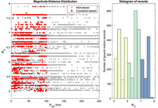
Figure 1.
(Left) Magnitude Mw versus epicentral distance Repi for strong-motion recordings in the NGA west 2 database (gray dots). Red points show the dataset used in this study, focusing on the near-fault region with maximum epicentral distance Repi = 100 km, leading to 3582 records from 105 events. We consider only magnitudes Mw > 5 to ensure a significant response of the structure; 41% of records are from reverse-slip, 22% each from strike-slip and oblique-slip and remaining from normal slip events. (Right) Histogram of records sorted with respect to magnitude. The highest strong motion records fall in 6.0 to 7.0 magnitude category, followed by 7.0 to 8.0 range.
For the chosen records, we compute ten widely used IMs, categorized as (i) peak ground motion parameters (PGA, PGV and PGD), (ii) spectral and duration parameters (Sa(T), ASI, VSI), and (iii) energy parameters (ARMS, CAV, IA) to accommodate the amplitude, spectral, duration and energy.
Figure 2 summarizes the distance dependence of these IMs for the selected ground motion dataset. The solid black line represents the moving window average of IMs. We observe a more rapid distance decay of PGA than for PGV; however, PGD remains almost invariant over distance. For spectral measures, a rapid decay with distance for ASI is observed compared to VSI. For the three energy measures, we find that ARMS and IA decrease with distance, while CAV remains almost constant. Tsig increases with distance, as many recording sites are located in sedimentary basins where the intensity of ground shaking and its duration increase with distance due to the slow arriving surface waves.
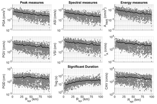
Figure 2.
Variation of peak amplitude, spectral, temporal, and energy intensity measures with epicentral distance. Black solid lines represent the moving average. PGA and PGV decrease with epicentral distance, whereby the attenuation of PGA is stronger. PGD follows a constant trend with distance. Spectral intensity measures and energy measures decrease with distance, except for CAV, which remains almost invariant. Significant duration (Tsig) increases with distance.
To analyze correlations between IMs and building response, we model two-dimensional (2D) reinforced concrete (RC) frames, considering 18 different symmetric and asymmetric configurations with natural periods varying from 0.14 to 1.55 s. Rayleigh damping is used to model viscous damping in the structures and frequencies corresponding to the first mode and mode98 (mode at which mass participation exceeds 98%), which are used to evaluate damping coefficients. Table 2 summarizes our chosen building configurations that represent typical RC frames designed according to building code recommendations. Figure 3 and Table 3 describe the geometry and member configurations of three frames. (#3, #9 and #14 in Table 2).
Table 2.
Structural properties of selected frames.
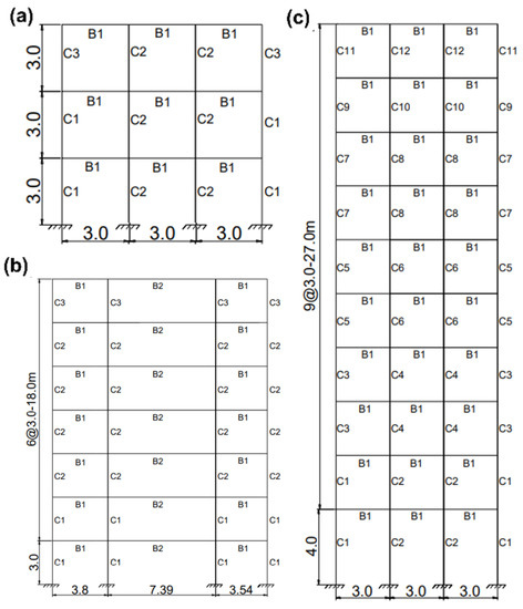
Figure 3.
Geometric description of Frames #3, #9 and #14 in Table 2. All dimensions are in meters. (a–c) corresponds to short, intermediate and long period structures.
Table 3.
Sectional properties of Frames #3, #9 and #14 in Table 2.
The material models of concrete and steel employed in this study are concrete02 model [93] with linear tension softening and reinforcing steel with strain hardening ratio of 0.005. A description of the material models adopted for concrete and steel as well as values for each parameter are shown in Figure 4 and Table 4. The corresponding equations of motion are solved based on the finite-element method implemented in OpenSees [94]. All 2D-RC frames are assumed to be fixed at the column base. We apply the same dead load (DL)/live load (LL) combination to all the frames as (100%DL + 25%LL) to ensure equal contribution of inertial effects in the modal analysis of the frames.
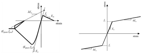
Figure 4.
Material models for concrete (left) and steel (right) adapted from Opensees manual [94]. In the concrete model, fpc stands for concrete compressive strength at 28 days and fpcu for concrete crushing strength. Eo and Ets stand for initial elastic tangent and tension softening stiffness, respectively. Ɛpsco and Ɛpscu are concrete strain at maximum and ultimate strengths, respectively. represents the ratio between unloading slope at ultimate strain and initial slope. ft is the tensile strength of concrete. In the steel model, fy stands for yield stress in tension, Eo is modulus of elasticity and b is the strain hardening ratio. The values adopted for concrete and steel models are given in Table 4.
Table 4.
Material properties for concrete and steel models used for modeling frames.
To simulate the response of a frame subjected to earthquake ground motion, we perform a nonlinear direct-integration time history analysis using the Newmark Scheme [95] to estimate the energy demand parameter (EDP). For the EDP, we use “maximum inter-story drift ratio” (ISD), which is more suitable for multi-degree-of-freedom structures [96]. Damage states and the corresponding drift ratio thresholds are defined depending on the seismic design level, performance level, and building typology (height, material or construction type) [97]. The correlations between IM and EDP are discussed in the next section.
4.2. EDP-IM Relationship
To examine correlations between the various parameters of interest, we first extract the inter-story drift ratio (ISD) computed for all considered frames. Using the Pearson correlation coefficient, we then quantify the correlation between ISD and IMs by applying linear regression to fit the measured ISDs with a given IM (Equation (1)).
Figure 5 shows the variation of ISD for six of ten different IMs, including the correlations coefficient (), efficiency (), practicality () and proficiency measures. The mean predictions for the EDP along with the standard deviations (solid and dashed lines) are plotted for each IM. Both peak measures, PGA and PGV, show similar correlation () with EDP; however, the variability is lower for PGV. and IA are good indicators for spectral and energy measures of IMs, respectively. Among all IMs, the correlation of Tsig with inter-story drift is smallest. ASI, PGV and VSI show similar proficiency; however, proficiency is higher for IA and Tsig.
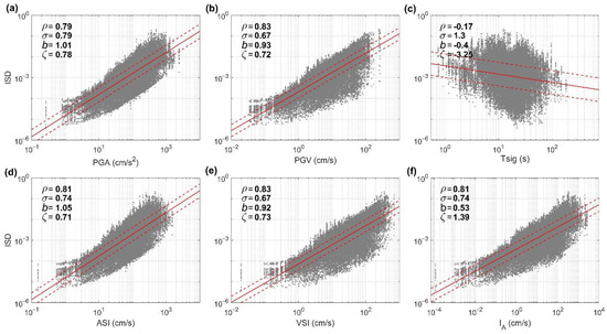
Figure 5.
Correlation between inter-story drift ratio and six intensity measures. Bold numbers denote the correlation coefficient, efficiency, practicality, and proficiency of IMs with respect to equation (red line). Variability (sigma) is computed as the mean of residual () from equation (a,b) correspond to peak measures (PGA, PGV) and (d,e) correspond to spectral measures (ASI, VSI). (c,f) are for significant duration (Tsig) and Arias intensity (IA).
For comparison, Table 5 shows the correlation properties of 15 different IMs, including the IMs proposed by Cordova et al. [23], Vamvatiskos and Cornell [17], Lin et al. [25], Bianchini et al. [27] and Tsantaki et al. [28]. Larger correlations for spectral measures compared to other IMs are consistent with the results of Astorga et al. [52], who used building response of existing structures exposed to earthquake motions. The current overall correlation properties do not distinguish buildings with different natural periods; hence, we divide frames by their natural periods and examine the effect on the correlations.
Table 5.
Correlation, efficiency, practicality, and proficiency of 15 IMs. IMCordova, IMVamvatsikos, IMLin, IMBianchini and IMTsantaki are computed using Equations (2)–(5), (7) and (8), respectively. VSI, ASI, ARMS, IA and CAV are computed using Equations (10) and (11) and Equations (14)–(16).
4.2.1. Period Dependence
In this section, we investigate the structural period dependence of the estimated correlations by classifying frames by their natural period. Figure 6 illustrates the variation of correlations of peak measures, spectral measures, and energy measures with fundamental period of the structure. We observe that correlations of peak measures show significant variations with fundamental period (Figure 6a). PGA exhibits strong correlations for short-period structures (T < 0.4 s), and PGV shows strong correlations for intermediate-period (0.4 < T < 0.8 s) and long-period structures (0.8 < T < 1.2 s). Although the correlations with PGD reveal an increasing trend with period, PGD does not saturate to a constant value for the structural periods considered. Therefore, we conclude that PGD is not a good IM indicator for building frames for this range of natural periods.

Figure 6.
Correlations between IMs and EDPs as a function of structural period. (a–c) are for peak, spectral and energy measures, respectively. PGA and PGV exhibit good correlation; PGA decreases with period. The correlation with PGV increases with period, with a slight decrease beyond 1.2 s; the correlation with PGD is moderate and increases with period. Among the spectral measures, the correlation for ASI is similar to that of PGA, and VSI is similar to that of PGV. For long period structures, correlation with VSI remains almost constant. Sa(T) shows strong correlation for short-period frames and remains constant for longer periods. Among the energy measures, ARMS and IA decrease with periods, while CAV remains approximately constant.
Figure 6b depicts the variation of correlations between spectral parameters and ISD with the fundamental period of structures, as well as the correlations between significant durations and Sa(T). Sa(T) seems to be an applicable IM over the entire range of natural period. Since ASI and VSI are influenced by high-frequency and intermediate-frequency contributions of the pseudo-spectral acceleration and velocity response, they exhibit strong correlations at the corresponding natural periods. The good performance of spectral measures over peak measures to predict building response is consistent with previous studies [10,11,12,98]. This can be attributed to the fact that spectral shape of ground motion affects the building response and that peak measures are not representative of the shape of the spectra. Figure 6c shows the period-dependent correlations of energy measures. ARMS and IA exhibit correlations of around 0.9 for short period structures and decrease with period. For CAV, correlations are around 0.8 and remain almost invariant with the natural period.
For the building frames modeled in our study, we do not observe any correlation of ISD with ground motion duration, Tsig. Several studies have shown that longer ground motion durations impart a larger number of cycles of earthquake loading on the structure, thus causing significant impact on structural response [99,100]. However, the selected frames do not account for effects of structural fatigue; therefore, the responses do not correlate with duration.
Despite high correlations and low variability, peak and spectral measures (except Sa(T)) are not entirely structurally independent. Therefore, it is important that the selection of these IMs must be made based on the fundamental vibration mode of the structure. Our analysis shows that for very small periods (<0.3 s), PGA is a good indicator, while for periods (0.3–0.6 s), ASI is an efficient indicator. For moderate (0.6–1.2 s) and long periods (>1.2 s), PGV and VSI better capture the response of structure, respectively. In the next section, we examine the effect of magnitude Mw and epicentral distance Repi on the correlations between IM and EDP.
4.2.2. Magnitude and Epicentral Distance
To further discuss the sufficiency of the selected IMs, we examine the dependence of correlations with event magnitude and epicentral distance, considering three different magnitude bins: 5.0 Mw 6.0 (I), 6.0 < Mw 7.0 (II) and 7.0 < Mw 8.0 (III). We compute correlations between ISD and IMs using a moving window approach for each magnitude bin. From all 2D-RC frames, we select three frames with fundamental periods to represent a short (Tf = 0.35 s), intermediate (Tf = 0.82 s) and a long period (Tf = 1.21 s) structure (frames #3, #9, and #14 of Table 1) (henceforth denoted as SP, IP, and LP structures). The distance-dependent correlations of peak, spectral, and energy measures for the different magnitude classes are summarized in Figure 7, Figure 8 and Figure 9.
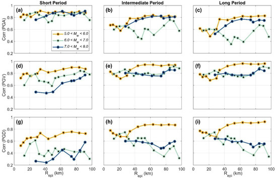
Figure 7.
Distance-dependent correlations of peak measures (PGA, PGV, PGD) for different magnitude bins (Mw 5–6, Mw 6–7 and Mw 7–8) (panels a–i). Rows correspond to variations in correlations of PGA, PGV and PGD for three different types of structures—short period, intermediate period and long period (SP, IP and LP). Correlations of PGA and PGV are almost invariant for SP and IP/LP structures, respectively (panels a,e,f). For IP/LP structures, correlations of PGV increase with distance for magnitude bins Mw 6–7 and Mw 7–8. PGD shows significant distance and magnitude dependence for all types of structures.
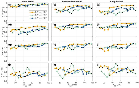
Figure 8.
Distance-dependent correlations of spectral measures (ASI, VSI, Sa(T)) for different magnitude classes (Mw 5–6, Mw 6–7 and Mw 7–8) (a–l). Rows correspond to variations in correlations of ASI, VSI and Sa(T) for three different types of structures (SP, IP, LP). Correlations of ASI (a–c) and VSI (d–f) are almost invariant for SP and IP/LP structures, respectively, and do not show any noticeable magnitude dependence. Correlations of Sa(T) vary less for SP structures than IP or LP.
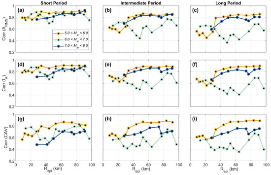
Figure 9.
Distance-dependent correlations of energy measures (ARMS, IA, CAV) for different magnitude classes (Mw 5–6, Mw 6–7 and Mw 7–8) (a–i). Rows correspond to variations in correlations of ARMS, IA and CAV for three different types of structures (SP, IP, LP). Energy measures, especially ARMS (a–c) and IA (d–f), show very similar variation in correlations as that of PGA in Figure 7.
From the ten IMs, we find that correlations of PGA and ASI are invariant with magnitude and distance for SP structures (Figure 7a and Figure 8a). For IP and LP structures, correlations of PGA and ASI decrease for magnitude bin Mw 6–7 in the distance range of 40–70 km. Similar findings appear for energy measures (ARMS, IA and CAV). This may be a consequence of several seismological effects such as directivity effects and/or site effects. Correlations with peak measures are strongest for small magnitude events and then decrease with magnitude, especially in the case of PGV and PGD. The dependence on event magnitude is not significant for Sa(T) at different distance bins (Figure 8). Among all energy measures, ARMS and IA show the lowest correlation with respect to magnitude and distance (Figure 9).
For the epicentral distance range 30–80 km, distance-dependent correlations are larger for small magnitude events, while correlations with IMs are similar across all magnitude classes beyond 80 km. This behavior of the IMs is expected, because the building response is non-linear close to the source and tends to a more elastic at larger distances from the source. Figure 10 shows the logarithmic ratio of observed response (EDP) and elastic limit for SP, IP and LP structures for different magnitude classes. The elastic limit is taken as the total elastic drift ratio and is computed from pushover analysis. As distance increases, the response becomes linear (ordinate less than zero). Since at far distances, the response is linear for most of the records, the correlations are similar for all magnitude classes. For intermediate distances, the response is significantly linear only for magnitude bin I (5 < Mw < 6), with stronger higher correlation than the other two classes.
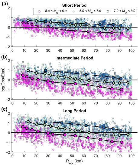
Figure 10.
Logarithmic ratio of observed EDP and elastic limit for SP, IP and LP structures (a–c). The black solid line is the elastic limit for SP, IP and LP structures respectively. The colors show ground motion grouped into different magnitude bins. The solid lines are the moving averages of logarithmic ratio of observed EDP and elastic limit. As epicentral distance increases, the records rather produce elastic responses and hence show larger correlations.
Let us now analyze the relationship between IM and EDP based on another seismological parameter, the site class.
4.2.3. Site Class
We now discuss the influence of soil types on the correlations, by grouping the ground motions according to site classes B, C, D and E, using the NEHRP soil classification. Site class A is not considered due to the small number of available records (only 0.2% in our database). To present these correlations, we again use the selected SP, IP, and LP frames (Figure 3). Figure 11 reveals that site class does not affect the correlations of PGA and ASI for SP structures and PGV and VSI for IP/LP structures. High correlation of PGV and VSI irrespective of site class was also reported by Ozmen and Inel [101]. For PGD, the correlations decrease with site class. However, the correlations with PGV decrease with site class (B to E) or shear wave velocity Vs30. ASI and VSI exhibit correlations similar to PGA and PGV. Among the spectral measures, the correlation with Sa(T) shows the least variation with site class. Among the energy measures, ARMS and IA show good correlations and smallest dependence on site class (Figure 11). However, the correlations with CAV decrease with site Vs30.
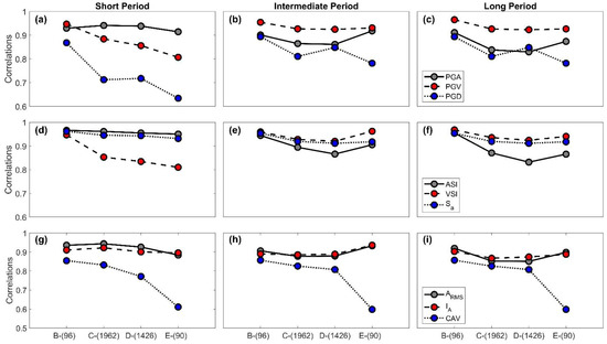
Figure 11.
Dependence of correlations of intensity measures with site classes B, C, D and E (based on NEHRP recommendation), along with number of records per site class (in brackets). Rows represent variations in correlations of peak measures, spectral measures and energy measures for three different types of structures (SP, IP, LP). For short-period structures, the correlations of PGA appear to be independent of site class (a). For IP/LP structures, correlations of PGV are invariant with site class (b,c). PGD correlations decrease with site class (c). For spectral measures, ASI and VSI exhibit correlations similar to PGA and PGV (d–f). For energy measures, ARMS and IA show good correlations and least dependence with site class (g–i).
In summary, for a given natural period of interest, ASI and VSI represent sufficient IMs for SP and LP structures, respectively. Figure 12 displays the variation of ISD with Vs30, documenting that the mean response does not change much with soft sediment shear velocity. However, our assumptions related to the building models simplify the interaction with the sedimentary layers by using a fixed support at the column bases. Furthermore, lateral deformation of structures in loose soils will be affected by rocking and rotations of foundations, which are not considered in our approach.
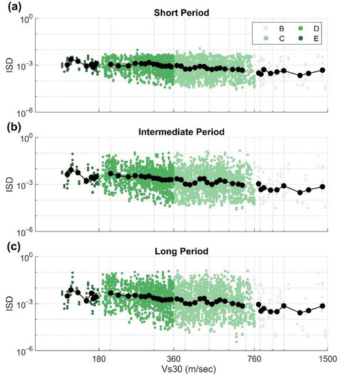
Figure 12.
Variation of inter-story drift (ISD) ratio with Vs30 for SP, IP and LP structures (a–c). Black line indicates a moving window average of ISD. The mean ISD (black line) does not change significantly for different ranges of Vs30.
4.3. Analysis of Functional Forms
Thus far, we have used the standard functional model (single parameter regression model) to define relationships between IMs and EDP (Equation (1)). However, this model does not sufficiently capture the complex interaction of the two. We observe that by including the seismological parameters in the functional form, the efficiency in predicting EDPs increase on average by 10% for the selected IMs. Perrault et al. [51] considered a multiple IM approach by including PGA, CAV, Sa(T) and Sv(T) within a frequency range close to the fundamental period of the structure. Yeudy et al. [6] included seismological parameters (Mw and Repi) directly in the functional forms (Equation (24)), noticing an increased efficiency and sufficiency with respect to Mw and Repi.
log (EDP) = a + b*log (IM)+ c*log (Mw)+ d*log (Repi) + δ
By extending Equation (24), we show that IMs can be made even more efficient and sufficient by including soil stiffness parameter (Vs30) and structural period (Tf) in the functional forms (Equations (25) and (26)).
However, different combinations of these parameters may generate a series of models with the risk of either over- or under-fitting. We therefore apply the Akaike information criteria (AIC) to determine the statistical quality of all possible models arising from these parameters. Table 6 lists AIC scores for different input parameters while using PGA and PGV as IMs. As expected, AIC scores are lowest when all parameters are considered in the regression model (bold values in Table 6). Similar results are found considering other IMs.
log (EDP) = a + b*log (IM) + c*log (Mw) + d*log (Repi) + e*log (Vs30) + δ
log (EDP) = a + b*log (IM) + c*log (Mw) + d*log (Repi) + e*log (Vs30) + f*log (Tf) + δ
Table 6.
Analysis of Akaike information criterion.
Table 7 summarizes efficiencies and proficiencies for various IMs and the different functional forms defined in Equations (24 and 26). We find that the suggested modifications to Equation (1) increase the efficiency and proficiency. We also find that the fundamental period of the structure plays an important role in predicting EDP, hence including the structure’s period (Equation (26)), and soil stiffness parameter (Vs30) improves the predictions remarkably (bold values in Table 7). We observe significant increases of 45% and 19% for Sa(T) and ASI, respectively, with respect to the standard implementation.
Table 7.
Efficiency and proficiency characteristics of various functional forms and IMs.
Table 8 lists the steadfastness index for different functional forms and IMs. For our dataset, we observe lower steadfastness for Yeudy et al.’s [6] functional form (Equation (24)) compared to the standard form (Equation (1)). We observe a significant increase in steadfastness (by 100%) for Sa(T) when structural period is considered. IMs such as PGD and CAV show good steadfastness, which could be due to their invariance over distance (Figure 2). The steadfastness of PGV, VSI and Sa(T) are observed to be larger than those of PGA and ASI, which we attribute to the large number of long period frames used in our dataset whose responses correlate with PGV and VSI more than PGA and ASI.
Table 8.
Steadfastness analysis of different functional forms.
Next, we examine the sufficiency (p value) of the different functional forms following Luco and Cornell [5]. Residuals between predicted and observed EDP are plotted with respect to seismological parameters (Mw, Repi and Vs30), and a p value is computed. Recall that p < 0.05 implies a statistically significant relation, hence indicating in the present cases that the IM is insufficient. Figure 13 depicts p values with respect to Mw, Repi and Vs30 (pM, pR, pVs30) for different IM-EDP pairs using different functional forms. The dotted line marks the threshold of p = 0.05 for classifying sufficient (p > 0.05) and insufficient IMs (p < 0.05). Very low p values (p < ), indicating a strong relationship between residuals and seismological parameters, are shown at p = level. With event magnitude (Mw), both Equations (24) and (26) show sufficiency for all IMs, whereas Equation (1) is insufficient.
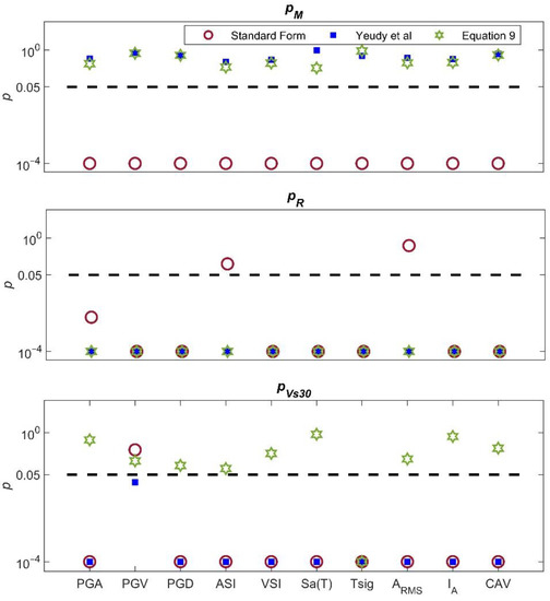
Figure 13.
Sufficiency analysis in terms of p values of different functional forms and IMs. The dotted line marks the p = 0.05 threshold for classifying sufficient (p > 0.05) and insufficient IMs (p < 0.05). Very low p values (p < ) are plotted at p = level. Equation (1) does not show sufficiency with any parameter for most of the analyzed IMs. Equation (24) shows sufficiency only with Mw. Equation (26) shows sufficiency with respect to Mw and Vs30 for most IMs.
With respect to Vs30, the IMs are sufficient for Equation (26) and insufficient for other functional forms. With respect to epicentral distance (Repi), none of the functional forms show sufficiency. This observation contradicts Yeudy’s findings that all the IMs are sufficient (p > 0.05) when using their proposed IM-EDP relation (Equation (24)). This inconsistency may arise from the different near-field ground motion dataset used in their study. While Yeudy’s dataset considers many small magnitude events (Mw < 5) at distances less than 50 km, large events (Mw > 5) dominate our dataset at least up to 100 km. The seismic energy radiated from these larger-magnitude earthquakes has different attenuation behavior with distance, contributing to variations in the predicted EDP. Small magnitude events produce ground motions that attenuate faster at shorter distances, while large events attenuate more gradually over larger distances. To verify, we divide our ground motion dataset into distance bins and calculate pR values (Figure 14). When grouped into distance bins, we observe sufficiency for most IMs in the 30–100 km range.
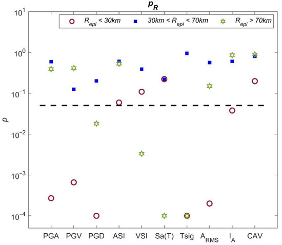
Figure 14.
p values with respect to epicentral distance segregated into bins. When grouped into distance bins, most IMs show sufficiency with respect to epicentral distance for Repi > 30 km.
We now address the role of structural period in the IM-EDP relationship by computing efficiency and sufficiency by adopting Equation (26) for short-period and long-period structures separately. We classify all structures with fundamental periods less than 0.5 s as short-period structures (based on Figure 6a, in which correlations with PGV and PGA at T = 0.5 s are similar) and remaining structures as long-period structures. We skip intermediate-period structures in this analysis because of their similar behavior with longer-period structures. We adopt a combination of IM approaches, similar to vector-valued implementation of IMs proposed by Baker and Cornell [102], and evaluate the efficiency and p values for selected IMs and their combinations as listed in Table 9 and Table 10. We find that the listed IMs are more efficient for short-period structures (Table 9), and that on average, efficiency decreases by 25% for long-period structures (Table 10). A combination of peak measure, PGA, and energy measure, ARMS, results in good efficiency and sufficiency (pM, pR and pVs30) for T < 0.5 s.
Table 9.
Efficiency and p values for frames < 0.5 s.
Table 10.
Efficiency and p values for frames > 0.5 s.
For long-period structures, a combination of IMs is more efficient in the IM-EDP relationship. However, we do not observe sufficiency with respect to epicentral distance (pR) due to the lack of Mw < 5 events in our dataset. A combination of a peak measure, PGV, spectral measure, VSI, and energy measure, ARMS, provides good efficiency and sufficiency (pM and pVs30) for T > 0.5 s.
In summary, these multi-IMs coupled with seismological and structural parameters in the regression model provide an efficient and sufficient prediction of EDPs by IMs. However, a few limitations of our review on ground motion intensity measures and selection techniques need to be mentioned. First, the adopted 2D RC frame models simplify the additional modes of deformations that may include torsional effects. Second, the ground motion duration is likely to impact building response, especially for sites located on top of deep sedimentary structures. However, the building models adopted here do not account for fatigue effects due to long-period cyclic loading. Last, the consideration of a single response measure (ISD, in this case) may not always be sufficient to characterize the complete structural response. Other measures of EDPs, such as hysteretic energy dissipation and co-seismic frequency of structure, should also be investigated in the future.
5. Conclusions and Future Directions
The complexities of the earthquake source process, heterogeneities in 3D Earth structure through which seismic waves travel, and intricate local site conditions govern the response of structures subjected to earthquake shaking. In a PBEE framework, different characteristics of earthquake ground motions, quantified in terms of parameters related to wave amplitude, spectral content, and energy, are represented by a variety of intensity measures (IMs). Several intensity measures are reviewed in this paper, as well as the thought processes behind their development. Following this, we discuss ground motion selection approaches from the basic level to the state of the art with a special focus on IM-based approaches.
Next, based on more than 3500 near-field strong motion recordings (magnitude between Mw 5–8) from the NGA West 2 PEER database and structural analysis of a set of different 2D reinforced concrete frames, we discuss the correlations between ten simple IMs and building response (inter-story drift ratio). The natural period of the structural frames varies from 0.1 to 1.55 sec, and the corresponding building response is extracted by using non-linear time history analysis. We analyze the effect of structural (Tf) and seismological parameters (Mw, Repi, Vs30) on IM-EDP correlations. Finally, we provide recommendations on how to obtain efficient and sufficient EDPs from these IMs.
Seismological and structural uncertainties pose both challenges and opportunities for future research. Despite the improvements in ground motion sensors and the increasing importance of rotational motion on structures in recent studies [103,104], rotational motion is rarely considered in IMs. Researchers have proposed IMs for rocking structures [105,106] that are more susceptible to rotational motion damage, but a broader research effort is needed to develop further IMs.
Recent advances in machine learning have led to the development of innovative approaches for simulating synthetic ground motions [107,108] and developing new ground motion models [109,110,111,112,113]. It may be interesting to apply these novel techniques to evaluating intensity measures and choosing ground motion records. A few studies have used these strategies for determining efficient IMs [114,115] and for proposing new metrics to evaluate IMs [116]. To the best of our knowledge, there are no stand-alone machine learning algorithms for selecting ground motions. With high performance computing capabilities and innovative clustering algorithms, this problem will be addressed in the near future, thus forging the paths for machine-learning-based seismic hazard quantification and earthquake risk mitigation.
Author Contributions
Methodology, T.A.A. and J.S.; Validation, P.M.M.; Formal analysis, T.A.A.; Investigation, T.A.A. and J.S.; Data curation, T.A.A.; Writing—original draft, T.A.A.; Writing—review & editing, J.S. and P.M.M.; Supervision, J.S. and P.M.M. All authors have read and agreed to the published version of the manuscript.
Funding
The research presented in this article is supported by King Abdullah University of Science and Technology (KAUST) in Thuwal, Saudi Arabia, by grant BAS/1/1339-01-01.
Institutional Review Board Statement
Not applicable.
Informed Consent Statement
Not applicable.
Data Availability Statement
The ground motion data used in this study can be downloaded from https://ngawest2.berkeley.edu/, accessed on 25 August 2022.
Conflicts of Interest
The authors declare no conflict of interest.
References
- Baker, J.W.; Cornell, C.A. Uncertainty propagation in probabilistic seismic loss estimation. Struct. Saf. 2008, 30, 236–252. [Google Scholar] [CrossRef]
- Ambraseys, N.N.; Douglas, J.; Sarma, S.K.; Smit, P.M. Equations for the Estimation of Strong Ground Motions from Shallow Crustal Earthquakes Using Data from Europe and the Middle East: Horizontal Peak Ground Acceleration and Spectral Acceleration. Bull. Earthq. Eng. 2005, 3, 1–53. [Google Scholar] [CrossRef]
- Shome, N. Probabilistic Seismic Demand Analysis of Nonlinear Structures. PhD Thesis, Stanford University, Stanford, CA, USA, 1999. [Google Scholar]
- Padgett, J.E.; Nielson, B.G.; DesRoches, R. Selection of optimal intensity measures in probabilistic seismic demand models of highway bridge portfolios. Earthq. Eng. Struct. Dyn. 2008, 37, 711–725. [Google Scholar] [CrossRef]
- Luco, N.; Cornell, C.A. Structure-specific scalar intensity measures for near-source and ordinary earthquake ground motions. Earthq. Spectra 2007, 23, 357–392. [Google Scholar] [CrossRef]
- Vargas-Alzate, Y.F.; Hurtado, J.E.; Pujades, L.G. New insights into the relationship between seismic intensity measures and nonlinear structural response. Bull. Earthq. Eng. 2022, 20, 2365–2395. [Google Scholar] [CrossRef]
- Marafi, N.A.; Berman, J.W.; Eberhard, M.O. Ductility-dependent intensity measure that accounts for ground-motion spectral shape and duration. Earthq. Eng. Struct. Dyn. 2016, 45, 653–672. [Google Scholar] [CrossRef]
- Giovenale, P.; Cornell, C.A.; Esteva, L. Comparing the adequacy of alternative ground motion intensity measures for the estimation of structural responses. Earthq. Eng. Struct. Dyn. 2004, 33, 951–979. [Google Scholar] [CrossRef]
- Gehl, P.; Seyedi, D.M.; Douglas, J. Vector-valued fragility functions for seismic risk evaluation. Bull. Earthq. Eng. 2013, 11, 365–384. [Google Scholar] [CrossRef]
- Elenas, A. Correlation between seismic acceleration parameters and overall structural damage indices of buildings. Soil Dyn. Earthq. Eng. 2000, 20, 93–100. [Google Scholar] [CrossRef]
- Elenas, A.; Meskouris, K. Correlation study between seismic acceleration parameters and damage indices of structures. Eng. Struct. 2001, 23, 698–704. [Google Scholar] [CrossRef]
- Shome, N.; Cornell, C.A.; Bazzurro, P.; Carballo, J.E. Earthquakes, records, and nonlinear responses. Earthq. Spectra 1998, 14, 469–500. [Google Scholar] [CrossRef]
- Alavi, B.; Krawinkler, H. Effects of Near-Fault Ground Motions on Frame Structures; Report No.138; Blume Earthquake Engineering Center: Stanford, CA, USA, 2001. [Google Scholar]
- Clinton, J.F.; Bradford, S.C.; Heaton, T.H.; Favela, J. The observed wander of the natural frequencies in a structure. Bull. Seismol. Soc. Am. 2006, 96, 237–257. [Google Scholar] [CrossRef]
- Krawinkler, H.; Medina, R.; Alavi, B. Seismic drift and ductility demands and their dependence on ground motions. Eng. Struct. 2003, 25, 637–653. [Google Scholar] [CrossRef]
- Luco, N. Probabilistic Seismic Demand Analysis, SMRF Connection Fractures, and Nearsource Effects. Ph.D. Thesis, Department of Civil and Environmental Engineering, Stanford University, Stanford, CA, USA, 2002. [Google Scholar]
- Vamvatsikos, D.; Cornell, C.A. Developing efficient scalar and vector intensity measures for IDA capacity estimation by incorporating elastic spectral shape information. Earthq. Eng. Struct. Dyn. 2005, 34, 1573–1600. [Google Scholar] [CrossRef]
- Weng, Y.-T.; Tsai, K.-C.; Chan, Y.-R. A ground motion scaling method considering higher-mode effects and structural characteristics. Earthq. Spectra 2010, 26, 841–867. [Google Scholar] [CrossRef]
- Yahyaabadi, A.; Tehranizadeh, M. Nonlinear dynamic analysis of structures under near-fault ground motions using an improved scaling method. Asian J. Civ. Eng. 2010, 11, 645–661. [Google Scholar]
- Carballo, J.E.; Cornell, C.A. Probabilistic Seismic Demand Analysis: Spectrum Matching and Design; Report No. RMS-41; RMS Program; Stanford University: Stanford, CA, USA, 2000. [Google Scholar]
- Baker, J.W.; Cornell, C.A. A vector-valued ground motion intensity measure consisting of spectral acceleration and epsilon. Earthq. Eng. Struct. Dyn. 2005, 34, 1193–1217. [Google Scholar] [CrossRef]
- Haselton, C.B.; Baker, J.W. Ground motion intensity measures for collapse capacity prediction: Choice of optimal spectral period and effect of spectral shape. In Proceedings of the 8NCEE, San Francisco, CA, USA, 18–22 April 2006. [Google Scholar]
- Cordova, P.P.; Deierlein, G.G.; Mehanny, S.S.F.; Cornell, C.A. Development of a two-parameter seismic intensity measure and probabilistic assessment procedure. In Proceedings of the 2nd US-Japan Workshop on Performance-based Earthquake Engineering Methodology for RC Building Structures, 11–13 September 2001; pp. 187–206. [Google Scholar]
- Mehanny, S.S.F. A broad-range power-law form scalar-based seismic intensity measure. Eng. Struct. 2009, 31, 1354–1368. [Google Scholar] [CrossRef]
- Lin, L. Development of Improved Intensity Measures for Probabilistic Seismic Demand Analysis. Ph.D. Thesis, Department of Civil Engineering, University of Ottawa, Ottawa, ON, Canada, 2008. [Google Scholar]
- Lin, L.; Naumoski, N.; Saatcioglu, M.; Foo, S. Improved intensity measures for probabilistic seismic demand analysis, Part 1: Development of improved intensity measures. Can. J. Civ. Eng. 2001, 38, 79–88. [Google Scholar] [CrossRef]
- Bianchini, M.; Diotallevi, P.P.; Baker, J.W. Prediction of inelastic structural response using an average of spectral accelerations. In Proceedings of the 10th International Conference On Structural Safety And Reliability (ICOSSAR09), Osaka, Japan, 13–17 September 2009. [Google Scholar]
- Tsantaki, S.; Jäger, C.; Adam, C. Improved seismic collapse prediction of inelastic simple systems vulnerable to the P-delta effect based on average spectral acceleration. In Proceedings of the 15th World Conference on Earthquake Engineering, Lisbon, Portugal, 24–28 September 2012. [Google Scholar]
- Bojorquez, E.; Iervolino, I. A spectral shape-based ground motion intensity measure for maximum and cumulative structural demands. In Proceedings of the European Conference on Earthquake Engineering, Ohrid, Macedonia, 30 August–3 September 2010. [Google Scholar]
- Bojorquez, E.; Iervolino, I. Spectral shape proxies and nonlinear structural response. Soil Dyn. Earthq. Eng. 2011, 31, 996–1008. [Google Scholar] [CrossRef]
- Eads, L.; Miranda, E.; Lignos, D.G. Seismic Collapse Risk Assessment of Buildings: Effects of Intensity Measure Selection and Computational Approach; Report No. 184; The John A. Blume Earthquake Engineering Center, Stanford University: Stanford, CA, USA, 2014. [Google Scholar]
- Eads, L.; Miranda, E.; Lignos, D.G. Average spectral acceleration as an intensity measure for collapse risk assessment. Earthq. Eng. Struct. Dyn. 2015, 44, 2057–2073. [Google Scholar] [CrossRef]
- Xiao, L.U.; LiePing, Y.E.; XinZheng, L.U.; MengKe, L.I.; XiaoWei, M.A. An improved ground motion intensity measure for super high-rise buildings. Sci. China 2013, 56, 1525–1533. [Google Scholar]
- Xiao, L.U.; XinZheng, L.U.; LiePing, Y.E.; MengKe, L.I. Development of an improved ground motion intensity measure for super high-rise buildings. J. Build. Struct. 2014, 35, 15–21. [Google Scholar]
- Yahyaabadi, A.; Tehranizadeh, M. Introducing a new scaling method for near-fault ground motions based on the root-mean-square of spectral responses. In Proceedings of the ECCOMAS Thematic Conference on Computational Methods in Structural Dynamics and earthquake Engineering, Corfu Island, Greece, 25–28 May 2011. [Google Scholar]
- Housner, G.W. Spectrum intensity of strong-motion earthquakes. In Proceedings of the Symposium on Earthquakes and Blast Effects on Structures, EERI, Los Angeles, CA, USA, 10 October 2016. [Google Scholar]
- Von Thun, J.L.; Rochim, L.H.; Scott, G.A.; Wilson, J.A. Earthquake ground motions for design and analysis of dams. In Earthquake Engineering and Soil Dynamics II—Recent Advances in Ground-Motion Evaluation (Geotechnical Special Publication 20); ASCE: New York, NY, USA, 1988; pp. 463–481. [Google Scholar]
- Kappos, A.J. Sensitivity of calculated inelastic seismic response to input motion characteristics. In Proceedings of the 4th National Conference on Earthquake Engineering, Palm Springs, CA, USA, 20–24 May 1990; Volume 2, pp. 25–34. [Google Scholar]
- Matsumura, K. On the intensity measure of strong motion related to structural failures. In Proceedings of the 10th World Conference on Earthquake Engineering, Rotterdam, The Netherlands, 19–24 July 1992; pp. 375–380. [Google Scholar]
- Martinez-Rueda, J.E. Scaling procedure for natural accelerograms based on a system of spectrum intensity scales. Earthq. Spectra 1998, 14, 135–152. [Google Scholar] [CrossRef]
- Bommer, J.J.; Martinez-Pereira, A. The effective duration of earthquake strong motion. J. Earthq. Eng. 1999, 3, 127–172. [Google Scholar] [CrossRef]
- Bommer, J.J.; Magenes, G.; Hancock, J.; Penazzo, P. The influence of strong-motion duration on the seismic response of masonry structures. Bull. Earthq. Eng. 2004, 2, 1–26. [Google Scholar] [CrossRef]
- Chandramohan, R.; Baker, J.W.; Deierlein, G.G. Quantifying the Influence of Ground Motion Duration on Structural Collapse Capacity Using Spectrally Equivalent Records. Earthq. Spectra 2016, 32, 927–950. [Google Scholar] [CrossRef]
- Arias, A. Measure of Earthquake Intensity. Seismic Design for Nuclear Power Plants; Hansen, R.J., Ed.; Massachusetts Institute of Technology Press: Cambridge, MA, USA, 1970; pp. 438–483. [Google Scholar]
- Uang, C.M.; Bertero, V.V. Evaluation of seismic energy in structures. Earthq. Eng. Struct. Dyn. 1990, 19, 77–90. [Google Scholar] [CrossRef]
- Housner, G.W. Limit design of structures to resist earthquakes. In Proceedings of the First World Conference on Earthquake Engineering, Berkeley, CA, USA; 1956; pp. 1–12. Available online: https://www.iitk.ac.in/nicee/wcee/article/1_5-1.pdf (accessed on 25 August 2021).
- Elefante, L.; Jalayer, F.; Iervolino, I.; Manfredi, G. Disaggregation-based response weighting scheme for seismic risk assessment of structures. Soil Dyn. Earthq. Eng. 2010, 30, 1513–1527. [Google Scholar] [CrossRef]
- Baker, J.W.; Cornell, C.A. Spectral shape, epsilon and record selection. Earthq. Eng. Struct. Dyn. 2006, 35, 1077–1095. [Google Scholar] [CrossRef]
- Bojórquez, E.; Iervolino, I.; Reyes-Salazar, A.; Ruiz, S.E. Comparing vector-valued intensity measures for fragility analysis of steel frames in the case of narrow-band ground motions. Eng. Struct. 2012, 45, 472–480. [Google Scholar] [CrossRef]
- Theophilou, A.I.; Chryssanthopoulos, M.K.; Kappos, A.J. A vector-valued ground motion intensity measure incorporating normalized spectral area. Bull. Earthq. Eng. 2017, 15, 249–270. [Google Scholar] [CrossRef]
- Perrault, M.; Guéguen, P. Correlation between Ground Motion and Building Response using California Earthquake Records. Earthq. Spectra 2015, 31, 2027–2046. [Google Scholar] [CrossRef]
- Astorga, A.; Guéguen, P.; Ghimire, S.; Kashima, T. NDE1. 0: A new database of earthquake data recordings from buildings for engineering applications. Bull. Earthq. Eng. 2020, 18, 1321–1344. [Google Scholar] [CrossRef]
- Erdik, M.; Apaydın, N. Earthquake response of suspension bridges. In Vibration problems ICOVP 2005; Inan, E., Kiris, A., Eds.; Springer: Berlin/Heidelberg, Germany, 2007. [Google Scholar]
- Mai, P.M. Ground Motion: Complexity and Scaling in the Near Field of Earthquake Ruptures. In Encyclopedia of Complexity and Systems Science; Lee, W.H.K., Meyers, R., Eds.; Springer: Berlin/Heidelberg, Germany, 2009; pp. 4435–4474. [Google Scholar]
- Krinitzsky, E.L. Deterministic versus probabilistic seismic hazard analysis for critical structures. Int. J. Eng. Geol. 1995, 40, 1–7. [Google Scholar] [CrossRef]
- Romeo, R.; Prestininzi, A. Probabilistic versus deterministic seismic hazard analysis: An integrated approach for siting problems. Soil Dyn. Earthq. Eng. 2000, 20, 75–84. [Google Scholar] [CrossRef]
- Cornell, C.A. Engineering seismic risk analysis. Bull. Seismol. Soc. Am. 1968, 58, 1583–1606. [Google Scholar] [CrossRef]
- Algrmissen, S.T.; Perkins, D.M.; Thenhaus, P.C.; Hanson, S.L.; Bender, B.L. Probabilistic estimates of maximum acceleration and velocity in rock in the contiguous United States. In U.S. Geological Survey. Open-File Report 82-1033; US Geological Survey: Washington, DC, USA, 1982. [Google Scholar]
- Reiter, L. Earthquake Hazard Analysis—Issues and Insights; Columbia University Press: New York, NY, USA, 1990. [Google Scholar]
- Anderson, J.G.; Trifunac, M.D. Uniform risk functionals for characterization strong earthquake ground motion. Bull. Seismol. Soc. Am. 1978, 68, 205–218. [Google Scholar]
- Krinitzsky, E.L. The hazard in using probabilistic seismic hazard analysis for critical structures. In Geotechnical earthquake engineering and soil III; Dakoulas, P., Yougain, M., Holtz, R.D., Eds.; ASCE Geotechnical Special Publication: Reston, VA, USA, 1998; Volume 75, p. 1998. [Google Scholar]
- Youngs, R.R.; Power, M.S.; Chin, C.C. Design ground library. In Proceedings of the 8th National Conference on Earthquake Engineering, San Francisco, CA, USA, 18–22 April 2006; p. 893. [Google Scholar]
- Bommer, J.J.; Acevedo, A. The use of real earthquake accelerograms as input to dynamic analysis. J. Earthq. Eng. 2004, 8, 43–91. [Google Scholar] [CrossRef]
- Stewart, J.P.; Chiou, S.J.; Bray, R.W.; Graves, P.; Somerville, G.; Abrahamson, N.A. Ground Motion Evaluation Procedures for Performance-Based Design; PEER report 2001/09; Pacific Earthquake Engineering Research Center, University of California: Berkeley, CA, USA, 2001. [Google Scholar]
- Iervolino, I.; Cornell, C.A. Record selection for nonlinear seismic analysis of structures. Earthq. Spectra 2005, 21, 685–713. [Google Scholar] [CrossRef]
- Bazzurro, P.; Cornell, C.A. Seismic hazard analysis of nonlinear structures, I: Methodology. J. Struct. Eng. ASCE 1994, 120, 3320–3344. [Google Scholar] [CrossRef]
- Bazzurro, P.; Cornell, C.A. Seismic hazard analysis of nonlinear structures, II: Applications. J. Struct. Eng. ASCE 1994, 120, 3345–3365. [Google Scholar] [CrossRef]
- Bommer, J.J.; Scott, S.G. The feasibility of using real accelerograms for seismic design. In Implications of Recent Earthquakes on Seismic Risk; Elnashai, A.S., Antoniou, S., Eds.; Imperial College: London, UK, 2000; Chapter 9. [Google Scholar]
- ASCE Standard No. 004-98; Seismic Analysis of Safety-Related Nuclear Structures and Commentary. American Society of Civil Engineers: Reston, VA, USA, 2000.
- Kawaga, T.; Irikura, K.; Somerville, G.P. Differences in ground motion and fault process between the surface and buried rupture earthquakes. Earth Planets Space 2004, 56, 3–14. [Google Scholar] [CrossRef]
- Lin, P.-S.; Lee, C.-T. Ground-motion attenuation relationships for subductionzone earthquakes in Northeastern Taiwan. Bull. Seismol. Soc. Am. 2008, 98, 220–240. [Google Scholar] [CrossRef]
- Boore, D.M.; Atkinson, G.M. Boore–Atkinson NGA Ground Motion Relations for the Geometric Mean Horizontal Component of Peak and Spectral Ground Motion Parameters; PEER Report 2007/01; Pacific Earthquake Engineering Research Center: Berkeley, CA, USA, 2007. [Google Scholar]
- Stafford, J.P.; Strasser, O.F.; Bommer, J.J. An evaluation of the applicability of the NGA models to ground-motion prediction in the Euro-Mediterranean region. Bull. Earthq. Eng. 2008, 6, 149–177. [Google Scholar] [CrossRef]
- Ambraseys, N.N.; Douglas, J.; Rinaldis, D.; Berge-Thierry, C.; Suhadolc, P.; Costa, G.; Sigbjornsson, R.; Smit, P. Dissemination of European Strong-Motion Data, Vol. 2, CD-ROM Collection; Engineering and Physical Sciences Research Council: Swindon, UK, 2004. [Google Scholar]
- Iervolino, I.; Galasso, C.; Cosenza, E. REXEL: Computer aided record selection for code-based seismic structural analysis. Bull. Earthq. Eng. 2009, 8, 339–362. [Google Scholar] [CrossRef]
- Beyer, K.; Bommer, J.J. Selection and scaling of real accelerograms for bidirectional loading: A review of current practice and code provisions. J. Earthq. Eng. 2007, 11, 13–45. [Google Scholar] [CrossRef]
- Abrahamson, N.A.; Silva, W.J. Empirical response spectral attenuation relations for shallow crustal earthquakes. Seismol. Res. Lett. 1997, 68, 94–126. [Google Scholar] [CrossRef]
- Baker, J.W. Conditional mean spectrum: Tool for ground motion selection. J. Struct. Eng. 2011, 137, 322–331. [Google Scholar] [CrossRef]
- Baker, J.W.; Jayaram, N. Correlation of spectral acceleration values from NGA ground motion models. Earthq. Spectra 2008, 24, 299–317. [Google Scholar] [CrossRef]
- Jayaram, N.; Lin, T.; Baker, J.W. A computationally efficient ground-motion selection algorithm for matching a target response spectrum mean and variance. Earthq. Spectra 2011, 27, 797–815. [Google Scholar] [CrossRef]
- Baker, J.W.; Lee, C. An Improved Algorithm for Selecting Ground Motions to Match a Conditional Spectrum. J. Earthq. Eng. 2018, 22, 708–723. [Google Scholar] [CrossRef]
- Kwong, N.S.; Jaiswal, K.S.; Luco, N.; Baker, J.W. Selecting three components of ground motions from Conditional Spectra for multiple stripe analyses. In Proceedings of the 17th World Conference on Earthquake Engineering, Sendai, Japan, 13–18 September 2020. [Google Scholar]
- Bradley, B.A. A generalized conditional intensity measure approach and holistic groundmotion selection. Earthq. Eng. Struct. Dyn. 2010, 39, 1321–1342. [Google Scholar]
- Bradley, B.A. A ground motion selection algorithm based on the generalized conditional intensity measure approach. Soil Dyn. Earthq. Eng. 2012, 40, 48–61. [Google Scholar] [CrossRef]
- Lin, T.; Harmsen, S.C.; Baker, J.W.; Luco, N. Conditional spectrum computation incorporating multiple causal earthquakes and ground motion prediction models. Bull. Seismol. Soc. Am. 2013, 103, 1103–1116. [Google Scholar] [CrossRef]
- Ha, S.J.; Han, S.W. A method for selecting ground motions that considers target response spectrum mean and variance as well as correlation structure. J. Earthq. Eng. 2016, 20, 1263–1277. [Google Scholar] [CrossRef]
- Bijelić, N.; Lin, T.; Deierlein, G. Validation of the SCEC broadband platform simulations for tall building risk assessments considering spectral shape and duration of the ground motion. Earthq. Eng. Struct. Dynam. 2018, 47, 2233–2251. [Google Scholar] [CrossRef]
- Kohrangi, M.; Vamvatsikos, D.; Bazzurro, P. Multi-level conditional spectrum-based record selection for IDA. Earthq. Spectra. 2020, 36, 1976–1994. [Google Scholar] [CrossRef]
- Kohrangi, M.; Bazzurro, P.; Vamvatsikos, D.; Spillatura, A. Conditional spectrum-based ground motion record selection using average spectral acceleration. Earthq. Eng. Struct. Dyn. 2017, 46, 1667–1685. [Google Scholar] [CrossRef]
- Tarbali, K.; Bradley, B.A. The effect of causal parameter bounds in PSHA-based ground motion selection. Earthq. Eng. Struct. Dyn. 2016, 45, 1515–1535. [Google Scholar] [CrossRef]
- Spillatura, A.; Kohrangi, M.; Bazzurro, P.; Vamvatsikos, D. Conditional spectrum record selection faithful to causative earthquake parameter distributions. Earthq. Engng. Struct. Dyn. 2021, 50, 2653–2671. [Google Scholar] [CrossRef]
- IBC-2009; International Building Code. International Code Council: Country Club Hills, IL, USA, 2009.
- Yassin, M.H.M. Nonlinear Analysis of Prestressed Concrete Sructures under Monotonic and Cyclic Loads; University of California: Berkeley, CA, USA, 1994. [Google Scholar]
- McKenna, F. OpenSees: A framework for earthquake engineering simulation. Comput. Sci. Eng. 2011, 13, 58–66. [Google Scholar] [CrossRef]
- Newmark Nathan, M. A Method of Computation for Structural Dynamics. Trans. Am. Soc. Civ. Eng. 1962, 127, 1406–1433. [Google Scholar] [CrossRef]
- Daneshjoo, F.; Gerami, M. Higher Mode Effects on Seismic Behavior of MDOF Steel Moment Resisting Frames. J. Seismol. Earthq. Eng. 2003, 5, 41–54. [Google Scholar]
- FEMA. Earthquake loss estimation methodology—HAZUS 99; Federal Emergency Management Agency and National Institute of Buildings Sciences: Washington, DC, USA, 1999.
- Cao, V.V.; Ronagh, H.R. Correlation between seismic parameters of far-fault motions and damage indices of low-rise reinforced concrete frames. Soil Dyn. Earthq. Eng. 2014, 66, 102–112. [Google Scholar] [CrossRef]
- Chandramohan, R.; Lin, T.; Baker, J.; Deierlein, G.G. Influence of Ground Motion Spectral Shape and Duration on Seismic Collapse Risk. In Proceedings of the 10th International Conference on Urban Earthquake Engineering, Tokyo, Japan, 1–2 March 2013. [Google Scholar]
- Dutta, A.; Mander, J.B. Energy Based Methodology for Ductile Design of Concrete Columns. J. Struct. Eng. 2001, 127, 1374–1381. [Google Scholar] [CrossRef]
- Ozmen, H.; Inel, M. Damage potential of earthquake records for RC building stock. Earthq. Struct. 2016, 10, 1315–1330. [Google Scholar] [CrossRef]
- Baker, J.W.; Cornell, C.A. Vector-valued Intensity Measures Incorporating Spectral Shape For Prediction of Structural Response. J. Earthq. Eng. 2008, 12, 534–554. [Google Scholar] [CrossRef]
- Trifunac, M.D. A note on rotational components of earthquake motions on ground surface for incident body waves. Soil Dyn. Earthq. Eng. 1982, 1, 11–19. [Google Scholar] [CrossRef]
- Trifunac, M.D. Effects of torsional and rocking excitations on the response of structures. In Earthquake Source Asymmetry, Structural Media and Rotation Effects; Teisseyre, R., Ed.; Springer: Heidelberg, Germany, 2006; pp. 569–582. [Google Scholar]
- Shokrabadi, M.; Burton, H.V. Ground Motion Intensity Measures for Rocking Building Systems. Earthq. Spectra 2017, 33, 1533–1554. [Google Scholar] [CrossRef]
- Kavvadias, I.E.; Papachatzakis, G.A.; Bantilas, K.E.; Vasiliadis, L.K.; Elenas, A. Rocking spectrum intensity measures for seismic assessment of rocking rigid blocks. Soil Dyn. Earthq. Eng. 2017, 101, 116–124. [Google Scholar] [CrossRef]
- Paolucci, R.; Gatti, F.; Infantino, M.; Smerzini, C.; Ozcebe, A.G.; Stupazzini, M. Broadband Ground Motions from 3D Physics-Based Numerical Simulations Using Artificial Neural Networks. Bull. Seism. Soc. Am. 2018, 108, 1272–1286. [Google Scholar] [CrossRef]
- Okazaki, T.; Hachiya, H.; Iwaki, A.; Maeda, T.; Fujiwara, H.; Ueda, N. Simulation of broad-band ground motions with consistent long-period and short-period components using the Wasserstein interpolation of acceleration envelopes. Geophys. J. Int. 2021, 227, 333–349. [Google Scholar] [CrossRef]
- Derras, B.; Bard, P.Y.; Cotton, F.; Bekkouche, A. Adapting the neural network approach to PGA prediction: An example based on the KiK-net data. Bull. Seismol. Soc. Am. 2012, 102, 1446–1461. [Google Scholar] [CrossRef]
- Derras, B.; Bard, P.Y.; Cotton, F. Towards fully data driven ground motion prediction models for Europe. Bull. Earthq. Eng. 2014, 12, 495–516. [Google Scholar] [CrossRef]
- Derras, B.; Bard, P.Y.; Cotton, F. Site-conditions proxies, ground-motion variability and data-driven GMPEs: Insights from NGA-West 2 and RESORCE data sets. Earthq. Spectra 2016, 32, 2027–2056. [Google Scholar] [CrossRef]
- Trugman, D.T.; Shearer, P.M. Strong Correlation between stress drop and peak ground acceleration for recent M 1–4 earthquakes in the San Francisco Bay Area. Bull. Seismol. Soc. Am. 2018, 108, 929–945. [Google Scholar] [CrossRef]
- Farid, K.; Patricia, C. Machine learning in ground motion prediction. Comput. Geosci. 2021, 148, 104700. [Google Scholar] [CrossRef]
- Bijelić, N.; Lin, T.; Deierlein, G.G. Efficient intensity measures and machine learning algorithms for collapse prediction of tall buildings informed by SCEC CyberShake ground motion simulations. Earthq. Spectra. 2020, 36, 1188–1207. [Google Scholar] [CrossRef]
- Xu, Y.; Lu, X.; Tian, Y.; Huang, Y. Real-Time Seismic Damage Prediction and Comparison of Various Ground Motion Intensity Measures Based on Machine Learning. J. Earthq. Eng. 2022, 26, 4259–4279. [Google Scholar] [CrossRef]
- Yan, Y.; Xia, Y.; Yang, J.; Sun, L. Optimal selection of scalar and vector-valued seismic intensity measures based on Gaussian Process Regression. Soil Dyn. Earthq. Eng. 2022, 152, 106961. [Google Scholar] [CrossRef]
Publisher’s Note: MDPI stays neutral with regard to jurisdictional claims in published maps and institutional affiliations. |
© 2022 by the authors. Licensee MDPI, Basel, Switzerland. This article is an open access article distributed under the terms and conditions of the Creative Commons Attribution (CC BY) license (https://creativecommons.org/licenses/by/4.0/).