Featured Application
This article belongs to the Section Computing and Artificial Intelligence.
Abstract
Ineffective protein feature representation poses problems in protein classification in hierarchical structures. Discrete wavelet transform (DWT) is a feature representation method which generates global and local features based on different wavelet families and decomposition levels. To represent protein sequences, the proper wavelet family and decomposition level must be selected. This paper proposed a hybrid optimization method using particle swarm optimization and the firefly algorithm (FAPSO) to choose the suitable wavelet family and decomposition level of wavelet transformation for protein feature representation. The suggested approach improved on the work of earlier researchers who, in most cases, manually selected the wavelet family and level of decomposition based solely on experience and not on data. The paper also applied the virtual class methods to overcome the error propagation problems in hierarchical classification. The effectiveness of the proposed method was tested on a G-Protein Coupled Receptor (GPCR) protein data set consisting of 5 classes at the family level, 38 classes at the subfamily level, and 87 classes at the sub-subfamily level. Based on the result obtained, the most selected wavelet family and decomposition level chosen to represent GPCR classes by FAPSO are Biorthogonal wavelets and decomposition level 1, respectively. The experimental results show that the representation of GPCR protein using the FAPSO algorithm with virtual classes can yield 97.9%, 86.9%, and 81.3% classification accuracy at the family, subfamily, and sub-subfamily levels, respectively. In conclusion, the result shows that the selection of optimized wavelet family and decomposition level by the FAPSO algorithm, and the virtual class method can be potentially used as the feature representation method and a hierarchical classification method for GPCR protein.
1. Introduction
Labeling data according to classes in a hierarchy is also known as hierarchical classification. Most real data can be classified as hierarchical classifications, in areas as disparate as diseases, text, visuals, plant species, protein functions, websites, documentation, music genres, and images. Manually labeling real data in a hierarchical structure is challenging and complex. In addition, the hierarchical classification problem becomes more difficult as the amount of data increases over time. Although many classification methods have been developed to automate the classification task, these methods are inefficient and ineffective for hierarchical classification. This is because these methods ignore the relationship information between classes in a hierarchy [1]. Various methods have been introduced to overcome the weaknesses of hierarchical classification methods in past studies. However, there is still room to improve existing methods by conducting various experiments related to hierarchical classification.
One of the ways to overcome the problem of hierarchical classification is to consider the feature representation of each class in the hierarchy. Each feature has a different level of relevance to represent each class in the hierarchy [2]. The use of inappropriate features may affect the performance of classification [3,4]. There are many different feature representation techniques used to represent protein sequences. The well-known amino acid composition (AAC) feature representation method represents protein classes based on the number of amino acids in the protein sequence. However, this AAC method has the disadvantage that it does not contain protein sequence information [3]. This problem is overcome by the pseudo amino acid composition (PseAAC) feature representation method. The PseAAC feature representation method can convert protein features based on the number of amino acids and contains information on the order of amino acids in the protein sequence [5]. There are additional protein feature representation methods such as N-gram [6,7], position-specific scoring matrix (PSSM) [8,9], z- value [10], and a combination of several features [11]. According to [12,13], most studies use global features with the entire protein sequence information for protein representation. Nevertheless, these global features cannot extract hidden information in protein sequences [13]. In addition, global features contain overlapping and unnecessary information [11,14].
Discrete wavelet transform (DWT) is a feature representation method that has the ability to perform analysis at various levels [15,16,17]. The DWT method is suitable for representing features of biological data [13,16,17,18,19]. With the property of multiresolution analysis, DWT can provide information on protein sequence arrangement more effectively and allow biological signals to be analyzed in the frequency domain and time domain [17,19]. This differs from signal processing methods such as Fourier transform, which can only study signals in the frequency domain [13,15,20,21]. Therefore, the DWT method can provide more information compared to other feature representation methods [22,23,24,25]. DWT can produce global features and local features in various decomposition levels to be analyzed, and produce features that do not have overlaps [26]. Global features are obtained from approximation DWT coefficients, while local features are obtained from detailed DWT coefficients [17].
Despite many advantages of DWT, the main problem is selecting the appropriate DWT family type and decomposition level to represent each class in the GPCR protein hierarchy. Different types of families and decomposition levels can be used in DWT. The appropriate DWT family type and decomposition level selection are important in data analysis because an accurate representation will preserve the data’s important characteristics [27,28,29]. Furthermore, it assists in understanding the organization and complexity of this data [16,30]. The selected DWT family needs to meet the characteristics of orthogonality, symmetry, and shape similarity with the studied data [31,32]. The application type impacts the wavelet chosen, and out-of-range decomposition levels produce useless data, which harms data analysis [33]. Furthermore, the selection of the appropriate family type and DWT decomposition level for the feature representation of a class is important because these two parameters affect the classification performance [34,35,36]. However, previous studies have mostly selected the DWT family type and decomposition level, based on experience or manually [4,30]. They did not find the optimal wavelet family and decomposition level based on the data used. The well-known DWT families include Haar, Daubechies, Coiflets, Symlets, Discrete Meyer, and Biorthogonal. The differences between these DWT families include compact size, vanishing moment, symmetry, and orthogonality [37]. The decomposition level is related to the number of global and local features produced from DWT [34]. Using a high level of decomposition on a short sequence will create overlapping information, while using a low decomposition level on a long sequence will ignore much information.
Some studies use metaheuristic methods to optimize the selection of DWT family types and decomposition levels such as genetic algorithms [27,38], particle swarm optimization [27,34,39], whale optimization algorithm [28] and evolutionary quantum crowding [29]. However, no research has been performed to choose the optimal DWT family type and decomposition level for protein feature representation in hierarchical classes. This study uses a hybrid optimization method between the particle swarm optimization algorithm and the firefly algorithm (FAPSO) to select DWT’s family and decomposition level. This hybridization is necessary to overcome the shortcomings of particle swarm optimization (PSO) and firefly algorithm (FA) algorithms [40]. The PSO algorithm has several weaknesses such as premature convergence or being trapped in local optima and a low convergence rate in the exploitation process [41,42]. The FA algorithm has advantages compared to the PSO algorithm, such as no local and global parameters which could prevent it from getting stuck in local minima and premature convergence. In addition, the FA algorithm does not have a velocity parameter that can overcome the problem of the slowness of a particle’s velocity. In this study, FA and PSO algorithms have been combined to prevent premature convergence of each algorithm, avoid local optima, and balance the exploitation and exploration processes [43].
The other problem relates to error propagation in hierarchical classification. It is a classification error in the nodes at the top level of the hierarchy. Then, this classification error will continue to the bottom level of the hierarchy and affect the classification results. This error propagation cannot be corrected at the bottom of the hierarchy [44,45]. There are various methods to overcome the error propagation problem in hierarchical classification [22,45,46,47]. This study used the virtual class method introduced by [48] to overcome this problem. This method was also used in [49] to overcome the problem of propagation errors in text hierarchy classification. In this method, each parent node except the root node and the terminal node will have one child node known as the virtual class node. These virtual nodes contain the training data from the parent node only. During the training phase, each classification model on each parent node will learn how to classify data only between the node and the virtual class node. The models generated at each parent node use the top-down classification method during the testing phase. A study by [49] found that this virtual class method can avoid the problem of propagated error by stopping the classification at the correct hierarchical level. This method can produce good experimental results compared to the hierarchical classification method by overcoming the problem of error propagation.
Therefore, this study analyzes the suitable wavelet family and decomposition level using the FAPSO optimization method and utilizing virtual classes for GPCR hierarchical protein classification.
2. G-Protein Coupled Receptor
G protein-coupled receptors (GPCR) exist on the surface of every cell [50]. GPCRs generate signals in cells to regulate key physiological processes such as hormone signalling, neurotransmission, cognition, vision, taste, pain perception, and others. It is also known as the seven transmembrane domain (7TM) receptor, because there are seven transmembrane segments in which three loops are outside the cell, and three loops are inside the cell with the N-terminal position being inside the cell and the C-terminal being outside the cell. GPCR hierarchy consists of three levels, namely family, subfamily, and sub-subfamily. The family class consists of five classes, namely families A, B, C, D, and E. The subfamily class consists of 38 classes, and the sub-subfamily class consists of 87 classes. Since there are very complex relationships between classes, GPCR classification has proven difficult [51]. In addition, many protein sequences in the same family share homology with protein sequences in other families, which also increases the difficulty of classification [52]. GPCR classification depends on sequence order and includes structural, functional, and evolutionary characteristics, such as chemical and pharmacological factors [53]. GPCRs are thus one of the most challenging datasets to classify.
Various feature representation methods have been used in past research for GPCR proteins. Ref. [3] used the amino acid composition (AAC), pseudo amino acid composition (PseAAC), and dipeptide composition (DC) feature representation methods for the classification of GPCR proteins. Ref. [54] used several indices related to the hydrophobicity of amino acids to implicitly describe the properties of protein sequences. They showed that combining three hydrophobic indices with a constrained Boltzmann machine (RBM) achieved high-performance results for class C GPCR classification with 94% accuracy. The Ngram representation method was used by [6,55] to represent GPCR proteins.
The Local Descriptor feature representation method has been used by [52]. This representation method works by grouping amino acids into three groups: hydrophobic, neutral, and polar. This method has yielded 87% to 90% accuracy for the GPCR protein hierarchy family level.
Deep learning methods have been used for GPCR protein classification by [51,55,56,57]. The feature representation method and deep learning design varied between these studies. Ref. [51] used a combination of the n-gram feature representation method, term frequency-inverse document frequency (TF-IDF), and deep learning. This study has obtained an accuracy of 98.5% at the family level, 98.1% at the subfamily level, and 96.4% at the sub-subfamily level. Ref. [57] have used the deep learning method with one-hot coding feature representation and achieved an accuracy of 97.17% for the family level, 86.82% for the subfamily level and 81.17% for the sub-subfamily level. Ref. [55] used 1-2-3-g feature representation in deep learning methods and achieved an accuracy of 99.2% for the family level, 99.2% for the subfamily level, and 98.15% for the sub-subfamily level. Ref. [56] has used 2-3-4 g feature representation together with deep learning and obtained an accuracy of 97.40% for the family level, 87.78% for the subfamily level, and 81.13% for the sub-subfamily level. However, the performance of these studies cannot be directly compared because studies used different GPCR datasets.
Ref. [58] used the DWT method and selected the DWT Coiflet 4 family with three levels of decomposition to represent GPCR protein features for the levels of family A, B and C, subfamily A, as well as sub-subfamily Amine. This study found that the Coiflet 4 family type had the highest accuracies compared to other DWT families, which is 99.67% for the family level, 97.64% for the A subfamily, and 99.20% for the Amine sub-subfamily. Ref. [59] used Fourier transform for GPCR protein classification. That study produced an accuracy of 96.1% for the classification of GPCR proteins at the family level.
Several feature representation methods have been combined to represent GPCR proteins. Ref. [7] combined the 400D feature representation method and parallel correlation pseudo amino acid composition (PC-PseAAC). Ref. [60] has produced 1497 features as a result of a combination of AAC feature representation, PseAAC, dipeptide composition, correlation feature, composition, transition, distribution, and sequence arrangement. Ref. [61] combined PseAAC, AAC, and dipeptide decomposition feature representation methods to obtain high classification performance. Ref. [62] hybridized PseAAC feature and energy from DWT approximation coefficients and detail to represent protein classes at three levels of the GPCR protein hierarchy. It was found that combining several feature representation methods could produce better classification performance as compared to the use of individual feature representation methods.
3. The Procedures of Protein Feature Representation and Classification
This work proposes an approach to classifying GPCR protein based on the discrete wavelet transform optimal features produced by the hybridization of the firefly algorithm and particle swarm optimization (FAPSO). In addition, the virtual class (VC) method is utilized in GPCR hierarchical protein classification. The following subsection will describe the procedures involved in this study.
3.1. Data Collection
The G-Protein Coupled Receptor (GPCR) protein hierarchy benchmark dataset, often known as GDS, is used in this study. The length of each protein sequence does not exceed 280 residues. Only classes with more than ten data at the third hierarchical level are used, with a total of 5 classes at the first level, 36 classes at the second level, and 87 classes at the third level. In total, 8222 protein sequences were used in this study. The GDS dataset can be found at http://www.cs.kent.ac.uk/projects/biasprofs/downloads.html, accessed on 23 March 2014. Numerous studies, including [2,57,61,63,64,65], have used this dataset.
3.2. Feature Representation
The GPCR protein sequences are initially represented using the pseudo amino acid composition (PseAAC) method. With this method, the protein sequences are transformed into numeric. The following steps are taken to convert protein sequences to numerical features using the PseAAC method. Protein P can be written as follows in the PseAAC method:
where
PseAAC = P1, P2,..., P20,..., P^,
The frequency of amino acids in the sequence is represented by the first twenty elements in Equation (1), from P1 to P20. The amino acid correlation rank is represented by the symbol λ where λ = 1,…, m. This rank value is an integer that is non-negative and less than the length of the protein sequence. The number of physiochemical characteristics of the amino acid employed is represented by the n value. This study used the same six physiochemical properties of amino acids as [66], namely the mass properties, the pK group from pK from the α-COOH group, and the pI group at 25 °C. The weighting factor w was made to put more weight on PseAAC than amino acid composition. PseAAC features can be retrieved from the PseAAC web server [67]. There are two different kinds of PseAAC, type I and type II. Researchers [66] found that PseAAC type II works better as a protein feature. This is because, unlike type I PseAAC, type II PseAAC takes into account the impact of physiochemical characteristics in the calculation [68]. According to Equation (2), the total number of features created for each protein sequence based on the parameters determined above is =20 + 6 25, or 170 features.
Following that, the PseAAC features are normalised, with each feature scaled to the limit range [0, 1] so that the feature value is in a small range. Normalising features prevents large values from dominating small values. Additionally, this helps simplify the computation process. The formula for feature normalisation is in Equation (3):
where is the value of the feature after the normalisation process, is the original value of the feature, and are the maximum value and minimum value of the entire features.
The wavelet transform is then calculated using the normalised PseAAC features. The scaling function and the wavelet function are the two most important functions in DWT. Using the scaling function, it is possible to obtain low-frequency features for the normalised PseAAC. Approximation coefficients are low-frequency features that contain global information. The definition of the scaling function is as in Equation (4) [69]:
where x, a, and b denote the data, scaling, and translation parameters, respectively. To obtain detail coefficients or local features, the wavelet function is used. The definition of the wavelet function is in Equation (5) [69]:
where x, a, and b denote the data, scaling, and translation parameters, respectively. To form the coefficient vector, both approximation and detail coefficients are combined depending on the wavelet family and decomposition level chosen. The detail coefficients are maintained in this study because they may provide useful information.
Different wavelet family types can be used to implement DWT. Scaling and wavelet functions differ for each type of wavelet family [34]. It is essential to choose the right kind of family in order to make effective use of DWT [70]. In this particular research, there are 82 different wavelet families that can be used to describe GPCR proteins. This wavelet family includes 20 from the Daubechies family (Db1-Db20); 20 from the Symlet family (Sym1-Sym20); 5 from the Coiflet family (Coif1-Coif5); 6 from the Fejer–Korovkin family; 15 from the Biorthogonal family; 15 from the Reverse Biorthogonal family; and 1 from the Meyer family. Each family is distinguished by its compact support, vanishing moment, symmetry, and orthogonality [71].
The DWT is also capable of analysing PseAAC feature vectors at many resolutions. This can be accomplished by breaking down the PseAAC feature vector into different levels of decomposition. The utmost decomposition level that can be implemented is determined by the formula log2 (N), where N is the PseAAC feature size. Considering PseAAC has 170 features, the maximum potential decomposition is 7 levels.
3.3. Hybrid Particle Swarm Optimization Algorithm and Firefly Algorithm (FAPSO)
The selection of the wavelet family and decomposition level suitable for each protein class is important because it can produce better features and information [72]. This study uses a hybrid algorithm between PSO and FA to obtain the optimal wavelet family and decomposition level to represent GPCR protein class features.
This hybrid algorithm was introduced by [43] to improve the local search mechanism based on the best global parameters from previous studies. This objective can be achieved by exploiting the advantages of these two algorithms. The particle swarm optimization (PSO) algorithm is used in global search and produces fast convergence in the exploration process. Meanwhile, the firefly algorithm (FA) is used in the local search process because it can fine-tune the exploitation process.
Initially, the parameters used in both algorithms are given default values as in Table 1. Next, the particles choose the wavelet family and decomposition level from the 82 wavelet families and 7 decomposition levels. The wavelet features will be generated based on the value of the wavelet family and the decomposition level. In this algorithm, the fitness function is calculated using the accuracy value as in Equation (6) where c(i) is the number of protein sequences that are correctly classified for class I, and Total(i) is the total number of protein sequences for class i:

Table 1.
Parameter list for PSO and FA hybrid algorithms.
The performance of the wavelet features is measured based on the fitness function to obtain pbest and gbest values. The pbest value is the best accuracy value for each particle up to iteration t while the gbest value is the best global accuracy value fitness function, f(i,t) for each particle compared from the previous iteration using Equation (7):
If there is an improvement on the gbest value, the current position value will be stored in the temp variable, and the next process is to exploit the local search using the FA algorithm. The latest position and velocity values are calculated using Equations (8) and (9):
If there is no improvement, the process continues using the PSO algorithm. The inertia value is updated using Equation (10). The position and velocity values are updated using Equations (11) and (12).
Figure 1 provides a flowchart of the wavelet family and the level of decomposition optimization using the FAPSO algorithm. The parameter values for the PSO and FA hybrid algorithm set in this study are presented in Table 1. The parameters used are based on the parameters set in [43].
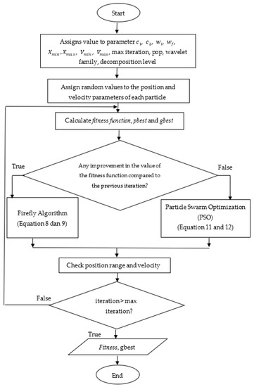
Figure 1.
Flowchart of wavelet family and decomposition level optimization using FAPSO algorithm.
3.4. Hierarchical Classification
In this study, the type of hierarchy structure employed is tree hierarchy, and the type of hierarchical classification used is Local Classification at the Parent Node (LCPN). Figure 2 illustrates an example of a three-level tree structure. In this hierarchy, there are five parent nodes: the root node, nodes 1, 2, 2.1, and 2.2. The nodes 1.1, 1.2, 2.1.1, 2.1.2, 2.2.1, and 2.2.2 make up a leaf or the last node on a branch. The exclusive sibling policy, which is explained in [73], is used to train the classification model. In Figure 2, for example, the shaded box denotes node 2.1, which is one of the parent nodes. Based on the exclusive sibling policy, node 2.1’s positive data set is node 2.1, while node 2.1’s negative data set is node 2.2.
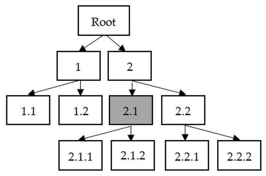
Figure 2.
Hierarchical classification using Local Classification on the Parent Node (LCPN).
The performance of the support vector machine (SVM) classifier is satisfactory when combined with the PseAAC feature representation approach [3]. The support vector machine (SVM) has been shown to be a robust classifier in multiple areas of biological analysis [66]. As a result, in this study, the SVM classifier is utilised in each parent node of the hierarchy. The training of each SVM model is done with a positive training dataset from the parent node and a negative training dataset from the parent’s sibling nodes.
The top-down hierarchical classification method is used to classify the test data for the classification phase. Referring to Figure 2, the classifier in the root node will classify the data to the node in the first level, which is class 1 or 2 only. This data will then be sent to the second level according to the classification results from the root node. For example, if the SVM classifier classifies new data into class 2, this data will be classified by the classifier into class 2.1 or 2.2. If the data is classified as node 2.1, the next classification is to the leaf nodes, which are nodes 2.1.1 or 2.1.2. This study used the binary SVM classifier and the ECOC model available in MATLAB R2019a software. The coding method used in this study is one-to-one classification (OVO), while the type of kernel used is Radial Basis Function (RBF).
3.5. Hierarchical Classification with Virtual Class
The top-down classification method has a weakness in which error propagation occurs. The error propagation problem is a classification error at the upper level of the hierarchy; this situation can continue up to the terminal node or leaf node [45,49,74,75]. This error can be reduced by the virtual class (VC) method. This virtual class method was introduced by [48] to overcome the problem of propagation errors in tree-type hierarchical classification. This method was also used in [49] to overcome error propagation in hierarchical text classification. It was found that the combination of the local hierarchical classification method on the parent node (LCPN) and the virtual class (VC) method successfully obtained high performance. The following is a description of the process to overcome the error propagation problem using the virtual class method.
In Figure 3, virtual nodes are built on the internal nodes of the hierarchy except the root node. V1, V2, V3, and V4 are virtual nodes. These nodes are connected to the parent node using a dashed line to indicate that this node does not belong to the child node of the parent node. For example, class 1 has training data from classes 1.1, 1.2, and a virtual class, V1. This virtual class V1 contains training data from class 1’s sibling nodes 2 and 3. Class 2 contains training data from classes 2.1, 2.2, and virtual class V2. This virtual class V2 contains training data from class 2’s sibling nodes 1 and 3.
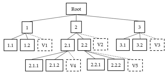
Figure 3.
Hierarchical classification using virtual classes.
The test data will be classified based on the top-down hierarchical classification method for the testing phase. If this test data is classified as a virtual class, this means that this test data is classified as the sibling node of the parent node. The classification of this test data will stop at that level.
3.6. Performance Evaluation
The proposed algorithm is evaluated using the five-fold cross-validation method whereby the data is divided into five subsets of relatively equal size. After training the SVM classifier with four subsets, its performance is evaluated with the fifth subset. This process is repeated five times to ensure that each subset is suitable for testing.
Four performance testing criteria-accuracy (A), precision (P), recall (R), and F-score (F)-have been used to measure how well the proposed techniques work (F). These measurement values are used to evaluate the classification performance of the developed method. Accuracy, precision, recall, and F-score values are defined in Equations (13)–(16), respectively. Equation (13) is used to find the accuracy value for each class in the hierarchy, where c(i) is the number of correctly classified protein sequences in class I and Total(i) is the total number of protein sequences in class i. In Equations (14)–(16), the values of true positive (TP), false negative (FN), true negative (TN), and false positive (FP) have been used. A true positive (TP) is when a positive case is correctly put into the positive class. A false negative (FN) is when a positive case is mistakenly put into the negative class. A true negative (TN) is a case that has been correctly labelled as negative, while a false positive (FP) is a case that has been labelled as positive even though it is negative.
4. Results
This paper proposes FAPSO as a feature extraction method and SVM as the hierarchical GPCR protein classification model. The proposed model is different from the traditional classification model as it is a combination of the following parts: (1) hybridization of the Firefly algorithm and Particle Swarm Optimization to select the suitable wavelet family and decomposition level and (2); a hierarchical classification strategy (LCPN with VC) to stop the incorrect classifications that occur with non-mandatory leaf node prediction (NMLNP) in internal hierarchy levels before reaching the leaf node. The results are analyzed according to three hierarchy levels: family, subfamily, and sub-subfamily. The family level consists of 5 classes; the subfamily level contains 38 classes; and the sub-subfamily level contains 87 classes.
The PseAAC features vector graph for one of the class A GPCR proteins is shown in Figure 4a. Using the Coiflet wavelet family 4 and 3 levels of decomposition, the DWT converted the PseAAC features into approximation coefficients and detail coefficients. The detailed wavelet coefficients for decomposition levels 1, 2, and 3 that contain local protein features are shown in Figure 4b–d. While Figure 4d shows the wavelet approximation coefficient with global features or rough characteristics of the protein. The number of global and local features produced depends on the number of decomposition levels. Decomposition level can be performed up to the log2 (N) level, where N is the length of the studied data. In this study, considering the size of the PseAAC feature used is 170, the maximum decomposition size allowed is seven levels. Here, we can see the advantage of the wavelet’s multiresolution analysis, which enables protein sequences to be studied using multiple decomposition levels.
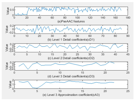
Figure 4.
Representation of PseAAC features for class A GPCR proteins using the Coiflet 4 DWT wavelet family with 3 decomposition level.
In this paper, the results are separated into two sections. The first section describes the chosen wavelet family and decomposition level, while the second section describes the algorithm’s performance.
4.1. Selection of Wavelet Family and Decomposition Level
Table 2 shows the wavelet families selected by the FAPSO algorithm for each of the five folds. Each fold of the data contained eleven wavelet families to represent the eleven nodes in the GPCR protein hierarchy, which are the root, family A, family B, family C, subfamily A Amine, subfamily A Hormone, subfamily A Nucleotide, subfamily A Peptide, subfamily A Thyro, subfamily Prostanoid, and subfamily C CalcSense. As a result, for the five folds of the data set, the total number of wavelet families is 55. The wavelet family and decomposition level selected by the FAPSO method were examined at eleven nodes of the hierarchy. Table 2 clearly shows that the wavelet family and decomposition level chosen at different nodes differ significantly. This supports the use of FAPSO, which determines the wavelet family and decomposition level at each class node automatically.
Table 2.
Selected wavelet family and decomposition level at each GPCR node.
Figure 5 shows how often each wavelet family is chosen at every level of the GPCR hierarchy. 15 GPCR proteins were chosen from the Biorthogonal family, 14 were chosen from the Reverse Biorthogonal family, 9 were chosen from the Daubechies family, 4 were chosen from the Symlet family, 5 were chosen from the Fejer–Korovkin family, 3 were chosen from the Dmeyer family, 3 were chosen from the Coiflet family, and 2 were chosen from the Haar family. Most protein classes are effectively represented by the Biorthogonal wavelet family since most scaling functions and wavelet functions in this family have a sudden change in shape. This fits with the rough shape and many sharp changes in the shape of PseAAC, as shown in Figure 4a. Furthermore, [76] mentioned that the Biorthogonal wavelet could get rid of redundant information from protein sequences, minimise feature information leakage and aliasing, let feature vectors represent the original sequence information, and improve prediction performance. FAPSO also selects the Daubechies and Fejer-Korovkin wavelets at least five times.
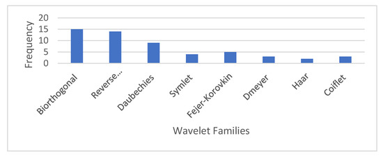
Figure 5.
Frequency of selection of each wavelet family at each node of the GPCR hierarchy.
Figure 6 depicts the frequency of decomposition levels to represent protein classes. In total, 15 of the 55 wavelet families used decomposition level 1, the highest level of decomposition used in feature representation. Decomposition level 1 yielded 85 approximation and 85 detail coefficients, accounting for half of the 170 PseAAC features. Decomposition level 1 preserved global and local information. Decomposition level 3 was used by 14 wavelet families. Decomposition level 2 was used by 11 wavelet families. Four wavelet families used level decomposition 4, six families used level decomposition 5, and four families used level decomposition 6. Decomposition level 7 was the fewest decomposition level chosen for the feature representation, with only one. A higher level of decomposition increases the number of detail coefficients while decreasing the number of approximation coefficients. This means that the protein class required more local information to represent it than global information.
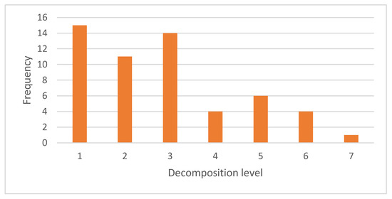
Figure 6.
Frequency of selection of each decomposition level at each node of the GPCR hierarchy.
4.2. GPCR Classification Performance without Virtual Class
Table 3 shows the performance for the classification of GPCR using SVM at the family level. It can be observed from the results shown that at the family level, FAPSO is the best feature extraction strategy. The performance level achieved by FAPSO was 97.9% for accuracy, precision, and recall. This illustrates that both PseAAC and FAPSO can be used to classify GPCRs at the family level with high accuracy.
Table 3.
GPCR classification performance for family level.
Table 4 shows the performance for the classification of GPCR using SVM at the subfamily level. As seen from the table, the results show that at the subfamily level, PseAAC is the best feature extraction strategy at this hierarchy level. The performance levels achieved by PseAAC were 85.3%, 87.7%, 87.7%, and 0.887% for accuracy, precision, recall and F-score, respectively. This indicates that PseAAC is good for characterizing the GPCR at the subfamily level. Nevertheless, the FAPSO algorithm achieved better precision than PseAAC at 88.9%. It means that FAPSO produced a lower false positive rate by using DWT features compared to PseAAC.
Table 4.
GPCR classification performance for subfamily level.
Table 5 displays the classification performance of GPCRs using SVM at the sub-subfamily level. This table demonstrates that at the sub-subfamily level, PseAAC has the highest accuracy, at 76.9%. While FAPSO has the highest precision, recall, and F-score values, which are 87.5%, 81.2%, and 84.4%, respectively.
Table 5.
GPCR classification performance for sub-subfamily level.
Table 4 and Table 5 demonstrate that the precision value for FAPSO classification results at the subfamily and sub-subfamily levels is greater than the accuracy value. This is indeed a good sign since high accuracy can also be attained by correctly identifying the dominating negative class. It has been shown that the GPCR protein has unbalanced data for each class [63,77]. Therefore, it is more crucial to obtain a high precision value [78]. In addition, the accuracy value is not a suitable statistic for data sets with imbalance [78]. The recall value was higher than the accuracy value, as seen in Table 5. This suggests that FAPSO worked effectively despite the imbalance that existed in the GPCR protein dataset.
From the observation, the performance of PseAAC and FAPSO decreased as the hierarchy level became deeper. This is because of the large number of classes (38 and 87, respectively) at the subfamily and sub-subfamily levels.
4.3. GPCR Classification Performance with Virtual Class
Table 6 shows the performance for the classification of GPCR using SVM with virtual class implementation at the subfamily level. First and foremost, the results are considerably different between PseAAC+VC and FAPSO+VC. FAPSO+VC gives better performance than PseAAC+VC. When comparing PseAAC against PseAAC+VC, the latter has higher accuracy, precision, recall and F-score values than the former, at 85.4%, 88.3%, 88.3%, and 0.833. As for FAPSO and FAPSO+VC, the FAPSO+VC also performs better than FAPSO. FAPSO+VC achieved 86.9% accuracy, 94.1% precision, 90.1% recall, and 0.921 F-score. At the subfamily level, it was found that false positive numbers had decreased for the FAPSO algorithm compared to the PseAAC algorithm after VC implementation. This is because these data have been classified at the VCs, which are in classes A, B, C, D, or E and therefore avoid the error propagation problem. There is also an increase in the true positive number of classes A and C, in which the data were classified accurately after VC implementation.
Table 6.
GPCR classification performance for subfamily level.
As for the performance at the sub-subfamily level shown in Table 7, when comparing PseAAC against PseAAC+VC, the latter has better accuracy, precision, recall and F-score values than the former, at 78.8%, 89.6%, 82.6%, and 0.86, respectively. As for FAPSO and FAPSO+VC, the FAPSO+VC also performs better than FAPSO. FAPSO+VC achieved 81.3% accuracy, 92.1% precision, 85.1% recall, and 0.844 F-score. At sub-subfamily level, false positive numbers have also decreased especially for sub-subfamily under subfamily A amine, A hormone, A Peptide and C CalcSense. It is found that the number of positive has increased especially for the subfamily A Amine, A Hormone and C CalcSense.
Table 7.
GPCR classification performance for sub-subfamily level.
It can be seen that virtual class consistently increased performance in all experiments, since it increases the likelihood of avoiding error propagation in the hierarchy by stopping the classification at an appropriate level.
Table 8 compares the GPCR protein classification accuracy performance obtained from this study and earlier research that made use of the same GDS data set. This study’s accuracy value at the family level was determined to be 97.9%, which is remarkably similar to the accuracy values in the studies of [57,61,63,64,66]. In this study, the second level of the hierarchy had an accuracy value of 86.9%. Nevertheless, [63] obtained higher accuracy values for the second level of the hierarchy, which is 89.2%. The accuracy percentage at the third level obtained by this study is 81.3%. Still, the research of [63], which received an accuracy value of 90.9%, produced the highest accuracy value for this third level.
Table 8.
Comparison of GPCR protein classification using the GDS dataset.
Although the accuracy of this study is lower than [63] at the subfamily and sub-subfamily level, their research focused on optimizing the GPCR protein classifiers. This study conversely attempted to optimize the representation of GPCR proteins at the feature level. Hence, compared to other studies, it was found that this study’s results are comparable to those by [56,57], which used the current trending deep learning method.
5. Discussion
In this study, the FAPSO feature representation method has helped identify the type of wavelet family and the appropriate decomposition level for each GPCR protein class representation. There are 82 wavelet families to select from, including the Daubechies, Coiflet, Meyer, Biorthogonal and Reverse Biorthogonal families. Each wavelet family has characteristics such as orthogonality, the number of vanishing moments, and the type of symmetry found in the scaling and wavelet functions. These features can be adjusted to the characteristics of the studied protein sequence. The convolution result between PseAAC features and the wavelet family will produce low-frequency or approximation and high-frequency or detail coefficients. The approximation coefficient contains coarse or global information about the studied protein sequence. Meanwhile, the detail coefficient contains important information found in the studied protein. In this study, the Biorthogonal wavelet is the most selected wavelet family representing GPCR protein classes by FAPSO. The Biorthogonal wavelet contained symmetric and compact support, which appears suitable to represent this protein.
The multiresolution analysis allows protein sequences to be studied using multiple decomposition levels and can be performed up to the log2 (N) level, where N is the length of the studied data. In this study, considering the size of the PseAAC feature used is 170, the maximum decomposition size allowed is seven levels. Different levels will produce many coefficients, which are global features and detail coefficients. FAPSO has identified that the root, family A, subfamily A Amine, and subfamily A Peptide nodes required decomposition level 1 to represent proteins in those classes. For family C and subfamily C CalcSense, decomposition levels 6 and 3 are required to represent proteins in that class. This is because protein C has a long and varied sequence size, in addition to a complex structure [54]. Therefore, the selection of the decomposition level also plays a vital role in determining the classification performance. This proves that each GPCR protein class requires a different wavelet family and decomposition level for feature representation.
Nevertheless, it can be concluded that the FAPSO optimization algorithm alone cannot improve the GPCR hierarchical protein classification performance compared to the PseAAC algorithm. In this study, the number of iterations used in the FAPSO optimization algorithm is 100 iterations on each parent node of the GPCR protein hierarchy. The classification performance may increase if the number of iterations increases or if the FAPSO parameters are changed to appropriate values.
The virtual class has been proposed to overcome the propagation error problem in top-down hierarchical classification. As a result, it can improve the classification results on the nodes in the hierarchy, especially when combined with the FAPSO feature representation algorithm.
6. Conclusions and Future Works
In this paper, we briefly studied the selection of optimized wavelet family and decomposition level by the FAPSO algorithm as the feature representation method and the virtual class method as the hierarchical classification method for GPCR protein. Based on the results, the most selected wavelet family and decomposition level chosen to represent GPCR classes by FAPSO were Biorthogonal wavelets and decomposition level 1. The choice of an adequate feature extraction strategy for protein classification is an important problem because they influence the performance measurement values according to the commonly used machine learning algorithm. It can be seen that virtual class consistently increases the performances in all experiments since it increases the likelihood of avoiding error propagation in the hierarchy by stopping the classification at an appropriate level.
This area of research still has a lot of space for growth and advancement. Data mining always runs into the imbalance data problem in the data set. A similar issue, with 60% of known GPCR protein sequences being proteins from the A family, also affects the GPCR dataset. To solve this issue, sampling techniques such as the Synthetic Minority Oversampling Technique (SMOTE) algorithm must be taken into account. SMOTE is an oversampling method that creates artificial samples from minority classes. After obtaining a synthetically balanced training set for each class, the classifier is trained.
Future work should investigate the best wavelet family and level of decomposition to represent the GPCR protein class. The trials carried out in this study used parameter values for the FAPSO algorithm based on prior work. The suitability of the parameters for FAPSO is not examined in this work. This necessitates a thorough investigation to establish the correct parameter values needed for the FAPSO algorithm as an algorithm for choosing the wavelet family and decomposition level.
There are various implementation strategies for hierarchical classification. This includes global hierarchical classification, which does not have the same issue with errors propagating as in the present study. A training set for global classification is used to create a sophisticated classification model. When classifying, this takes into account the entire class structure. Each test data set will be categorised using the test phase’s classification model. This global hierarchical classification method is expected to enhance the performance of the hierarchical classification of GPCR proteins.
Author Contributions
Conceptualization, N.A.M.K.; methodology, N.A.M.K.; software, N.A.M.K.; validation, N.A.M.K., A.A.B. and S.Z.; formal analysis, N.A.M.K. and A.A.B.; investigation, N.A.M.K. and A.A.B.; resources, N.A.M.K.; writing—original draft preparation, N.A.M.K.; writing—review and editing, N.A.M.K., A.A.B. and S.Z.; visualization, N.A.M.K.; supervision, A.A.B. and S.Z.; project administration, A.A.B. and S.Z.; funding acquisition, A.A.B. and S.Z. All authors have read and agreed to the published version of the manuscript.
Funding
This study was financially supported by the Malaysia Ministry of Higher Education (MOHE) and Universiti Kebangsaan Malaysia-TAP-K012964, GUP-2020-089.
Institutional Review Board Statement
Not applicable.
Informed Consent Statement
Not applicable.
Data Availability Statement
Data supporting the proposed approaches in this study were collected from https://www.cs.kent.ac.uk/projects/biasprofs/downloads.html (accessed on 23 March 2014).
Conflicts of Interest
The authors declare no conflict of interest.
Abbreviations
The following abbreviations are used in this manuscript:
| WT | Wavelet Transform |
| DWT | Discrete Wavelet Transform |
| SVM | Support Vector Machine |
| PSO | Particle Swarm Optimization |
| FA | Firefly Algorithm |
| FAPSO | Firefly Algorithm-Particle Swarm Optimization |
| VC | Virtual Class |
| DB | Daubechies |
| Coif | Coiflet |
| Sym | Symlet |
| Dmey | Discrete Meyer |
| FK | Fejer–Korovkin |
| Bior | Biorthogonal |
| RBior | Reverse Biorthogonal |
| GPCR | G-Protein Coupled Receptor |
| PseAAC | Pseudo Amino Acid Composition |
| LCPN | Local Classification at the Parent Node |
| NMLNP | Non-Mandatory Leaf Node Prediction |
References
- Naik, A. Hierarchical Classsification with Rare Categories and Inconsistencies. Ph.D. Thesis, George Mason University, Fairfax, VA, USA, 2017. [Google Scholar]
- Secker, A.; Davies, M.N.; Freitas, A.A.; Clark, E.; Timmis, J.; Flower, D.R. Hierarchical Classification of G-Protein-Coupled Receptors with Data-Driven Selection of Attributes and Classifiers. Int. J. Data Min. Bioinform. 2010, 4, 191–210. [Google Scholar] [CrossRef] [PubMed]
- Bekhouche, S.; Ben Ali, Y.M. Optimizing the Identification of GPCR Function. In Proceedings of the New Challenges in Data Sciences, Kenitra, Morocco, 28–29 March 2019; pp. 1–5. [Google Scholar] [CrossRef]
- Wang, T.; Li, L.; Huang, Y.A.; Zhang, H.; Ma, Y.; Zhou, X. Prediction of Protein-Protein Interactions from Amino Acid Sequences Based on Continuous and Discrete Wavelet Transform Features. Molecules 2018, 23, 823. [Google Scholar] [CrossRef] [PubMed]
- Chou, K.-C. Pseudo Amino Acid Composition and Its Applications in Bioinformatics, Proteomics and System Biology. Curr. Proteom. 2009, 6, 262–274. [Google Scholar] [CrossRef]
- Ru, X.; Wang, L.; Li, L.; Ding, H.; Ye, X.; Zou, Q. Exploration of the Correlation between GPCRs and Drugs Based on a Learning to Rank Algorithm. Comput. Biol. Med. 2020, 119, 103660. [Google Scholar] [CrossRef]
- Ao, C.; Gao, L.; Yu, L. Identifying G-Protein Coupled Receptors Using Mixed-Feature Extraction Methods and Machine Learning Methods. IEEE Access 2020. early access. [Google Scholar] [CrossRef]
- Zhao, Z.Y.; Huang, W.Z.; Zhan, X.K.; Pan, J.; Huang, Y.A.; Zhang, S.W.; Yu, C.Q. An Ensemble Learning-Based Method for Inferring Drug-Target Interactions Combining Protein Sequences and Drug Fingerprints. Biomed Res. Int. 2021, 2021, 9933873. [Google Scholar] [CrossRef]
- Li, Y.; Huang, Y.A.; You, Z.H.; Li, L.P.; Wang, Z. Drug-Target Interaction Prediction Based on Drug Fingerprint Information and Protein Sequence. Molecules 2019, 24, 2999. [Google Scholar] [CrossRef]
- Davies, M.N.; Secker, A.; Freitas, A.A.; Mendao, M.; Timmis, J.; Flower, D.R. On the Hierarchical Classification of G Protein-Coupled Receptors. Bioinformatics 2007, 23, 3113–3118. [Google Scholar] [CrossRef]
- Yu, B.; Li, S.; Qiu, W.Y.; Chen, C.; Chen, R.X.; Wang, L.; Wang, M.H.; Zhang, Y. Accurate Prediction of Subcellular Location of Apoptosis Proteins Combining Chou’s PseAAC and PsePSSM Based on Wavelet Denoising. Oncotarget 2017, 8, 107640–107665. [Google Scholar] [CrossRef]
- Najeeb, S.; Raj, N. Wavelet Analysis in Current Cancer Genome to Identify Driver Mutation. Int. J. Eng. Res. Technol. 2017, 5, 1–7. [Google Scholar]
- Meng, T.; Soliman, A.T.; Shyu, M.L.; Yang, Y.; Chen, S.C.; Iyengar, S.S.; Yordy, J.S.; Iyengar, P. Wavelet Analysis in Current Cancer Genome Research: A Survey. IEEE/ACM Trans. Comput. Biol. Bioinforma. 2013, 10, 1442–1459. [Google Scholar] [CrossRef]
- Kulkarni, O.C.; Vigneshwar, R.; Jayaraman, V.K.; Kulkarni, B.D. Identification of Coding and Non-Coding Sequences Using Local Hölder Exponent Formalism. Bioinformatics 2005, 21, 3818–3823. [Google Scholar] [CrossRef]
- Chen, B.; Li, Y.; Zeng, N. Centralized Wavelet Multiresolution for Exact Translation Invariant Processing of ECG Signals. IEEE Access 2019, 7, 42322–42330. [Google Scholar] [CrossRef]
- Saini, S.; Dewan, L. Performance Comparison of First Generation and Second Generation Wavelets in the Perspective of Genomic Sequence Analysis. Int. J. Pure Appl. Math. 2018, 118, 417–442. [Google Scholar]
- Gayathri, T.T.; Christe, S.A. Wavelet Analysis in Prediction and Identification of Cancerous Genes. Int. J. Sci. Eng. Res. 2017, 8, 720–727. [Google Scholar]
- Hou, W.; Pan, Q.; Peng, Q.; He, M. A New Method to Analyze Protein Sequence Similarity Using Dynamic Time Warping. Genom. J. 2017, 109, 123–130. [Google Scholar] [CrossRef]
- Qiu, J.-D.; Sun, X.-Y.; Huang, J.-H.; Liang, R.-P. Prediction of the Types of Membrane Proteins Based on Discrete Wavelet Transform and Support Vector Machines. Protein J. 2010, 29, 114–119. [Google Scholar] [CrossRef]
- Elbir, A.; Ilhan, H.O.; Serbes, G.; Aydin, N. Short Time Fourier Transform Based Music Genre Classification. In Proceedings of the 2018 Electric Electronics, Computer Science, Biomedical Engineerings' Meeting (EBBT), Istanbul, Turkey, 8–19 April 2018; pp. 1–4. [Google Scholar] [CrossRef]
- Aggarwal, C.C. On Effective Classification of Strings with Wavelets. In Proceedings of the Eighth ACM SIGKDD International Conference on Knowledge Discovery and Data Mining, Edmonton, AB, Canada, 23–26 July 2002; pp. 163–172. [Google Scholar] [CrossRef]
- Mai, T.D.; Ngo, T.D.; Le, D.D.; Duong, D.A.; Hoang, K.; Satoh, S. Using Node Relationships for Hierarchical Classification. In Proceedings of the 2016 IEEE International Conference on Image Processing (ICIP), Phoenix, AZ, USA, 25–28 September 2016; Volume 2016, pp. 514–518. [Google Scholar] [CrossRef]
- De Trad, C.; Fang, Q.; Cosic, I. An Overview of Protein Sequence Comparisons Using Wavelets. In Proceedings of the IEEE Engineering in Medicine and Biology Society, Istanbul, Turkey, 25–28 October 2001; pp. 115–119. [Google Scholar]
- Liò, P. Wavelets in Bioinformatics and Computational Biology: State of Art and Perspectives. Bioinformatics 2003, 19, 2–9. [Google Scholar] [CrossRef]
- Haimovich, A.D.; Byrne, B.; Ramaswamy, R.; Welsh, W.J. Wavelet Analysis of DNA Walks. J. Comput. Biol. 2006, 13, 1289–1298. [Google Scholar] [CrossRef]
- Germán-Salló, Z.; Strnad, G. Signal Processing Methods in Fault Detection in Manufacturing Systems. Procedia Manuf. 2018, 22, 613–620. [Google Scholar] [CrossRef]
- Alyasseri, Z.A.A.; Khader, A.T.; Al-Betar, M.A.; Abasi, A.K.; Makhadmeh, S.N. EEG Signals Denoising Using Optimal Wavelet Transform Hybridized with Efficient Metaheuristic Methods. IEEE Access 2020, 8, 10584–10605. [Google Scholar] [CrossRef]
- Aprillia, H.; Yang, H.T.; Huang, C.M. Optimal Decomposition and Reconstruction of Discrete Wavelet Transformation for Short-Term Load Forecasting. Energies 2019, 12, 4654. [Google Scholar] [CrossRef]
- Semnani, A.; Wang, L.; Ostadhassan, M.; Nabi-Bidhendi, M.; Araabi, B.N. Time-Frequency Decomposition of Seismic Signals via Quantum Swarm Evolutionary Matching Pursuit. Geophys. Prospect. 2019, 67, 1701–1719. [Google Scholar] [CrossRef]
- Jang, Y.I.; Sim, J.Y.; Yang, J.R.; Kwon, N.K. The Optimal Selection of Mother Wavelet Function and Decomposition Level for Denoising of Dcg Signal. Sensors 2021, 21, 1851. [Google Scholar] [CrossRef]
- He, H.; Tan, Y.; Wang, Y. Optimal Base Wavelet Selection for ECG Noise Reduction Using a Comprehensive Entropy Criterion. Entropy 2015, 17, 6093–6109. [Google Scholar] [CrossRef]
- Ngui, W.K.; Leong, M.S.; Hee, L.M.; Abdelrhman, A.M. Wavelet Analysis: Mother Wavelet Selection Methods. Appl. Mech. Mater. 2013, 393, 953–958. [Google Scholar] [CrossRef]
- Rhif, M.; Abbes, A.B.; Farah, I.R.; Martínez, B.; Sang, Y. Wavelet Transform Application for/in Non-Stationary Time-Series Analysis: A Review. Appl. Sci. 2019, 9, 1345. [Google Scholar] [CrossRef]
- Guarnizo, C.; Orozco, A.A.; Alvarez, M. Optimal Sampling Frequency in Wavelet-Based Signal Feature Extraction Using Particle Swarm Optimization. In Proceedings of the 35th Annual International Conference of the IEEE Engineering in Medicine and Biology Society, Osaka, Japan, 3–7 July 2013; Volume 2013, pp. 993–996. [Google Scholar] [CrossRef]
- Caramia, C.; De Marchis, C.; Schmid, M. Optimizing the Scale of a Wavelet-Based Method for the Detection of Gait Events from a Waist-Mounted Accelerometer under Different Walking Speeds. Sensors 2019, 19, 1869. [Google Scholar] [CrossRef]
- Zhang, Z.; Telesford, Q.K.; Giusti, C.; Lim, K.O.; Bassett, D.S. Choosing Wavelet Methods, Filters, and Lengths for Functional Brain Network Construction. PLoS ONE 2016, 11, e0157243. [Google Scholar] [CrossRef]
- Chen, D.; Wan, S.; Xiang, J.; Bao, F.S. A High-Performance Seizure Detection Algorithm Based on Discrete Wavelet Transform (DWT) and EEG. PLoS ONE 2017, 12, e0173138. [Google Scholar] [CrossRef]
- Oltean, G.; Ivanciu, L.N. Computational Intelligence and Wavelet Transform Based Metamodel for Efficient Generation of Not-yet Simulated Waveforms. PLoS ONE 2016, 11, e0146602. [Google Scholar] [CrossRef] [PubMed]
- Tao, H.; Zain, J.M.; Ahmed, M.M.; Abdalla, A.N.; Jing, W. A Wavelet-Based Particle Swarm Optimization Algorithm for Digital Image Watermarking. Integr. Comput. Aided. Eng. 2012, 19, 81–91. [Google Scholar] [CrossRef]
- Abdullah, N.A.; Rahim, N.A.; Gan, C.K.; Adzman, N.N. Forecasting Solar Power Using Hybrid Firefly and Particle Swarm Optimization (HFPSO) for Optimizing the Parameters in a Wavelet Transform-Adaptive Neuro Fuzzy Inference System (WT-ANFIS). Appl. Sci. 2019, 9, 3214. [Google Scholar] [CrossRef]
- Ngo, T.T.; Sadollah, A.; Kim, J.H. A Cooperative Particle Swarm Optimizer with Stochastic Movements for Computationally Expensive Numerical Optimization Problems. J. Comput. Sci. 2016, 13, 68–82. [Google Scholar] [CrossRef]
- Kora, P.; Rama Krishna, K.S. Hybrid Firefly and Particle Swarm Optimization Algorithm for the Detection of Bundle Branch Block. Int. J. Cardiovasc. Acad. 2016, 2, 44–48. [Google Scholar] [CrossRef]
- Aydilek, İ.B. A Hybrid Firefly and Particle Swarm Optimization Algorithm for Computationally Expensive Numerical Problems. Appl. Soft Comput. J. 2018, 66, 232–249. [Google Scholar] [CrossRef]
- Zhang, L.; Shah, S.K.; Kakadiaris, I.A. Hierarchical Multi-Label Classification Using Fully Associative Ensemble Learning. Pattern Recognit. 2017, 70, 89–103. [Google Scholar] [CrossRef]
- Zhu, S.; Wei, X.Y.; Ngo, C.W. Collaborative Error Reduction for Hierarchical Classification. Comput. Vis. Image Underst. 2014, 124, 79–90. [Google Scholar] [CrossRef]
- Nakano, F.K.; Pinto, W.J.; Pappa, G.L.; Cerri, R. Top-down Strategies for Hierarchical Classification of Transposable Elements with Neural Networks. In Proceedings of the 2017 International Joint Conference on Neural Networks, Anchorage, AK, USA, 14–19 May 2017; Volume 2017, pp. 2539–2546. [Google Scholar] [CrossRef]
- Ramírez-Corona, M.; Sucar, L.E.; Morales, E.F. Hierarchical Multilabel Classification Based on Path Evaluation. Int. J. Approx. Reason. 2016, 68, 179–193. [Google Scholar] [CrossRef]
- Ying, C.; Run Ying, D. Novel Top-down Methods for Hierarchical Text Classification. Procedia Eng. 2011, 24, 329–334. [Google Scholar] [CrossRef][Green Version]
- Stein, R.A.; Jaques, P.A.; Valiati, J.F. An Analysis of Hierarchical Text Classification Using Word Embeddings. Inf. Sci. 2019, 471, 216–232. [Google Scholar] [CrossRef]
- Alhosaini, K.; Azhar, A.; Alonazi, A.; Al-Zoghaibi, F. GPCRs: The Most Promiscuous Druggable Receptor of the Mankind. Saudi Pharm. J. 2021, 29, 539–551. [Google Scholar] [CrossRef] [PubMed]
- Li, M.; Ling, C.; Gao, J. An Efficient CNN-Based Classification on G-Protein Coupled Receptors Using TF-IDF and N-Gram. In Proceedings of the 2017 IEEE Symposium on Computers and Communications (ISCC), Heraklion, Greece, 3–6 July 2017; pp. 924–931. [Google Scholar]
- Davies, M.; Secker, A.; Freitas, A. Optimizing Amino Acid Groupings for GPCR Classification. Bioinformatics 2008, 24, 1980–1986. [Google Scholar] [CrossRef] [PubMed]
- Karchin, R.; Karplus, K.; Haussler, D. Classifying G-Protein Coupled Receptors with Support Vector Machines. Bioinformatics 2002, 18, 147–159. [Google Scholar] [CrossRef]
- Cruz-Barbosa, R.; Ramos-Pérez, E.G.; Giraldo, J. Representation Learning for Class C G Protein-Coupled Receptors Classification. Molecules 2018, 23, 690. [Google Scholar] [CrossRef]
- Li, M.; Ling, C.; Xu, Q.; Gao, J. Classification of G-Protein Coupled Receptors Based on a Rich Generation of Convolutional Neural Network, N-Gram Transformation and Multiple Sequence Alignments. Amino Acids 2018, 50, 255–266. [Google Scholar] [CrossRef]
- Paki, R.; Nourani, E.; Farajzadeh, D. Classification of G Protein-Coupled Receptors Using Attention Mechanism. Gene Rep. 2020, 21, 100882. [Google Scholar] [CrossRef]
- Seo, S.; Oh, M.; Park, Y.; Kim, S. DeepFam: Deep Learning Based Alignment-Free Method for Protein Family Modeling and Prediction. Bioinformatics 2018, 34, i254–i262. [Google Scholar] [CrossRef]
- Qiu, J.-D.; Huang, J.-H.; Liang, R.-P.; Lu, X.-Q. Prediction of G-Protein-Coupled Receptor Classes Based on the Concept of Chou’s Pseudo Amino Acid Composition: An Approach from Discrete Wavelet Transform. Anal. Biochem. 2009, 390, 68–73. [Google Scholar] [CrossRef]
- Guo, Y.Z.; Li, M.; Lu, M.; Wen, Z.; Wang, K.; Li, G.; Wu, J. Classifying G Protein-Coupled Receptors and Nuclear Receptors on the Basis of Protein Power Spectrum from Fast Fourier Transform. Amino Acids 2006, 30, 397–402. [Google Scholar] [CrossRef]
- Tiwari, A.K. Prediction of G-Protein Coupled Receptors and Their Subfamilies by Incorporating Various Sequence Features into Chou’s General PseAAC. Comput. Methods Programs Biomed. 2016, 134, 197–213. [Google Scholar] [CrossRef] [PubMed]
- Naveed, M.; Khan, A.U. GPCR-MPredictor: Multi-Level Prediction of G Protein-Coupled Receptors Using Genetic Ensemble. Amino Acids 2012, 42, 1809–1823. [Google Scholar] [CrossRef] [PubMed]
- Zia-ur-Rehman, B.S.P.; Khan, A. Identifying GPCRs and Their Types with Chou’s Pseudo Amino Acid Composition: An Approach from Multi-Scale Energy Representation and Position Specific Scoring Matrix. Protein Pept. Lett. 2012, 19, 890–903. [Google Scholar] [CrossRef] [PubMed]
- Zekri, M.; Alem, K.; Souici-Meslati, L. Immunological Computation for Protein Function Prediction. Fundam. Inform. 2015, 139, 91–114. [Google Scholar] [CrossRef]
- Rehman, Z.-U.; Mirza, M.T.; Khan, A.; Xhaard, H. Predicting G-Protein-Coupled Receptors Families Using Different Physiochemical Properties and Pseudo Amino Acid Composition. Methods Enzymol. 2013, 522, 61–79. [Google Scholar] [CrossRef]
- Secker, A.; Davies, M.N.; Freitas, A.A.; Timmis, J.; Clark, E.; Flower, D.R. An Artificial Immune System for Clustering Amino Acids in the Context of Protein Function Classification. J. Math. Model. Algorithms 2009, 8, 103–123. [Google Scholar] [CrossRef]
- Gao, Q.B.; Ye, X.F.; He, J. Classifying G-Protein-Coupled Receptors to the Finest Subtype Level. Biochem. Biophys. Res. Commun. 2013, 439, 303–308. [Google Scholar] [CrossRef]
- Shen, H.B.; Chou, K.C. PseAAC: A Flexible Web Server for Generating Various Kinds of Protein Pseudo Amino Acid Composition. Anal. Biochem. 2008, 373, 386–388. [Google Scholar] [CrossRef]
- Dao, F.Y.; Yang, H.; Su, Z.D.; Yang, W.; Wu, Y.; Ding, H.; Chen, W.; Tang, H.; Lin, H. Recent Advances in Conotoxin Classification by Using Machine Learning Methods. Molecules 2017, 22, 1057. [Google Scholar] [CrossRef]
- Shaker, A. Comparison Between Orthogonal and Bi-Orthogonal Wavelets. J. Southwest Jiatong Univ. 2020, 55, 2. [Google Scholar] [CrossRef]
- Ahuja, N.; Lertrattanapanich, L.; Bose, N.K. Properties Determining Choice of Mother Wavelet. IEE Proc. Vis. Image Signal Process. 2005, 152, 205–212. [Google Scholar] [CrossRef]
- Dogra, A.; Goyal, B.; Agrawal, S. Performance Comparison of Different Wavelet Families Based on Bone Vessel Fusion. Asian J. Pharm. 2016, 2016, 9–12. [Google Scholar]
- Yu, B.; Lou, L.; Li, S.; Zhang, Y.; Qiu, W.; Wu, X.; Wang, M.; Tian, B. Prediction of Protein Structural Class for Low-Similarity Sequences Using Chou’s Pseudo Amino Acid Composition and Wavelet Denoising. J. Mol. Graph. Model. 2017, 76, 260–273. [Google Scholar] [CrossRef] [PubMed]
- Silla, C.N., Jr.; Freitas, A. A Survey of Hierarchical Classification across Different Application Domains. Data Min. Knowl. Discov. 2010, 22, 31–72. [Google Scholar] [CrossRef]
- Shen, W.; Wei, Z.; Li, Q.; Zhang, H.; Duoqian, M. Three-Way Decisions Based Blocking Reduction Models in Hierarchical Classification. Inf. Sci. 2020, 523, 63–76. [Google Scholar] [CrossRef]
- Liu, Y.; Dou, Y.; Jin, R.; Li, R.; Qiao, P. Hierarchical Learning with Backtracking Algorithm Based on the Visual Confusion Label Tree for Large-Scale Image Classification. Vis. Comput. 2021, 98, 897–917. [Google Scholar] [CrossRef]
- Yu, B.; Li, S.; Chen, C.; Xu, J.; Qiu, W.; Wu, X.; Chen, R. Prediction Subcellular Localization of Gram-Negative Bacterial Proteins by Support Vector Machine Using Wavelet Denoising and Chou’s Pseudo Amino Acid Composition. Chemom. Intell. Lab. Syst. 2017, 167, 102–112. [Google Scholar] [CrossRef]
- Gu, Q.; Ding, Y.-S.; Zhang, T.-L. Prediction of G-Protein-Coupled Receptor Classes in Low Homology Using Chous Pseudo Amino Acid Composition with Approximate Entropy and Hydrophobicity Patterns. Protein Pept. Lett. 2010, 17, 559–567. [Google Scholar] [CrossRef]
- Juba, B.; Le, H.S. Precision-Recall versus Accuracy and the Role of Large Data Sets. In Proceedings of the AAAI Conference on Artificial Intelligence, Honolulu, Hawaii, USA, 27 January–1 February 2019; Volume 33, pp. 4039–4048. [Google Scholar] [CrossRef]
- Secker, A.; Davies, M.N.; Freitas, A.A.; Timmis, J.; Mendao, M.; Flower, D.R. An Experimental Comparison of Classification Algorithms for the Hierarchical Prediction of Protein Function Classification of GPCRs. Mag. Br. Comput. Soc. Spec. Group AI 2007, 9, 17–22. [Google Scholar]
Publisher’s Note: MDPI stays neutral with regard to jurisdictional claims in published maps and institutional affiliations. |
© 2022 by the authors. Licensee MDPI, Basel, Switzerland. This article is an open access article distributed under the terms and conditions of the Creative Commons Attribution (CC BY) license (https://creativecommons.org/licenses/by/4.0/).