Analysis of Chemical Components of Fine Particulate Matter Observed at Fukuoka, Japan, in Spring 2020 and Their Transport Paths

Abstract

Focusing on the components of fine particulate matter, i.e., PM_2.5, we have analyzed the factors that led to the high concentrations of each chemical component in PM_2.5 during our observations in Fukuoka, Japan in spring 2020. The backward trajectory showed that air masses reached Fukuoka via the Yellow Sea and the southern part of South Korea when PM_2.5 and each chemical component were high in concentrations. On the other hand, diurnal variations in ozone were also observed, suggesting that both transboundary and local air pollution are involved. Air masses reached the southern part of the Kyushu region when only sulfate concentrations were high. A volcano eruption led the high sulfate concentration. When only polycyclic aromatic hydrocarbons (PAHs) concentrations were high, air masses often reached the northern part of Kyushu, indicating that there may be a specific local source for PAHs.

1. Introduction

The achievement rate of the Environmental Quality Standards (EQSs) for concentrations of fine particulate matter (PM_2.5) in Japan has increased year by year, with more than 98% of stations achieving EQSs in 2019 [1]. According to a report by the Ministry of the Environment, Japan, the number of effective monitoring stations for PM_2.5 in Japan in 2019 was 1073 (835 stations in residential areas and 238 road-side stations). The number of monitoring stations that achieved the environmental standard (achievement rate) was 824 (98.7%) for stations in residential areas and 234 (98.3%) for road-side stations [1]. However, both long-term and short-term EQSs for PM_2.5 have not been achieved in northern Kyushu and several locations in the Seto Inland Sea. This suggests that there is an impact of transboundary air pollution from the Asian continent in the northern Kyushu area and other areas in addition to the impact of domestic sources. Fukuoka and the northern Kyushu area is located in the west of Japan and is affected by transboundary air pollution from the Asian continent from winter to spring [2,3,4,5,6,7,8,9].

Michikawa et al. [10] reported that a 10 μgm⁻³ increase in PM_2.5 results in an approximately 1.3% increase in deaths in Japan. Kojima et al. [11] also reported that fine particulate matter exposure relates to out-of-hospital cardiac arrest. There is a lot of evidence for PM_2.5 causing adverse effects on human health [12]. It is well known that particulate matter (PM) contains a variety of substances, including ions such as sulfate and nitrate, metals such as copper and iron, black carbon (elemental carbon), organic carbon and polycyclic aromatic hydrocarbons (PAHs) formed from organic compounds. It is not yet sufficiently known which substances affect health, though there appear to be several reports which mentioned the link between chemical components and their health effects [13,14]. Since human health is considered to be affected when concentrations of PM and each component are high, it is considered important to elucidate the factors that contribute to high concentrations of PM components.

We conducted a comprehensive project to elucidate the effects of PM_2.5 and PAHs contained in the particles on respiratory diseases. We collected airborne particles in Fukuoka and measured the chemical composition of the PM_2.5 particles. Our epidemiological analysis team is investigating the association between chemical components and respiratory diseases. As part of this project, the analysis of PAHs was reported by Pham et al. [15].

In this study, we focus on the chemical components of PM_2.5, aiming to clarify whether they show the same behavior in the atmosphere. We report the results of our analysis of the factors that led to the high concentrations of each chemical component in PM_2.5 observed in Fukuoka during the spring of 2020.

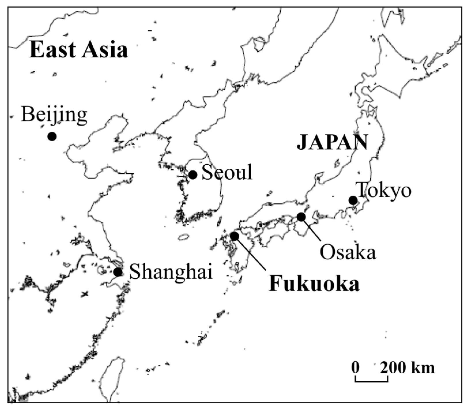
2. Materials and Methods

The location of Fukuoka is shown in Figure 1. Fukuoka is a large city with a population of 1.5 million. It is located in the west of Japan and is subject to transboundary air pollution during the winter and spring seasons [5,6,7,8,9,15].

The observation period was from February to April 2020. PM was collected by a high-volume air sampler (HV-RW, Sibata Scientific Technology Ltd., Tokyo, Japan) with a slit-type PM_2.5 separator installed on the roof of the National Hospital Organization Fukuoka National Hospital (Minami-ku, Fukuoka, Japan) at a flow rate of 1000 L/min on a fluoroplastic binder glass fiber filter (TX40HI20WW, Pall Corporation, Port Washington, WI, USA) for approximately 24 h. The filter that collected PM_2.5 was cut for PAHs and ion analysis. PAHs were analyzed by Kanazawa University [15,16,17], and The National Institute for Environmental Studies analyzed ionic components. Filters were soaked in ultrapure water, irradiated with ultrasonic waves, filtered through disk filters (pore size 0.45 µm), and the ionic components were analyzed by ion chromatography (Prominence, Shimadzu Corporation, Kyoto, Japan). Ions analyzed were sulfate, nitrate, chloride, sodium, ammonium, magnesium, calcium, and potassium ions.

For PM_2.5 mass concentration, trace metals including metalloids (Ti, V, Cr, Mn, Fe, Ni, Cu, Zn, As, Pb, Al, Si, S, K, and Ca), elemental carbon (EC), and organic carbon (OC) were measured at City Hall (Chuo-ku, Fukuoka, Japan, for PM_2.5), Fukuoka University (Jonan-ku, Fukuoka, Japan, for metals, EC, and OC); we used data measured by the Ministry of the Environment, Japan, which are publicly available [18]. Daily averages of trace metals and OC/EC data with 4 h and 1 h time resolutions were calculated. Ozone was measured by ourselves at Fukuoka University by using ultraviolet absorption spectrometry in accordance with the ozone standard measurement method established by the Japanese Ministry of the Environment (Model 49i, Thermo Fisher Scientific Inc., Waltham, MA, USA). Ozone was measured with a time resolution of 1 min and daily averages were also calculated. For meteorological data (temperature, relative humidity, solar radiation, wind speed and wind direction), we used data from the Fukuoka Meteorological Observatory, which is publicly available [19]. The NOAA’s HYSPLIT (The Hybrid Single-Particle Lagrangian Integrated Trajectory model) system was used to estimate air mass transport pathways [20,21].

3. Results and Discussion

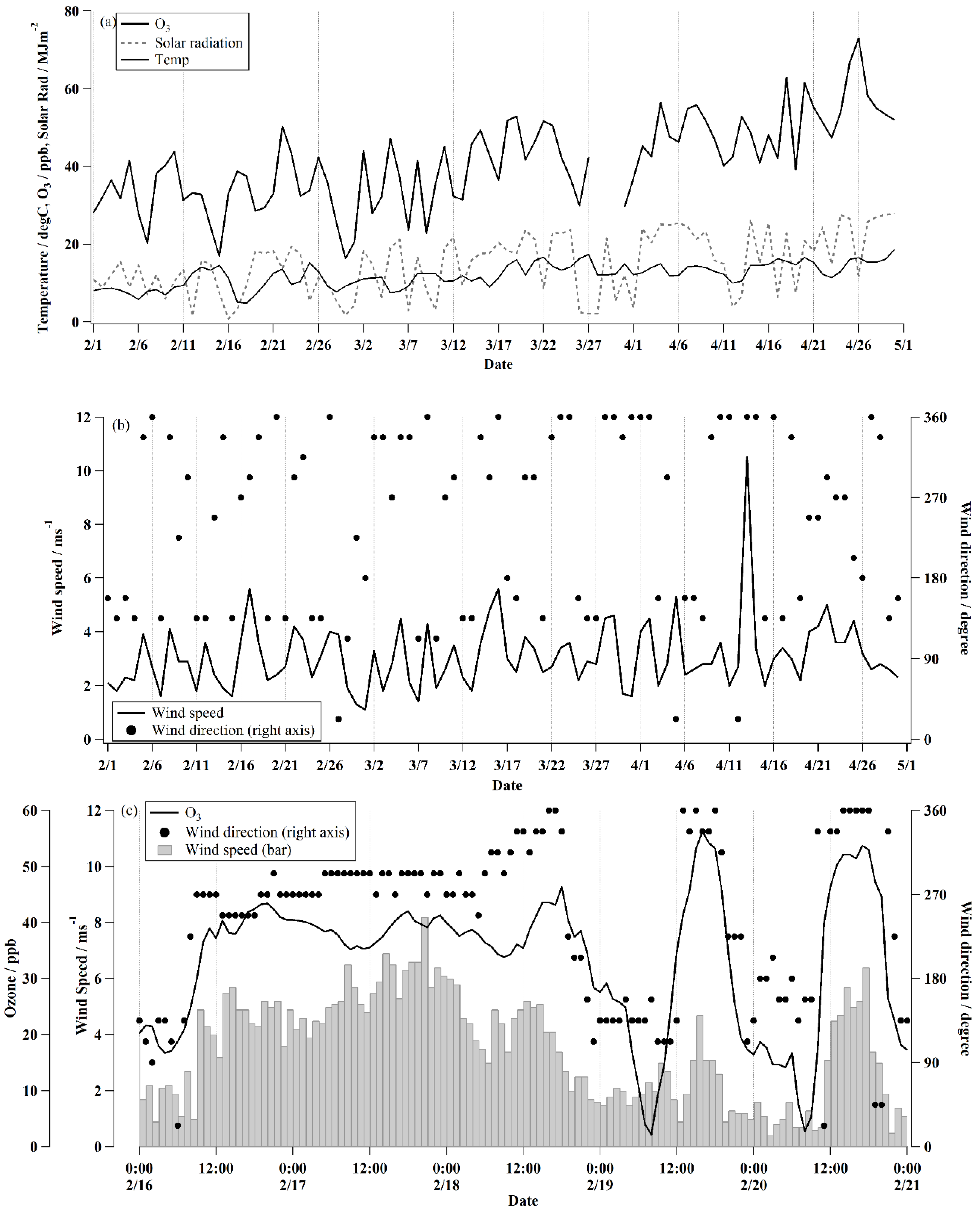
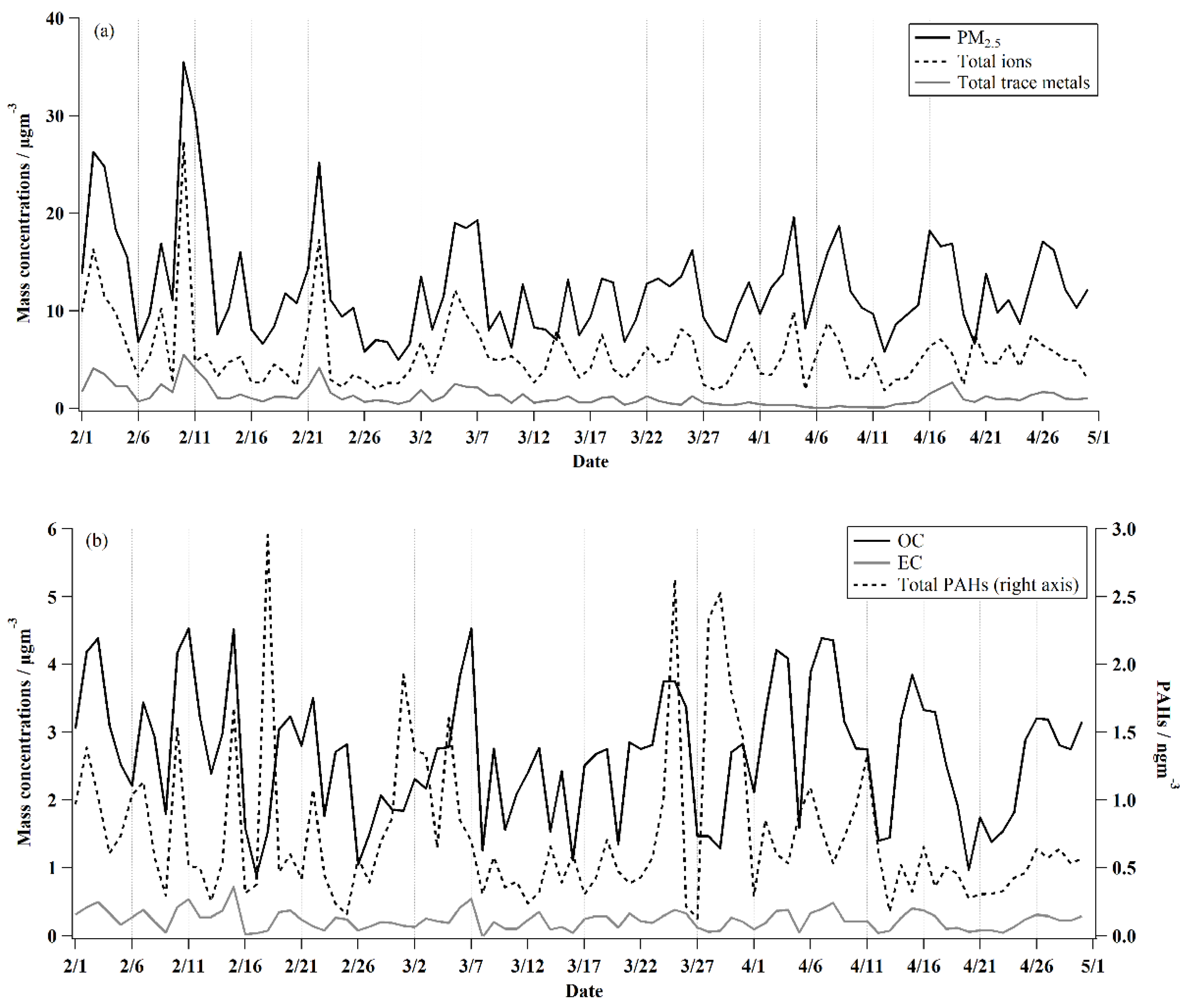
3.1. Overview of Results from February to April in 2020

The results for ozone and meteorological data for February–April in 2020 are shown in Figure 2. The ozone and solar radiation data in Figure 2a shows a gradual seasonal progression from February to April. As solar radiation increase, ozone concentration (mole mixing ratio) also increases. In particular, ozone concentration exceeded the EQSs of oxidant, which is 60 ppb, on some days in the latter half of April, presumably because photochemical reactions became more active with the increase in solar radiation in spring. Figure 2b shows the wind speed and direction. Due to the topography of the Fukuoka area, northwesterly sea breezes prevail during the daytime and southeasterly land breezes prevail during the nighttime [22,23]. The results from the Fukuoka Meteorological Observatory are daily averages and do not show sea and land breezes clearly during the day and night, but they do indicate that winds from the west-north, and southeast are dominant as the main wind directions. We plot hourly data of ozone, wind speed and wind direction data in Figure 2c. From the afternoon of 16 to the afternoon of 18 February, northerly winds were dominant, with wind speeds stronger than 3 ms⁻¹. At the same period, ozone concentration, especially at night, hardly dropped and showed no diurnal variations. In this case, we think that transboundary air pollution is dominant [9]. On the other hand, from 19 to 20 February, the ozone showed diurnal variations with southeasterly winds in the morning and evening and northerly winds in the afternoon, showing typical sea-land breeze in Fukuoka, as mentioned above. In this case, we think that local influence is relatively strong [9,22,23]. Thus, it is useful to refer to the diurnal variation data of ozone and wind direction when examining the influence of either transboundary air pollution or local pollution.

Note that the daily average of ozone is about 33–39 ppb from 16 to 18 February, but less than 30 ppb on 19 and 20 February. On average, the ozone concentration tends to be relatively higher when transboundary air pollution continues [9].

Figure 3 shows the results of concentrations of PM_2.5 and major chemical components. Figure 3a shows PM_2.5, total ionic components, and total metal components. The variations in PM_2.5 and total ionic components seem to be similar. The variations in total metals had a similar trend with PM_2.5 in February and March, but their concentrations remained low from the end of March to the first half of April, unlike the variations in PM_2.5 and total ionic component. Figure 3b shows the variations in EC, OC, and PAHs. All three are carbon-containing compounds, but their variations are different from time to time. This indicates that there are cases of external mixing, where each chemical component is transported from different sources and not contained in the same particle. The results from monitoring in Figure 3 show that there are days when the concentration of all substances is high, but there are also days when the concentration of each component is specifically high, suggesting that some of chemical components are transported from different sources.

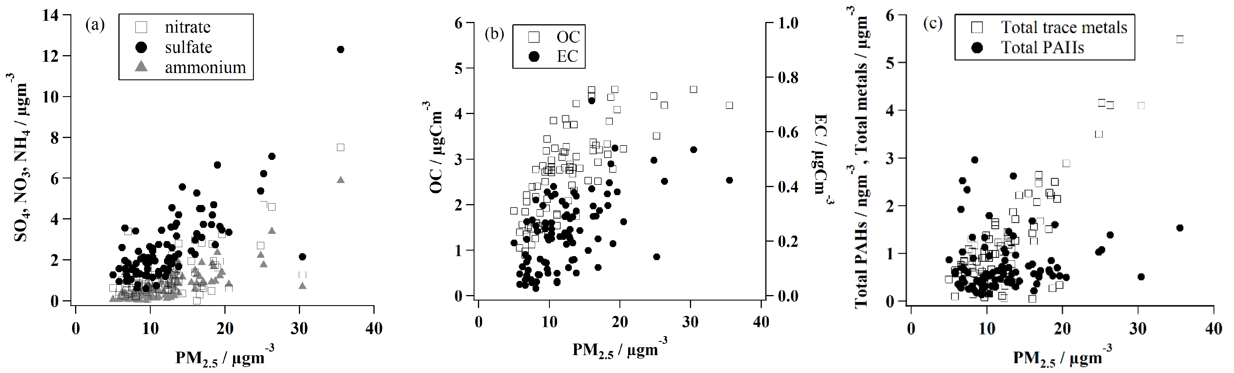
3.2. Correlation Plot

As mentioned earlier, the concentration variations in PM_2.5 and each chemical component are different from time to time, then the correlation was plotted for ionic components (sulfate, nitrate, ammonium), EC, OC, total trace metals, and total PAHs with respect to PM_2.5 concentration, which is shown in Figure 4. The concentrations of ionic components, EC, OC, and total metals increased with increasing PM_2.5 concentration, and their concentrations are considered to vary in the similar manner (Figure 4a–c). The EC and OC, both of which contain carbon, correlate to each other as shown in Figure 4b. Although we do not know the reason, both EC and OC seem not to increase when the PM_2.5 concentration is higher than 20 μgm⁻³. EC concentrations tend to be higher when wind speeds are low (not shown in Figures). This is presumably because local emissions become stagnant at low wind speeds. As shown in Figure 4c, PAHs tend to increase when the concentration of PM_2.5 is low. The variation in PAHs is different from PM_2.5 and other chemical components. The correlations revealed that PAHs have a slightly different trend from other chemical components.

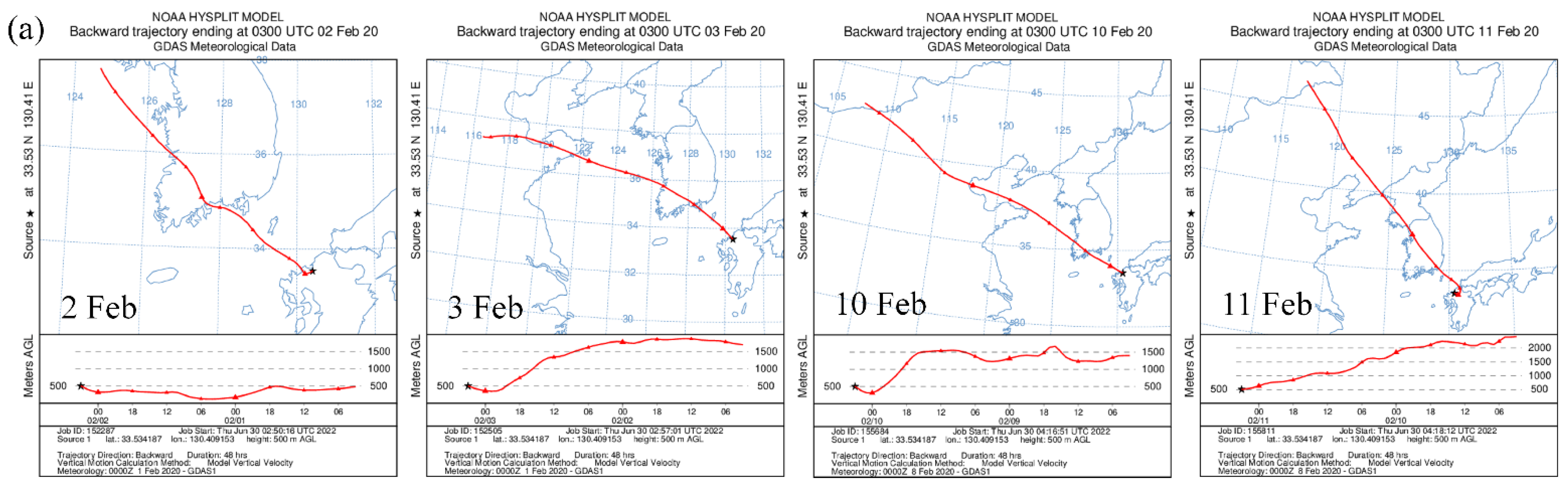
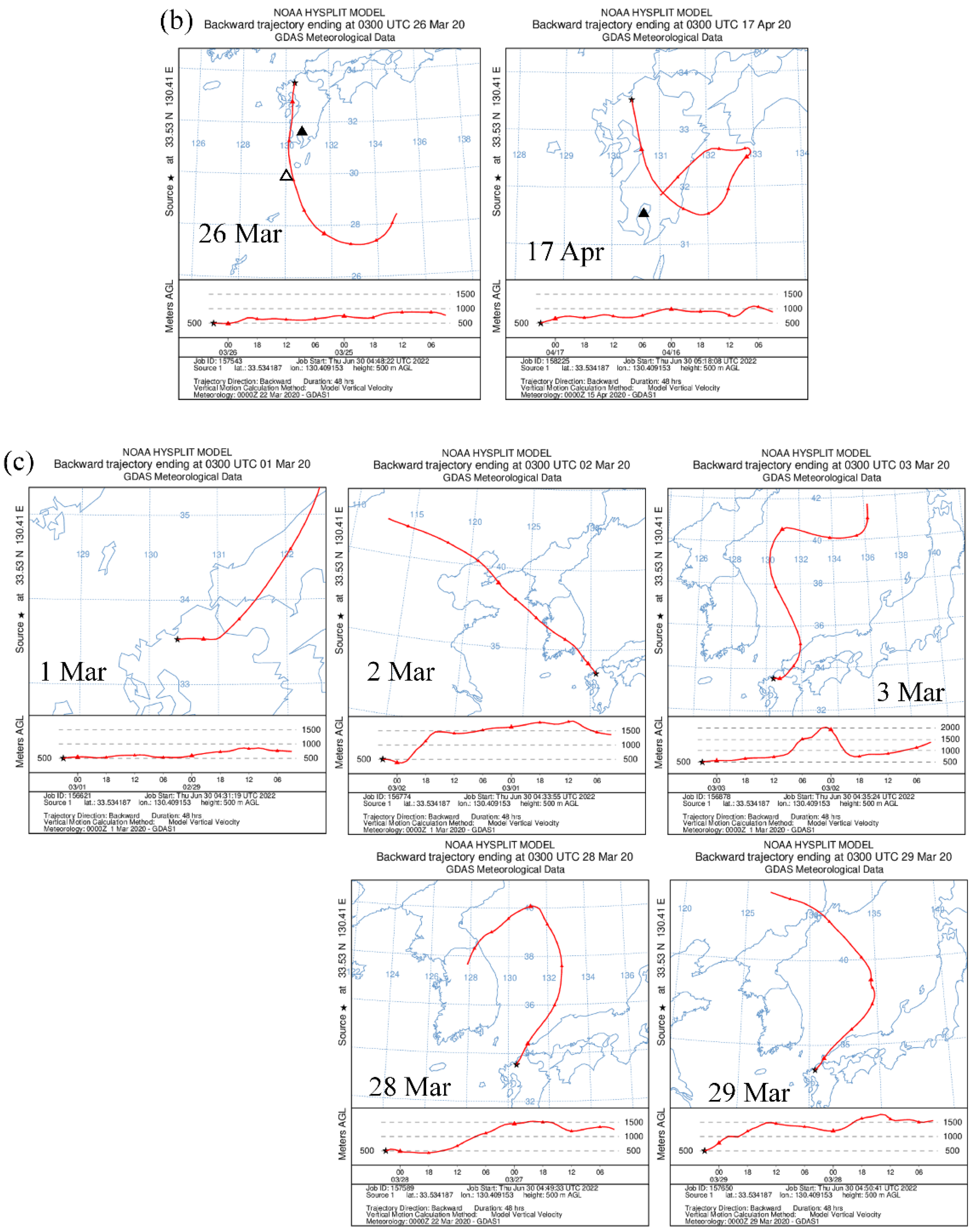
3.3. Days of High Concentration and Transport Paths

Human health is considered to be adversely affected when concentrations of PM and its components are high. In this section, we will examine the transport paths using back trajectory analysis when PM_2.5 and other chemical components are high.

The method used to extract high concentration days is as follows. The average and standard deviation were calculated for PM_2.5 and chemical components from February to April 2020. The average and standard deviation of PM_2.5, nitrate, sulfate, total ions, total PAHs, total metals, OC, EC, and ozone are 12.4 ± 5.50 µgm⁻³, 1.20 ± 1.13 µgm⁻³, 2.62 ± 1.73 µgm⁻³, 5.60 ± 3.71 µgm⁻³, 0.75 ± 0.56 ngm⁻³, 1.35 ± 1.02 µgm⁻³, 2.65 ± 1.34 µgm⁻³, 0.24 ± 0.25 µgm⁻³, and 37.8 ± 16.2 ppb, respectively. The high concentration days were defined as those greater than the average concentration plus one standard deviation. Then, the backward trajectory was calculated using HYSPLIT for each high concentration day for each component. The pathways along which air masses were transported were examined to investigate whether there was a relationship between high concentration and transport pathways.

Table 1. Days of high concentration of various chemical compositions in PM_2.5 and ozone in spring 2020. High concentration data is bolded. Ozone for 28–30 March were missing. SD means standard deviation (1σ).

Date	PM2.5/µgm−3	Nitrate/µgm−3	Sulfate/µgm−3	Total Ions/µgm−3	Total PAHs/ngm−3	Total Metals/µgm−3	OC/µgcm−3	EC/µgcm−3	O3/ppb
1 Feb	13.8	2.81	4.21	9.90	0.97	1.72	3.05	0.31	28.0
2 Feb	26.3	4.60	7.08	16.3	1.39	4.11	4.18	0.42	32.1
3 Feb	24.8	2.71	5.38	11.5	1.03	3.49	4.38	0.50	36.4
4 Feb	18.3	2.78	4.20	9.76	0.61	2.27	3.10	0.33	31.8
5 Feb	15.5	1.95	2.44	6.31	0.74	2.26	2.52	0.17	41.6
7 Feb	9.70	1.60	2.12	5.34	1.13	1.04	3.44	0.38	20.2
8 Feb	16.9	2.83	4.51	10.2	0.58	2.47	2.93	0.21	38.2
10 Feb	35.5	7.52	12.3	27.3	1.54	5.49	4.18	0.42	43.8
11 Feb	30.4	1.28	2.16	4.81	0.51	4.10	4.53	0.53	31.4
12 Feb	20.5	0.62	3.36	5.56	0.50	2.88	3.23	0.27	33.2
15 Feb	16.0	1.40	2.27	5.30	1.68	1.42	4.52	0.71	16.9
18 Feb	8.40	0.81	2.42	4.49	2.96	1.16	1.53	0.08	37.5
20 Feb	10.8	0.90	0.74	2.30	0.60	0.99	3.23	0.37	29.4
21 Feb	14.3	0.36	5.58	8.47	0.42	2.22	2.80	0.24	33.0
22 Feb	25.2	4.71	6.23	17.2	1.08	4.15	3.51	0.14	50.3
1 Mar	6.60	0.84	1.98	3.84	1.93	0.76	1.84	0.15	20.6
2 Mar	13.5	1.55	3.17	6.79	1.36	1.87	2.31	0.13	44.0
3 Mar	8.10	1.16	1.32	3.64	1.34	0.70	2.17	0.26	27.9
5 Mar	19.0	1.64	6.66	12.1	1.60	2.50	2.78	0.19	47.1
6 Mar	18.5	1.96	4.71	9.60	0.85	2.22	3.83	0.41	37.4
7 Mar	19.3	1.94	3.64	7.91	0.70	2.14	4.53	0.54	23.7
14 Mar	7.00	3.39	1.84	7.92	0.66	0.84	1.54	0.09	45.6
19 Mar	12.9	0.66	1.82	4.04	0.71	1.18	2.75	0.28	52.9
24 Mar	12.5	1.07	2.11	5.08	1.01	0.50	3.75	0.30	42.2
25 Mar	13.5	1.75	3.80	8.13	2.63	0.38	3.76	0.38	36.9
26 Mar	16.2	0.01	5.28	7.24	0.22	1.26	3.37	0.33	29.9
28 Mar	7.40	0.37	1.05	1.91	2.34	0.46	1.47	0.06	-
29 Mar	6.80	0.53	1.24	2.43	2.52	0.32	1.29	0.08	-
30 Mar	10.3	0.78	2.43	4.58	1.79	0.41	2.70	0.27	-
31 Mar	12.9	2.25	2.60	6.74	1.46	0.62	2.83	0.21	29.7
3 Apr	13.8	1.24	2.30	5.41	0.60	0.33	4.22	0.36	42.6
4 Apr	19.6	3.25	3.47	9.91	0.53	0.33	4.09	0.38	56.4
6 Apr	12.3	1.68	1.95	5.58	1.09	0.07	3.88	0.33	46.3
7 Apr	16.0	2.99	2.98	8.78	0.78	0.05	4.39	0.39	54.8
8 Apr	18.7	1.75	2.74	6.83	0.53	0.27	4.36	0.48	55.8
11 Apr	9.70	1.47	2.02	5.20	1.33	0.08	2.75	0.22	40.2
13 Apr	8.60	0.45	1.33	2.94	0.18	0.42	1.45	0.08	52.9
15 Apr	10.6	1.08	1.97	4.69	0.32	0.66	3.85	0.40	40.9
16 Apr	18.2	0.50	3.73	6.39	0.65	1.51	3.33	0.37	48.1
17 Apr	16.6	0.31	4.51	7.06	0.36	2.08	3.30	0.29	42.1
18 Apr	16.9	0.73	3.10	5.59	0.50	2.64	2.52	0.10	62.9
20 Apr	6.60	1.82	3.56	7.68	0.27	0.67	0.97	0.06	61.5
21 Apr	13.8	0.98	1.67	4.71	0.30	1.26	1.74	0.08	55.2
24 Apr	8.70	0.73	2.05	4.26	0.43	0.83	1.81	0.13	53.9
25 Apr	12.9	0.56	4.56	7.48	0.46	1.35	2.89	0.24	66.7
26 Apr	17.1	0.64	3.74	6.47	0.64	1.68	3.20	0.31	73.0
27 Apr	16.2	0.64	3.28	5.84	0.57	1.56	3.19	0.29	58.2
28 Apr	12.2	0.56	2.76	5.02	0.64	1.01	2.81	0.23	55.0
29 Apr	10.3	0.59	2.57	4.86	0.53	0.90	2.75	0.23	53.4
Average and SD of all days	12.4 ± 5.50	1.20 ± 1.13	2.62 ± 1.73	5.60 ± 3.71	0.75 ± 0.56	1.35 ± 1.02	2.65 ± 1.34	0.24 ± 0.25	37.8 ± 16.2

shows the days of high concentration of each component for February, March, and April, respectively. Each number is the respective concentration. All the concentrations for each component were high in some days, but in other cases, the concentration was high for a single or few components.

Typical examples of days with high concentrations for almost all components are 2–3 and 10–11 February. The maps of backward trajectory are shown in Figure 5a. The air masses reached Fukuoka from southern Korea, from the Shandong Peninsula through the northern East China Sea, or from northern China through the Yellow Sea. The backward trajectory suggests that transboundary air pollution from the Asian continent influences the Fukuoka air quality, which was seen before in Fukuoka [7,8,9]. Since Fukuoka is located in the western area of Japan, the seasonal monsoon prevails in the winter-spring season. The weather chart provided by the Japan meteorological Agency showed that a high-pressure system remained in the East China Sea area on 2–3 and 10–11 March, which is a typical atmospheric pressure pattern in winter season, and northerly wind prevails under this pattern. Then, the air pollutants emitted in the Asian continents are transported to Japan, especially in the west part of Japan [2,3,4,5,6,7,8,9]. However, local influences are also likely to affect the Fukuoka air quality. This is probable because the population in Fukuoka is about 1.5 million, and there are seaports and airports near the city in addition to the large industrial and commercial area. Therefore, the local emissions from the city itself affects the air quality in Fukuoka. The ozone shows diurnal variation and the wind direction indicates a sea-land wind pattern on those days [9,22,23], suggesting that the local emissions also affect the local air quality.

Typical examples of days when only sulfate was high were on 26 March and 17 April. The air mass moved northward from the south of the Kyushu area to reach Fukuoka, as shown in Figure 5b. This pattern probably affects the air quality in Fukuoka by increasing sulfate, which was generated by the oxidation of SO₂ from volcanoes such as Sakurajima and Suwanosejima. On 26 March, the back trajectory passed over both volcanoes. The weather chart shows that a high-pressure system remained in the south of Japan, which is a typical atmospheric pressure pattern for the southernly wind in the Kyushu area. A similar pattern was seen on 17 April. There are many active volcanoes in the Japanese island, and the air quality in the Kyushu area including Fukuoka is often affected by volcano eruptions, which brought sulfate in PM_2.5. Emissions from ships account for less than 5% of all PM_2.5 emission sources in the Kyushu area, which is very low [24].

Typical examples of the days when only PAHs concentration were high were seen on 1–3, 28–29 March. In the case of 1–3 March, ozone showed a diurnal variation and the wind direction shows a sea-land breeze pattern [9,22,23]. The weather chart shows that the atmospheric pressure pattern was in the transient state, in which there were low-pressure systems around Japan on 1–2 March and a high-pressure system moved from the Asian continent on 3 March. This pattern showed the prevailing influences of local emission. On the other hand, on 28–29 March, ozone concentrations did not decrease at night and did not show a diurnal pattern. In addition, the winds remained mostly northerly and wind speeds were at 6 to 8 ms⁻¹. The weather chart shows that high-pressure systems remained around at the Shangdon peninsula and the East China Sea. This pattern is presumably the prevailing influence of transboundary air pollution [9].

The patterns of ozone, wind direction, wind speed and the atmospheric pressure system on 1–3 March are different from 28–29 March, suggesting that the periods of 1–3 March are under the local prevailing influence and those of 28–29 March are under the influence of the transboundary air pollution. However, there are common features for the periods of 1, 3, 28–29 March, which include that the backward trajectory reached Fukuoka from Sea of Japan via Shimane and Yamaguchi prefectures as shown in Figure 5c. This suggests that these periods are affected by the local emissions, including local industries in Fukuoka and Kitakyushu [15] and ship emissions [25,26]. High PAHs concentrations may be brought due to the influence of local emission sources.

As shown above, some of chemical components, such as sulfate and PAHs, showed different concentration variations from PM_2.5 and other chemical components. This indicates that it is necessary to examine not only the health effects of PM_2.5, but also that of each chemical component. At the same time, it also indicates the need to study the source of each chemical component and its formation process in the atmosphere.

4. Conclusions

We have measured PM_2.5 and its chemical components in Fukuoka in spring 2020. The variations in chemical components are similar to that of PM_2.5 concentration except PAHs. We extract days with high concentrations. The paths taken by air masses were examined by backward trajectory using HYSPLIT. For the days with high concentrations for almost all components, the backward trajectory suggests that transboundary air pollution from the Asian continent influences the Fukuoka air quality in addition to the local sources. For high sulfate days, influences of active volcanoes, which emit SO₂, were suggested. For high PAHs days, the influence of local emissions in Fukuoka and Kitakyushu was suggested in addition to the transboundary air pollution. Some of chemical components showed the different concentration variations from PM_2.5 and other chemical components, which indicates that it is necessary to examine the health effects of each chemical component, and to study the source and formation processes of each chemical component in the atmosphere.

References

1. Ministry of the Environment (Japan). Reiwagannendo Taikiosenjokyohokokusho (Report of Air Pollution Condition in 2019); Ministry of the Environment, Government of Japan: Tokyo, Japan, 2019; p. 90. (In Japanese)
2. Takami, A.; Miyoshi, T.; Shimono, A.; Hatakeyama, S. Chemical composition of fine aerosol measured by AMS at Fukue Island, Japan during APEX period. Atmos. Environ. 2005, 39, 4913–4924. [Google Scholar] [CrossRef]
3. Takami, A.; Miyoshi, T.; Shimono, A.; Kaneyasu, N.; Kato, S.; Kajii, Y.; Hatakeyama, S. Transport of anthropogenic aerosols from Asia and subsequent chemical transformation. J. Geophys. Res. 2007, 112, D22S31. [Google Scholar] [CrossRef]
4. Sato, K.; Li, H.; Tanaka, Y.; Ogawa, S.; Iwasaki, Y.; Takami, A.; Hatakeyama, S. Long-range transport of particulate polycyclic aromatic hydrocarbons at Cape Hedo remote island site in the East China Sea between 2005 and 2008. J. Atmos. Chem. 2008, 61, 243–257. [Google Scholar] [CrossRef] [Green Version]
5. Sato, K.; Takami, A.; Irei, S.; Miyoshi, T.; Ogawa, Y.; Yoshino, A.; Nakayama, H.; Maeda, M.; Hatakeyama, S.; Hara, K.; et al. Transported and local organic aerosols over Fukuoka, Japan. Aerosol Air Qual. Res. 2013, 13, 1263–1272. [Google Scholar] [CrossRef] [Green Version]
6. Kaneyasu, N.; Yamamoto, S.; Sato, K.; Shimizu, A.; Hayashi, M.; Hara, K.; Kawamoto, K.; Okuda, T.; Hatakeyama, S. Impact of long-range transport of aerosols on the PM2.5 composition at a major metropolitan area in the northern Kyushu area of Japan. Atmos. Environ. 2014, 97, 416–425. [Google Scholar] [CrossRef]
7. Takami, A.; Miyoshi, T.; Irei, S.; Yoshino, A.; Sato, K.; Shimizu, A.; Hayashi, M.; Hara, K.; Kaneyasu, N.; Hatakeyama, S. Analysis of organic aerosol in Fukuoka, Japan using a PMF method. Aerosol Air Qual. Res. 2016, 16, 314–322. [Google Scholar] [CrossRef] [Green Version]
8. Yoshino, A.; Takami, A.; Sato, K.; Shimizu, A.; Kaneyasu, N.; Hatakeyama, S.; Hara, K.; Hayashi, M. Influence of trans-boundary air pollution on the urban atmosphere in Fukuoka, Japan. Atmosphere 2016, 7, 51. [Google Scholar] [CrossRef] [Green Version]
9. Yoshino, A.; Takami, A.; Hara, K.; Nishita-Hara, C.; Hayashi, M.; Kanyasu, N. Contribution of local and transboundary air pollution to the urban air quality of Fukuoka, Japan. Atmosphere 2021, 12, 431. [Google Scholar] [CrossRef]
10. Michikawa, T.; Ueda, K.; Takami, A.; Sugata, S.; Yoshino, A.; Nitta, H.; Yamazaki, S. Japanese nationwide study on the association between short-term exposure to particulate matter and mortality. J. Epidemiol. 2019, 29, 471–477. [Google Scholar] [CrossRef] [Green Version]
11. Kojima, S.; Michikawa, T.; Matsui, K.; Ogawa, H.; Yamazaki, S.; Nitta, H.; Takami, A.; Ueda, K.; Tahara, Y.; Yonemoto, N.; et al. Japanese Circulation Society with R (JCS-ReSS) Group, Relationship between fine particulate matter exposure and out-of-hospital cardiac arrest of cardiac origin: A nationwide registry-based Japanese study. SSRN Electron. J. 2019, 3, e203043. [Google Scholar] [CrossRef]
12. Integrated Science Assessment for Particulate Matter; USEPA: Washington, DC, USA, 2019.
13. Michikawa, T.; Yamazaki, S.; Ueda, K.; Yoshino, A.; Sugata, S.; Saito, S.; Hoshi, J.; Nitta, H.; Takami, A. Effects of exposure to chemical components of fine particulate matter on mortality in Tokyo: A case-crossover study. Sci. Total Environ. 2021, 755, 142489. [Google Scholar] [CrossRef] [PubMed]
14. Michikawa, T.; Morokuma, S.; Yamazaki, S.; Takami, A.; Sugata, S.; Yoshino, A.; Takeda, Y.; Nakahara, K.; Saito, S.; Hoshi, J.; et al. Exposure to chemical components of fine particulate matter and ozone, and placenta-mediated pregnancy complications in Tokyo: A register-based study. J. Expo. Sci. Environ. Epidemiol. 2022, 32, 135–145. [Google Scholar] [CrossRef] [PubMed]
15. Pham, K.-O.; Hara, A.; Zhao, J.; Suzuki, K.; Matsuki, A.; Inomata, Y.; Matsuzaki, H.; Odajima, H.; Hayakawa, K.; Nakamura, H. Different transport behaviors between Asian Dust and polycyclic aromatic hydrocarbons in urban areas: Monitoring in Fukuoka and Kanazawa, Japan. Appl. Sci. 2022, 12, 5404. [Google Scholar] [CrossRef]
16. Yang, L.; Tang, N.; Matsuki, A.; Takami, A.; Hatakeyama, S.; Kaneyasu, N.; Nagato, E.G.; Sato, K.; Yoshino, A.; Hayakawa, K. A comparison of particulate-bound polycyclic aromatic hydrocarbons long-range transported from the Asian continent to the Noto Peninsula and Fukue Island, Japan. Asian J. Atmos. Environ. 2018, 12, 369–376. [Google Scholar] [CrossRef]
17. Hayakawa, K.; Tang, N.; Xing, W.; Oanh, P.K.; Hara, A.; Nakamura, H. Concentrations and sources of atmospheric PM, polycyclic aromatic hydrocarbons and nitro polycyclic aromatic hydrocarbons in Kanazawa, Japan. Atmosphere 2021, 12, 256. [Google Scholar] [CrossRef]
18. PM2.5 Shitsuryo Nodo Oyobi Seibun Sokutei Kekka (Mass Concentration of PM2.5 and its Chemical Composition Analysis Data), Ministry of the Environment, Japan. Available online: https://www.env.go.jp/air/osen/pm/monitoring.html (accessed on 12 August 2022). (In Japanese).
19. Kakono Kisho Data (Past Weather Data), Japan Meteorological Agency. Available online: https://www.data.jma.go.jp/obd/stats/etrn/index.php (accessed on 12 August 2022). (In Japanese).
20. Stein, A.F.; Draxler, R.R.; Rolph, G.D.; Stunder, B.J.B.; Cohen, M.D.; Ngan, F. NOAA’s HYSPLIT atmospheric transport and dispersion modeling system. Bull. Am. Meteorol. Soc. 2015, 96, 2059–2077. [Google Scholar] [CrossRef]
21. Rolph, G.; Stein, A.; Stunder, B. Real-time Environmental Applications and Display sYstem: READY. Environ. Model. Softw. 2017, 95, 210–228. [Google Scholar] [CrossRef]
22. Fukuda, K.; Matsunaga, N.; Sakai, S. Behaviors of sea breeze above Fukuoka City. Annu. J. Hydraul. Eng. JSCE 2000, 44, 85–90. (In Japanese) [Google Scholar] [CrossRef]
23. Takashima, H.; Hara, K.; Nishita-Hara, C.; Fujiyoshi, Y.; Shiraishi, K.; Hayashi, M.; Yoshino, A.; Takami, A.; Yamazaki, A. Short-term variation in atmospheric constituents associated with local front passage observed by a 3-D coherent Doppler lidar and in-situ aerosol/gas measurements. Atmos. Environ. X 2019, 3, 100043. [Google Scholar] [CrossRef]
24. Chatani, S.; Shimadera, H.; Itahashi, S.; Yamaji, K. Comprehensive analyses of source sensitivities and apportionments of PM2.5 and ozone over Japan via multiple numerical techniques. Atmos. Chem. Phys. 2020, 20, 10311–10329. [Google Scholar] [CrossRef]
25. Wu, D.; Li, Q.; Ding, X.; Sun, J.; Li, D.; Fu, H.; Teich, M.; Ye, X.; Chen, J. Primary particulate matter emitted from heavy fuel and diesel oil combustion in a typical container ship: Characteristics and toxicity. Environ. Sci. Technol. 2018, 52, 12943–12951. [Google Scholar] [CrossRef] [PubMed]
26. Ando, H.; Miyata, O.; Imai, S.; Takahashi, C.; Niki, Y.; Xu, Z.; Nishio, S. Analysis of toxic substance in emission gas from marine diesel engine. Kaijo Gijutsu Anzen Kenkyu Hokoku 2011, 11, 111–126. (In Japanese) [Google Scholar]
Figure 1. Location of Fukuoka City.
Applsci 12 11400 g001
Figure 2. Time series of ozone, and meteorological data in spring 2020. (a) Ozone (O3), temperature, and solar radiation. (b) Wind speed and wind direction. (c) Data from 16 to 21 February for ozone, wind speed, and wind direction.
Applsci 12 11400 g002
Figure 3. Time series of mass concentrations of PM2.5 and its chemical component in spring 2020. (a) PM2.5, total ions, and total trace metals. (b) OC, EC, and total PAHs.
Applsci 12 11400 g003
Figure 4. Correlation plots of various chemical components with respect to PM2.5. (a) Sulfate, nitrate, and ammonium. (b) OC and EC. (c) Total trace metals and total PAHs.
Applsci 12 11400 g004
Figure 5. Backward trajectories of high concentration days for PM2.5, sulfate, and total PAHs. (a) February 2–3, and 10–11. (b) March 26 and April 17. Closed triangle: Sakurajima, open triangle: Suwanosejima. (c) March 1–3 and 28–29.
Applsci 12 11400 g005aApplsci 12 11400 g005b