Research on A Collaborative Control Strategy of An Urban Expressway Merging Bottleneck Area

Abstract

The conflict between the mainline and incoming traffic flow in the merging area of an urban expressway makes it easier to form a traffic bottleneck than the basic road section. When the merging bottleneck occurs, the overall efficiency is affected. This paper establishes an improved Cell Transmission Model (CTM) using Genetic Algorithms (GA) and Mean Absolute Percentage Error (MAPE) for parameter calibration and validation. Based on the joint optimization goal of efficiency and safety, a collaborative control strategy is established. The strategy is verified by VISSIM. The results show that the total travel time is reduced by 7.34%, and the total turnover is increased by 6.06% by applying the collaborative control strategy during the peak period. Therefore, the cooperative control strategy of the merging bottleneck proposed can improve the traffic state at the merging bottleneck and improve the efficiency and safety level of the expressway.

1. Introduction

As the highest-grade road in the urban road network system, urban expressways bear the function of the main skeleton of the road system. Compared with highways, expressways have a more concentrated distribution of entrances and exits, and adjacent entrances and exits are more closely connected with urban roads, resulting in more traffic conflicts on expressways than on highways [1]. Compared with urban arterial roads, expressways often bear more traffic demand due to their high design standards and closed traffic environment, resulting in a wider range of traffic bottlenecks and a faster diffusion rate.

The traffic control methods for expressways are mostly based on traffic flow models, and the simulation of expressway traffic state is realized by establishing models that conform to the changing expressway traffic flow trend. Compared with the microscopic and mesoscopic models, macroscopic models [2] focus on the aggregation behavior of traffic flow and involve three main parameters of interest: traffic density, speed, and flow. Macroscopic models define the traffic flow as a continuous fluid, which focuses on the continuous medium behavior, and simplifies the individual dynamic behavior between adjacent particles, such as lane changes and car-following. The characteristics of fewer parameters and fast calculation make it have great potential in the study of traffic flow management and control. With the development of the macroscopic continuous model LWR [3,4,5], classical macroscopic traffic flow models such as CTM [6] and METANET [7] have evolved. With the understanding of traffic flow, scholars have proposed improvements to the basic CTM to make it more in line with the traffic flow state under different scenarios. The improved CTM is applied to unmanned vehicles’ car-following model [8], vehicle routing [9], lane change overtaking [10], traffic congestion control strategy [11], freeway ramp control [12], and so on. The existing research on the improvement of macro traffic flow has shown little consideration of the complex traffic characteristics of the expressway merging bottleneck, which means the macro traffic flow model may have low simulation accuracy when applied to the related research of expressway merging bottleneck.

On the other hand, variable speed limit control of urban expressways has also attracted a lot of attention. Some scholars have studied the influence of variable speed limit control on traffic flow parameters. The research direction is the impact of variable speed limit control on traffic safety, road traffic performance, and traffic parameters. In terms of safety, this work [13] used the driving experiment method to prove that variable speed limit control can be used to improve traffic safety levels by collecting driver feedback. The research [14] used the accident risk model similar to [15] to evaluate the state of the road network and further proved that the variable speed limit control could improve the safety factor and road operation efficiency. In terms of traffic performance and traffic parameters, research by Zackor [15] found that variable speed limit control can maintain a certain equilibrium speed in each segment, thereby improving the speed inhomogeneity. The article [16] demonstrated in field tests that variable speed limit control can change the shape of the traffic flow fundamental diagram to control traffic flow at a high-density level before a sudden change, thereby improving freeway traffic performance during peak hours and easing traffic congestion. The work [17] used the traffic accident risk model to evaluate the effectiveness of variable speed limit control.

Due to the contradiction between traffic supply and demand, independent control methods are unable to adapt to the changing traffic flow characteristics in complex situations. In recent years, some scholars have begun to focus on the coordinated control strategy of on-ramp [18,19,20] and variable speed limit [21,22,23], with a view to improving traffic flow efficiency and accelerating the feedback rate. Model Predictive Control (MPC) [24,25] has achieved great success in the field of industrial control. Then, model predictive control is introduced to combine the macro traffic flow model, on-ramp control, and variable speed limit control for collaborative control design. However, most of the macro traffic flow models used are second-order METANET [26,27], which confirms the effectiveness of the collaborative control strategy.

At present, research on the bottleneck control of expressway merging areas has made some achievements. Scholars have improved the traditional macroscopic traffic flow model, ramp control, and variable speed limit control model and proposed control ideas based on different optimization objectives. However, there are still some problems in the improvement of the macroscopic traffic flow simulation model and the design of cooperative control strategy for expressway merging bottleneck, as follows:

• The expressway capacity often changes when the merging bottleneck occurs, and there are queues and overflows of on-ramp merging vehicles. Research on the improvement of macro traffic flow has little consideration of the complex traffic characteristics of expressway merging bottlenecks, which means the macro traffic flow model may have low simulation accuracy when applied to the research of expressway merging bottlenecks.
• At present, a lot of research has been obtained for the cooperative control of expressways, but most control strategies have little research on the mutual feedback between control algorithms and traffic flow models.
• The existing expressway control strategies based on the macro traffic model are mostly based on unilateral considerations, such as traffic efficiency, safety, environment, etc. The research on comprehensive optimization objective functions under multi-objective constraints needs to be improved.

This paper introduces the problem of urban expressway merging bottleneck area, focusing on the coordinated control of safety and efficiency. The existing expressway control strategies based on macroscopic traffic models are mostly based on unilateral considerations, and most control strategies have less research on the mutual feedback between control algorithms and traffic flow models. The main motivation for this research is to introduce the current methods for solving the cooperative control strategy of urban expressway merging bottleneck areas with the goal of efficiency and safety.

The rest of the paper is organized as follows. Section 2 proposes an improved CTM and gives the parameter calibration and validity test method. Section 3, MTFC-VSL (Mainline Traffic Flow Control-Variable Speed Limit) is used for speed limit control, PI-ALINEA is used for ramp merging control, and MPC is used to establish a merging bottleneck cooperative control model. Section 4 takes Xi’an Expressway in Shaanxi, China as an example to build a VISSIM simulation model to analyze the control effect of the collaborative control strategy. Section 5 presents the conclusion and suggestions for future work.

2. Improved CTM and Parameter Calibration, Validity Verification

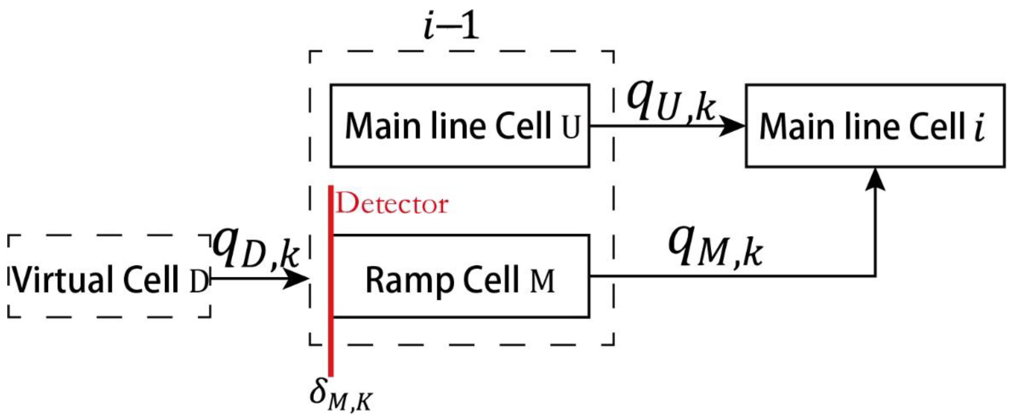
2.1. Cell Space Division Improvement

In the basic CTM, the road is divided into several equidistant cells, and the research time is also divided into equal time steps. The cell length is fixed and not less than the single-time step vehicle driving distance in the free flow state. However, the basic CTM has defects in cell length division, basic diagram relation of merging cells, and cell description of the on-ramp. In this paper, the spatial division method in the basic CTM is improved, and the cell state representation variable is changed, so the density is used to describe the cell traffic state so that the cell length in the model can be changed according to the actual conditions of the expressway. The variable-length CTM is shown in Figure 1.

In the variable-length CTM:

$${\rho }_{i,k+1}={\rho }_{i,k}+\frac{\mathsf{\Delta }t}{{\lambda }_i\cdot l_i}\left(q_{i,k}-q_{i+1,k}\right)$$

(1)

where ${\rho }_{i,k}$ represents average density of cell $i$ at the beginning of kth time step ($\mathrm{pcu}/\mathrm{km}/\ln$). $q_{i,k}$ represents traffic flow into cell $i$ in kth time step ($\mathrm{pcu}/\mathrm{h}$). ${\lambda }_i$ represents number of lanes in cell $i$. $l_i$ represents length of cell $i$. $\mathsf{\Delta }t$ represents time step, which should satisfy $\mathsf{\Delta }t\le \min \left(l_i/v_f\right)$ in variable-length CTM.

Formula (1) is a flow conservation equation that describes the cell state update with traffic flow density and traffic flow rate. At this time, the sending and receiving capabilities of the cell also use the sending rates $s_{i,k}$($\mathrm{pcu}/\mathrm{h}$) and the receiving rate $r_{i,k}$($\mathrm{pcu}/\mathrm{h}$) to replace the number of vehicles:

$$s_{i,k}=\min \left\{{\lambda }_i{v}_f{\rho }_{i,k},{\lambda }_i{q}_m\right\}$$

(2)

$$r_{i,k}=\min \{{\lambda }_i{q}_m,{\lambda }_{i}w\left({\rho }_j-{\rho }_{i,k}\right)\}$$

(3)

where $v_f$ represents the free-flow speed of cell ($\mathrm{km}/\mathrm{h}$). ${\rho }_j$ represents traffic flow average congestion density in cell ($\mathrm{pcu}/\mathrm{km}$). $q_m$ represents single lane capacity in cell ($\mathrm{pcu}/\mathrm{h}$). $w$ represents the speed value of the blocking wave propagating backward along traffic flow under high density, $w<v_f$.

Formula (1) can be derived as:

$$q_{i,k}=\min \left\{s_{i-1,k},r_{i,k}\right\}$$

(4)

where $s_{i-1,k}$ represents sending ability of upstream cell $i-1$.

Formulas (1)–(4) are basic models described by traffic flow density and traffic flow rate instead of vehicles’ numbers in the variable-length CTM.

Transform the basic CTM:

• Merging cell i can receive the maximum number of upstream mainline vehicles and ramp cells can send.

$$\{\begin{array}{c}{q}_{U,k}=s_{U,k}\\ q_{M,k}=s_{M,k}\\ q_{i,k}=q_{U,k}+q_{M,k}=s_{U,k}+s_{M,k}\end{array} , r_{i,k}\ge s_{U,k}+s_{M,k}$$

(5)

2.

Merging cell i cannot receive the maximum number of upstream mainline vehicles and ramp cells can send.

$$\{\begin{array}{c}{q}_{U,k}=\mathrm{mid}\left\{s_{U,k},r_{i,k}-s_{M,k},r_{i,k}\cdot \left(1-\theta \right)\right\}\\ q_{M,k}=\mathrm{mid}\left\{s_{M,k},r_{i,k}-s_{U,k},r_{i,k}\cdot \theta \right\}\\ q_{i,k}=q_{U,k}+q_{M,k}=r_{i,k}\end{array} , r_{i,k}<s_{U,k}+s_{M,k}$$

(6)

where $q_{U,k}$ represents the number of vehicles entering the upstream mainline. $q_{M,k}$ represents the number of vehicles entering the upstream ramp. $q_{i,k}$ represents the number of vehicles flowing into cell $i$. $s_{U,k}$ represents sending ability of upstream mainline cell.$s_{M,k}$ represents sending ability of upstream ramp cell. $r_{i,k}$ represents receiving ability.

Assuming that the number of vehicles flowing into the mainline cell L is $q_{L,k}$, the number of vehicles flowing into the ramp cell is $q_{M,k}$, and the diverging rate of the ramp cell is $\beta$, the diverging model is transformed into:

$$\{\begin{array}{c}{q}_{i+1,k}=\min \left\{s_{i,k},r_{L,k}/\left(1-\beta \right),r_{M,k}/\beta \right\}\\ q_{L,k}=q_{i+1,k}\cdot \left(1-\beta \right)\\ q_{M,k}=q_{i+1,k}\cdot \beta \end{array}$$

(7)

With variable-length cells, Formulas (1) and (4)–(6) constitute the merging CTM described by density and flow rate. Formulas (1), (4) and (7) constitute the diverging CTM.

2.2. Improve Merging Cell Basic Diagram

Improve the basic diagram of merging cell $i$, as shown in Figure 2.

In this figure, $q_{m_1}$ and $q_{m_2}$ represent the capacity of a single lane in cell $i$ before and after the sudden drop of capacity, $w^{\prime }$ represents the speed of shock wave after the sudden drop of capacity, ${\rho }_m$ represents the critical density when the sudden drop of capacity occurs. For the merging cell $i$, due to the double-value phenomenon of its capacity, its sending rate and receiving rate need to be updated as:

$$s_{i,k}=\{\begin{array}{c} {\lambda }_i{v}_f{\rho }_{i,k} {\rho }_{i,k}<{\rho }_m\\ \min \left\{{\lambda }_i{v}_f{\rho }_{i,k},{\lambda }_i{q}_{m_2}\right\} {\rho }_{i,k}\ge {\rho }_m\end{array}$$

(8)

$$\{r_{i,k}\mathrm{g}=\{\begin{array}{c}\min \left\{{\lambda }_{i}w\left({\rho }_j-{\rho }_{i,k}\right),{\lambda }_i{q}_{m_1}\right\} {\rho }_{i,k}<{\rho }_m\\ \min \left\{{\lambda }_i{w}^{\prime }\left({\rho }_j-{\rho }_{i,k}\right),{\lambda }_i{q}_{m_2}\right\} {\rho }_{i,k}\ge {\rho }_m\end{array}$$

(9)

Formulas (8) and (9) are the sending and receiving capacities of merging cell $i$ into the updating merging model, which can improve the sudden drop of bottleneck capacity.

2.3. Update Entrance Ramp Status

When there is congestion on the ramp, the arrival rate on the detection line will decrease, which makes the CTM wrongly judge this phenomenon as a decrease in ramp traffic demand. At the same time, the ramp cell M only serves as a state update tool for the merging cell $i$ and loses track of its own traffic state. Based on the above analysis, this paper proposes improvements to the defects of ramp cells.

In Figure 3, it is assumed that there is a virtual initial cell D in front of the on-ramp cell M, which can be regarded as a collection of roads connected to the on-ramp and the urban roads along it. Therefore, the flow rate $q_{D,k}$ that leaves the cell D and flows into the cell M within the kth time step is the vehicle arrival rate ${\delta }_{M,k}$ detected by the on-ramp detection line, and the conservation law of the on-ramp cell M can be defined by referring to Equation (1):

$${\rho }_{M,k+1}={\rho }_{M,k}+\frac{\mathsf{\Delta }t}{{\lambda }_M\cdot l_M}\left(q_{D,k}-q_{M,k}\right)$$

(10)

The formula is the state update formula of the ramp cell, in which $q_{D,k}$ has been calibrated by the vehicle arrival rate ${\delta }_{M,k}$ detected on the detector. Therefore, in order to update the implementation (10) in each time step, the $q_{M,k}$ value needs to be determined. From Equation (5) to (6), it can be seen that $q_{M,k}$ is determined by the transmission capability $s_{M,k}$ of cell M, the transmission capability $s_{U,k}$ of cell U and the receiving capability $r_{i,k}$ of cell $i$, where $s_{U,k}$ and $r_{i,k}$ can be calibrated by Equations (2) and (8) respectively. For the transmission capability $s_{M,k}$ of ramp cell, the actual traffic demand of ramp is used to replace the detection arrival rate so as to ensure the flow conservation on cell M and avoid the misjudgment of ramp traffic demand by CTM. The expression is as follows:

$$s_{M,k}=\min \left\{{\lambda }_M{v}_f{}^{\prime }{\rho }_{M,k},{\lambda }_M{q}_m{}^{\prime }\right\}$$

(11)

where ${\lambda }_M$ represents number of lanes on ramp cell M. $v_f{}^{\prime }$ represents free-flow speed on ramp cell M (km/h). ${\rho }_{M,k}$ represents average traffic density of cell M at the beginning of kth time step (pcu/km/ln). $q_m{}^{\prime }$ represents single lane capacity of cell M.

2.4. Model Parameter Calibration and Validity Test

In the improved CTM, the parameters to be calibrated are: $v_f$ (mainline cell free- flow speed), $v_f{}^{\prime }$ (ramp cell free-flow speed), $q_m$ (mainline ordinary cell capacity), $q_m{}^{\prime }$ ( ramp cell capacity), $q_{m_1}$ and $q_{m_2}$ (merging cell capacity), ${\rho }_m$ (cell key density), $w$ (cell congestion wave speed), $w^{\prime }$ (merging cell capacity after the sudden drop of congestion wave speed), etc., and the capacity reduction rate at the merging bottleneck is set as $\alpha$. Then $q_{m_2}$ and $w^{\prime }$ can be simplified as $q_{m_1}\left(1-\alpha \right)$, $w\left(1-\alpha \right)$.

The simulation-actual value deviation sum of squares of flow and speed is selected as the solution target. The joint objective function is expressed as follows:

$$s_{M,k}=\min \left\{{\lambda }_M{v}_f{}^{\prime }{\rho }_{M,k},{\lambda }_M{q}_m{}^{\prime }\right\}$$

(12)

where $N_1$ represents number of cells in the model. $N_2$ represents the number of time steps in the model. ${\mu }_{i,k}$ represents the standardized simulation speed value of the kth time step cell $i$. ${\mu }_{i,k}{}^r$ represents the standardized measured speed of the kth time step cell $i$. ${\phi }_{i,k}$ represents standardized flow value of the kth time step cell $i$. ${\phi }_{i,k}{}^r$ represents standardized measured flow value of the kth time step cell $i$.

Assuming that the parameter vector of the model to be calibrated is $Z^T=\left(v_f,q_m,w,\alpha \right)$, it is necessary to determine the appropriate optimization algorithm to solve the optimal parameters that make the objective function meet the set requirements. Genetic Algorithms (GA) have the advantages of fast convergence and boundary conditions when dealing with multi-feasible solution search problems [20].

After the model parameters are calibrated, the accuracy of the traffic flow simulation is analyzed by Mean Absolute Percentage Error (MAPE). It means the mean value of the ratio of the difference between predicted and actual results to the actual value. The effectiveness of the model is evaluated according to the MAPE value. The effectiveness increases with the decrease of MAPE. This paper considers that the model simulation results are better when the MAPE value is less than 10%. Select speed, and flow as the evaluation object, the validity index calculation expression are as follows:

$$\mathrm{MAPE}=\frac{1}{2}·\frac{1}{N_1}·\frac{1}{N_2}\left[{\displaystyle \sum }_{i=1}^{N_1}{\displaystyle \sum }_{k=1}^{N_2}\frac{|v_{i,k}-v_{i,k}{}^r|}{|v_{i,k}{}^r|}+{\displaystyle \sum }_{i=1}^{N_1}{\displaystyle \sum }_{k=1}^{N_2}\frac{|q_{i,k}-q_{i,k}{}^r|}{|q_{i,k}{}^r|}\right]$$

(13)

where $v_{i,k}$ represents the simulation speed value of the kth time step cell $i$. $v_{i,k}{}^r$ represents measured speed of the kth time step cell $i$. $q_{i,k}$ represents simulation flow value of the kth time step cell $i$. $q_{i,k}{}^r$ represents measured flow value of the kth time step cell $i$.

3. Construction of Collaborative Control Strategy for Expressway Merging Bottleneck

3.1. Basic Thinking

There are two types of control algorithms widely used in industrial practice: PID and MPC. MPC adopts a feedback control structure based on a predictive model, which has better applicability when applied to expressway traffic flow control with obvious nonlinearity, large time-varying uncertainty, and difficult solution. This paper selects MPC as a collaborative control algorithm. The algorithm’s structure is shown in Figure 4.

When the MPC is applied to the expressway merging bottleneck, the process can be divided into four steps: prediction, effect evaluation, optimization, and control, as shown in Figure 5.

3.2. Objective Function

The urban expressway control target is generally composed of efficiency and safety. For the traffic efficiency target, we use the comprehensive index of total travel time and total turnover as the efficiency control target function. The expression is as follows:

$$\begin{array}{c}{J}_1={\displaystyle {\displaystyle \sum }_{k=1}^T}\mathsf{\Delta }t[{\displaystyle {\displaystyle \sum }_{i=1}^N}({\rho }_{i,k}{\lambda }_i{l}_i-{\delta }_N{\rho }_{i,k}{v}_{i,k}{\lambda }_i{l}_i)\\ +{\displaystyle {\displaystyle \sum }_{i=1}^M}({\omega }_{i,k}-{\delta }_M{\omega }_{i,k}{v}_{i,k})]\end{array}$$

(14)

where ${\rho }_{i,k}$ represents the average density of segment $i$ at the kth sampling period. ${\lambda }_i$ represents the number of lanes on segment $i$. $l_i$ represents the length of segment $i$. $v_{i,k}$ represents the average speed of segment $i$ in the kth sampling period. $T$ represents the predicted number of time intervals. $N$ represents the number of expressway segments. $M$ represents the number of entrance ramps. ${\omega }_{i,k}$ represents the number of queuing vehicles at the entrance ramp $i$ at the kth sampling period. ${\delta }_N,{\delta }_M$ represents the dimensional balance coefficient, which balances the influence of each index on the objective function, is taken as $1/v_f$. $\mathsf{\Delta }t$ represents a single sampling interval.

For safety, considering the complexity and uncertainty of traffic conflicts and accidents, the prediction of serious conflicts is selected as the objective, and the objective function expression is as follows [19]:

$$J_2={\displaystyle \sum }_{k=1}^T{\displaystyle \sum }_{i=1}^N\begin{array}{c}[591.634-14.872{\rho }_{i,k}+1.625\Delta v_{i,m}+\\ 1.638SVT+0.877SVD]\end{array}$$

(15)

$$SVT=|v_{i,k+1}-v_{i,k}|$$

(16)

$$SVD=|v_{i,k}-v_{i-1,k}|$$

(17)

where $\Delta v_{i,m}$ represents speed difference between mainline and ramp. $SVT$ represents the speed difference between adjacent periods of the same segment of mainline, that is the time speed difference. $SVD$ represents the speed difference between adjacent segments of the mainline in the same period, that space speed difference.

Before determining the comprehensive control objective function, due to the dimensional difference between the efficiency objective and the safety objective, the value of each objective function needs to be dimensionless processing. The processing method adopts the (0,1) interval method. The expression is as follows:

$$J_i{}^{\prime }=\frac{\left(J_i-J_{i,\min }\right)}{\left(J_{i,\max }-J_{i,\min }\right)}$$

(18)

where $J_i$ represents a dimension value. $J_i{}^{\prime }$ represents a dimensionless value. $J_{i,\max }$ represents the maximum dimension value. $J_{i,\min }$ represents the dimension minimum dimension value.

An objective function based on safety and efficiency is obtained:

$$J=J_1{}^{\prime }+J_2{}^{\prime }$$

(19)

3.3. Strategy Design

The improved CTM is used as the prediction unit of the traffic flow state, MTFC-VSL for mainline and PI-ALINEA for ramp are used as the control unit of the traffic system, and the traffic safety and efficiency are used as the joint optimization objectives to build the merging bottleneck cooperative control strategy. The main process is as follows in Figure 6.

4. An Illustrative Example

4.1. Simulation Platform Construction

This paper selects as the survey object the urban expressway of Xi’an City, Shaanxi Province, China. Comparing the second ring road and the third ring road in the Xi’an loop line system, it is found that compared to the third ring road, the second ring road has more and denser entrances and exits on both sides, and the closure is poor, which is closer to the urban trunk road in function. In contrast, the third ring road is more in line with the functional positioning of the urban expressway. Therefore, the survey objects matching the research of this paper are selected on the third ring road. Select the evening peak survey data as research data. As shown in Figure 7, Figure 8 and Figure 9, the total length of the investigated segment is 2.46 km. The distance between the two merging areas is about 396 m, and the distance between the merging area and the downstream diverging area is about 200 m. The first merging area is Guang’an Road (expressway), which is connected to the mainline of the East Third Ring Road through the entrance ramp of Andi Interchange. The second merging area is the East Third Ring Road, which is connected to the main line through the entrance ramp. The merging area adopts parallel acceleration lanes. VISSIM is selected to simulate the experimental road to obtain the real-time traffic flow data required for the control strategy, and the effect of the control strategy is evaluated according to the output data of each detector.

Based on the two principles of diverging area and merging area as a separate segment and similar road conditions in each basic segment, the experimental segment is divided. Figure 10 shows the division of the experimental segment and its cell division results. The expressway mainline is divided into nine segments, of which Cell3 and Cell6 are merging segments, Cell8 is a diverging segment, Merge1 and Merge2 represent the entrance ramp segments of the two merging areas, and Diverge is the diverging ramp segment.

The simulation needs to accurately reflect the road operation and provide a reliable experimental basis for the effective evaluation of the subsequent control strategy. In order to avoid congestion caused by the insufficient capacity of the mainline, this paper considers the running state of the mainline traffic flow without a ramp and finds that it is not the congestion caused by excessive traffic flow of the mainline. Therefore, the relevant parameters in VISSIM software should be calibrated according to the actual operation of road traffic. As shown in Figure 11, the simulation road network is constructed according to the actual road conditions. According to Figure 10, the simulation road section is divided into different segments. Data detectors are set in each segment and queuing, and flow detectors are set at the entrance ramp. Based on the measured data on Friday, December 11, 2020, the simulation road path decision, traffic rules, vehicle composition, traffic flow, etc., are input. The simulation duration is set to 2 h, and the peak hours are 1800 s–5400 s. As shown in Figure 12, the split path decision point is set at the starting point of the split zone, and the split ratio is set to 0.15; according to the actual observation situation, the conflict area at the connection between the entrance ramp and the mainline is set as the alternate traffic rule; according to the actual data statistics, the vehicle composition of the mainline and the entrance ramp is shown in

Table 1. Simulation vehicle composition input.

	Cars	Trucks	Buses
Mainline	86%	8%	6%
Ramp	91%	6%	3%

. In order to simulate the uneven arrival characteristics of the ramp vehicles, the flow type is set to random arrival. The merging area 2 flow is larger than the merging area 1, and the interference to the mainline is stronger. The traffic flow input into the simulation system through the initial section of the mainline and the two entrance ramps in each period is shown in Figure 13.

The simulation segment needs to reflect the road operation and provide a reliable experimental basis for the subsequent control strategy. As shown in Figure 14, the flow and speed data obtained by each segment detector after inputting the measured traffic demand in each period into VISSIM are output.

4.2. Parameter Calibration

According to the above, the parameters to be calibrated in the improved CTM are the free flow speed and capacity of the mainline and ramp cells, the congestion wave propagation speed, and the decline rate of the merging cell’s capacity. Based on the detector data of each segment uncontrolled output by VISSIM (sampling interval 6 s, $\mathsf{\Delta }t\le \min \left(l_i/v_f\right)$), GA is used as the optimization algorithm, and the sum of squares of deviation between flow and speed is taken as the solution target to optimize the parameters of the improved CTM prediction model. The initial boundary values of each genetic variable parameter are shown in

Table 2. Parameter range of genetic variables.

Variable Name	Meaning	Boundary
$v_f$	Mainline free flow speed	[65 km/h,75 km/h]
$v_f{}^{\prime }$	Ramp free flow speed	[45 km/h,55 km/h]
$q_m$	Mainline Capacity of single lane	[1800 pcu/h,2200 pcu/h]
${q_m}^{\prime }$	Ramp capacity of single lane	[1600 pcu/h,2100 pcu/h]
$w$	Congested wave speed	[10 km/h,18 km/h]
$\alpha$	Capacity decline rate	[7%,15%]

.

After setting the initial range of genetic variables, python is used to realize the procedural expression of improved CTM and GA optimization solution. The parameter values of the genetic algorithm are shown in

Table 3. Genetic algorithms’ population parameter value.

Algorithm Parameters	Parameter Value
Population size $P$	100
Maximum number of iterations $G$	200
Crossover probability $P_x$	0.7
Mutation probability $P_{var}$	0.1
Fitness function Fitness ()	$\frac{1}{\min J_{v,q}}$

.

After the parameter setting, the genetic algorithm optimization operation is performed, as shown in Figure 15 and

Table 4. Improved CTM parameter calibration results.

Parameter Calibration
${\mathit{v}}_{\mathit{f}}$ (km/h)	${\mathit{v}}_{\mathit{f}}{}^{\prime }$ (km/h)	${\mathit{q}}_{\mathit{m}}$ (pcu/h)	${{\mathit{q}}_{\mathit{m}}}^{\prime }$ (pcu/h)	$\mathit{w}$ (km/h)	${\mathit{w}}^{\prime }$ (km/h)	${\mathit{\rho }}_{\mathit{m}}$ (pcu/km.ln)	$\mathit{\alpha }$ %
70.2	49.4	2095	1807	16.7	14.4	32.3	13.7

, which is the iterative result of the improved CTM parameter calibration.

Under the optimal parameters obtained by satisfying the maximum iterations, the temporal and spatial distribution of the average absolute percentage error between the speed-flow data output by the improved CTM and the detector data for the Cell1-Cell9 segments at each sampling interval is shown in Figure 16. From the results of error distribution, it can be seen that the error of the Cell1-Cell2 segment is at a good level (within 10%) in the whole prediction period. Due to the interference of the entrance ramp, the traffic conditions on the Cell3-Cell6 segment are more complicated, and the error is slightly higher than in other segments. The error increases greatly during the peak period, and the error value is up to 14%, but the error is at an acceptable level in most periods. The Cell7-Cell9 segment was at a good level during the flat peak period (within 10%), and its error values were within 10% for most of the peak period. In general, the mean absolute percentage error (MAPE) of the prediction results of the improved CTM in the whole prediction period is about 8.6%, and the prediction results of the traffic flow on each segment are within the acceptable range, and there is no obvious deviation, indicating that the improved CTM has high accuracy in simulating and predicting the expressway merging bottleneck.

For the control algorithm in the cooperative control strategy, the parameter calibration results are shown in

Table 5. Control model parameter calibration results.

Parameter	Meaning	Calibration Value
$K_P^{\prime }$	MTFC-VSL Target flow proportional gain	100
$K_I^{\prime }$	MTFC-VSL Target flow integral gain	15
$K_I$	MTFC-VSL Rate-limiting integral gain	6 × 10−3
$D^{+}$	PI-ALINEA Upper limit of adjustment value	40
$D^{-}$	PI-ALINEA Lower limit of adjustment value	−10
$\gamma$	Smooth coefficient of mainline expected occupancy	0.8
$K_P$	PI-ALINEA Proportional gain	80
$K_R$	PI-ALINEA Feedback gain	40
$L_{\max }$	Maximum ramp queue length	100

.

Parameter calibration of MPC in cooperative control strategy is shown in

Table 6. MPC parameter calibration results.

Parameter Calibration
Sampling Period $\mathbf{\Delta }\mathit{t}$ (s)	Control Cycle $\mathbf{\Delta }\mathit{T}$ (s)	Predictive Time Length ${\mathit{N}}_{\mathbf{p}}$ (Min)	Control Time Length ${\mathit{N}}_{\mathbf{C}}$ (min)
10	60	10	8

.

4.3. Effect Evaluation

In Figure 17, the simulation results are output after the cooperative control strategy is turned on at the two merging areas on the VISSIM. Comparing the changes of the expressway traffic flow state under the uncontrolled state shown in Figure 14, it can be seen that the traffic flow operation of each segment under the cooperative control is obviously more stable, and the space-time spread range of congestion is significantly reduced. From the time point of view, the speed of the Cell6 segment decreased to about 40 km/h at about 41 min, and the state began to spread to the upstream segment. At 83 min, each segment has returned to a smoother operating state, and the duration of congestion is significantly reduced compared with the uncontrolled state (36 min~100 min). From the spatial point of view, the flow distribution of each segment is more uniform during the peak period. Compared with the uncontrolled state, the traffic flow speed of the initial segment Cell1 remains above 50 km/h throughout the peak period, indicating that the spatial propagation range of congestion is reduced under coordinated control. In terms of the merging bottleneck control effect, the minimum traffic flow speed is 37.3 km/h (27.6 km/h uncontrolled), which is smaller than that of the uncontrolled state, indicating that the cooperative control strategy proposed in this paper has a good effect in controlling the merging bottleneck.

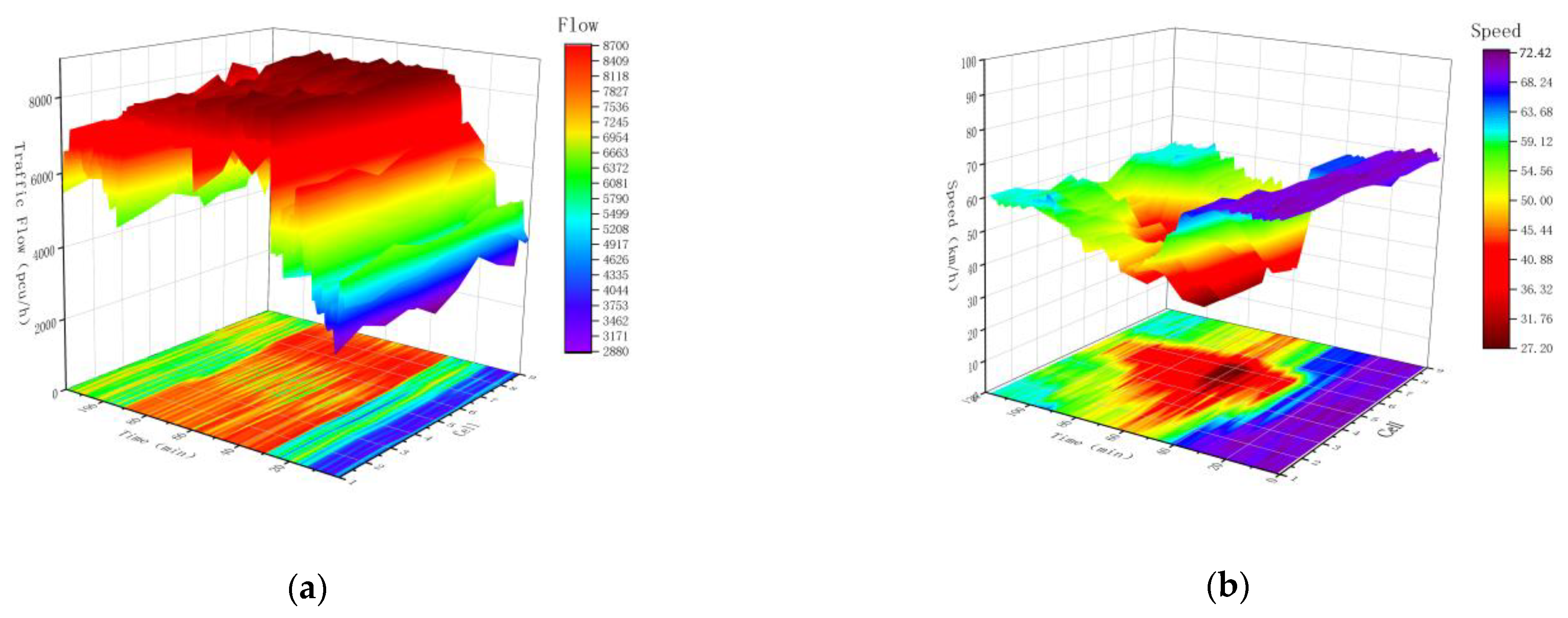
4.3.1. Merging Bottleneck Control Effect Analysis

In order to further analyze the effect of the control strategy in improving the operation efficiency, the traffic flow state parameters (flow, density, speed) under uncontrolled state and cooperative control state are output, as shown in Figure 18.

It can be seen that when there is no control, the sudden drop in traffic capacity in the two merging areas near 36 min occurs. At this time, the traffic density in the merging area rises rapidly, and the speed drops sharply, which becomes the merging bottleneck restricting the operation of expressway traffic flow. After the cooperative control is opened, the traffic flow of the main line and ramp into the region is limited under the variable speed limit and ramp merging control. The maximum value of the traffic flow in the two merging areas is smaller than that in the uncontrolled state. Although the traffic capacity decreases, the magnitude of the decrease is significantly reduced, and the change is more moderate. The traffic flow is maintained at a high level during the peak period, and the traffic flow operation state is significantly improved compared with the uncontrolled state.

4.3.2. Traffic Efficiency Improvement Analysis

(1)

Operational efficiency comparison

VISSIM outputs the operation efficiency indexes of merging area 1 and merging area 2 under no control and cooperative control during the simulation period, as shown in

Table 7. Comparison of operation efficiency before and after control of merging area 1.

	Mainline			Ramp
Evaluating Indicator	Uncontrolled	Cooperative Control	Optimized Ratio	Uncontrolled	Cooperative Control	Optimized Ratio
Total travel time (veh·h)	103.980	94.600	+9.02%	9.280	10.109	−8.93%
Total delay time (veh·km)	11.956	10.272	+14.09%	4.759	5.141	−8.04%
Maximum queue length (m)	293	237	+19.11%	44	47	−6.82%
Stop times (veh·times)	266	239	+10.15%	144	157	−9.03%

and

Table 8. Comparison of operation efficiency before and after control of merging area 2.

	Mainline			Ramp
Evaluating Indicator	Uncontrolled	Cooperative Control	Optimized Ratio	Uncontrolled	Cooperative Control	Optimized Ratio
Total travel time (veh·h)	122.690	99.311	+19.06%	18.887	15.874	+15.95%
Total delay time (veh·km)	30.893	20.070	+35.03%	13.082	8.739	+33.20%
Maximum queue length (m)	368	268	+27.17%	89	67	+24.72%
Stop times (veh·times)	359	307	+14.48%	475	369	+22.48%

Tables may have a footer. In the optimized ratio, ‘+’ indicates the degree of improvement, and ‘−’ indicates the degree of deterioration.

(In order to avoid the influence of the control of merging area 2 on the operation efficiency of merging area 1, when the cooperative control of merging area 1 is turned on, the control system of merging area 2 is closed, which is the same as that of merging area 2). It can be seen that for merging area 1, after the coordinated control is applied, the operation efficiency indexes of the main line are improved to a certain extent, and the ramp operation efficiency decreases, but the decrease of each index is within 10%. For merging area 2, the traffic operation at the mainline and ramp is more stable than that in the uncontrolled state after applying cooperative control.

Figure 19 shows the comparison of the overall travel time and turnover index of the experimental road segment under uncontrolled and coordinated control when the control systems of the two merging areas are both open. By analyzing the following figure, it is found that during the peak period, due to the application of the coordinated control strategy at the merging area, the overall travel time and turnover of the road segment are improved. It can be seen from

Table 9. Road travel time results.

	Sum	Max	Min	Median	Standard Deviation	Range
Uncontrolled	542.351	0.037	0.952	0.458	0.181	0.915
Cooperative control	502.564	0.039	0.914	0.427	0.158	0.875

and

Table 10. Turnover results.

	Sum	Max	Min	Median	Standard Deviation	Range
Uncontrolled	27,643	2.46	44.28	24.67	7.95	41.82
Cooperative control	29,319	2.48	43.92	24.81	7.16	41.44

that the total travel time during the simulation period under the uncontrolled state is 542.351 veh·h, and the total turnover is 27,643 veh·km. The total travel time after adopting the coordinated control strategy is 502.564 veh·h (reduced by 7.34%). The total turnover is 29,319 veh·km (an increase of 6.06%), indicating that the overall operational efficiency of the expressway under the cooperative control strategy is effectively improved.

(2)

Safety comparison

The mutation and discreteness of speed is the main cause of traffic conflicts and accidents, and the probability of traffic conflicts and accidents increases with the speed difference. Therefore, in order to analyze the change in the overall operational safety level of the road segment before and after the cooperative control, the speed difference is selected as the evaluation index for analysis. Considering that the speed data in a short time interval fluctuates greatly, 5 min is used as the data interval to count the speed difference data of each segment.

The distribution of speed difference (time speed difference) between adjacent time intervals of each segment of the experimental road under the uncontrolled state. Under the uncontrolled state, the speed difference is between −15.1 km/h and 7.6 km/h, the range is 22.7 km/h, the standard deviation is 3.5911, and the speed difference is generally distributed between −8 km/h and 8 km/h, as shown in

Table 11. Uncontrolled time speed difference.

Segment	Min	Median	Max	Range	Standard Deviation
Cell1	−6.79	−1.38	6.16	12.95	3.6959
Cell2	−7.79	−1.3	6.92	14.71	3.6555
Cell3	−8.24	−1.15	6.9	15.14	3.4471
Cell4	−9.12	0.89	4.22	13.34	3.5556
Cell5	−14.4	−0.95	5.9	20.3	4.5390
Cell6	−15.1	−0.9	7.6	22.7	4.3206
Cell7	−7.92	−0.9	5.1	13.02	3.1406
Cell8	−7.8	−0.73	5.7	13.5	3.2511
Cell9	−8.7	−1.15	4.92	13.62	3.0098
Total	−15.1	−0.97	7.6	22.7	3.5911

.

As shown in Figure 20, the distribution of speed difference (time speed difference) between adjacent time intervals of each segment of the experimental road is shown when the two merging areas are opened for cooperative control. It can be seen from the diagram that after the application of cooperative control, the speed difference and fluctuation range of adjacent time intervals of each segment are reduced. Due to the application of variable speed limit control, the speed change of Cell2 and Cell5 segments is larger than that of other segments, but at the same time, the speed drop range of Cell3 and Cell6 segments located downstream is controlled, especially the speed drop range of the merging bottleneck segment at Cell6 is significantly improved. As shown in

Table 12. Time speed difference statistics under cooperative control.

Segment	Min	Median	Max	Range	Standard Deviation
Cell1	−5.26	−1.19	3.2	8.46	2.2459
Cell2	−6.06	1.41	4.98	11.04	3.2166
Cell3	−5.82	0.145	3.14	8.96	2.7141
Cell4	−6.2	1.21	3.7	9.90	2.6911
Cell5	−6.9	−1.57	3.82	10.72	3.2140
Cell6	−5.84	1.13	4.34	10.18	3.0390
Cell7	−4.16	1.07	3.02	7.18	2.3337
Cell8	−3.7	0.02	3.30	7.00	2.0642
Cell9	−5.9	1.28	3.70	9.60	2.4876
Total	−6.9	1.12	4.98	11.88	2.6614

, the statistical results of the speed difference data show that the speed difference is between −6.9 km/h (a decrease of 54.30%) and 4.98 km/h (a decrease of 34.47%), the range is 11.88 km/h (a decrease of 47.67%), and the standard deviation is 2.6614(a decrease of 25.89%). The speed difference is generally distributed between −5 km/h and 5 km/h. Compared with the uncontrolled state, the range and standard deviation of the speed difference between adjacent time intervals of each segment are reduced, and the distribution range of the speed difference is more intensive, indicating that the traffic flow of each segment is more uniform in time distribution, and the sudden change of traffic flow speed is reduced.

As shown in Figure 21, the distribution of speed difference (spatial speed difference) between adjacent segments in each statistical time interval under uncontrolled state is shown. From Figure 21a, it can be seen that under the uncontrolled state, the distribution of speed difference between each segment of the experimental segment is uneven, and the speed difference between some segments during the peak period is higher (more than 15 km/h). From Figure 21b and

Table 13. Results of space speed difference Uncontrolled.

	Min	Median	Max	Range	Standard Deviation
speed difference (km/h)	−16.68	5.02	14.68	31.36	7.4133

, it can be seen that the frequency distribution of speed difference between adjacent segments under the uncontrolled state is −10 km/h~−8 km/h and 8 km/h~10 km/h. The overall speed difference of the road segment is between −16.68 km/h and 14.68 km/h, the range is 31.36 km/h, and the standard deviation is 7.4133, which indicates that the speed difference between each segment under the uncontrolled state is widely distributed. Vehicles must undergo frequent speed changes when passing through the experimental segment, and the traffic flow operation state is relatively discrete.

As shown in Figure 22, the spatial speed difference distribution of each adjacent segment is shown when the two merging areas are opened for coordinated control. It can be seen from Figure 22a that after the prediction model predicts that the traffic state in the merging area deteriorates, the control strategy intervenes in the traffic system, resulting in the first increase in the speed difference between the two merging areas and their upstream segments during the peak period, but at the same time, it also avoids the rapid deterioration of the traffic state at the merging area, prevents the decline of the traffic capacity at the merging bottleneck, and improves the uniformity of the traffic flow between adjacent segments during the peak period. It can be seen in Figure 22b and

Table 14. Results of space speed difference under coordinated control.

	Min	Median	Max	Range	Standard Deviation
speed difference (km/h)	−9.7	1.95	10.16	19.86	4.9042

. Under the cooperative control state, the frequency distribution of the speed difference between adjacent segments is −6 km/h~−4 km/h and 4 km/h~6 km/h. The overall speed difference of the road segment is between −9.7 km/h (a decrease of 41.85%) and 10.16 km/h, (a decrease of 30.79%) the range is 19.86 km/h (a decrease of 36.67%), and the standard deviation is 4.9042 (a decrease of 33.85%). Compared with the uncontrolled state, the range and standard deviation of the spatial speed difference under the cooperative control state are reduced, and the distribution of the speed difference is more concentrated.

It can be seen that the time speed difference and spatial speed difference between the segments of the experimental segment are more concentrated than the uncontrolled state after cooperative control. The sudden change of the speed at the merging bottleneck is controlled. The operating state of the traffic flow near the merging bottleneck is no longer separated, and the spatial and temporal distribution uniformity of the speed is improved. The conflict risk caused by the frequent and large speed changes of the traffic flow is controlled, indicating that the cooperative control strategy improves the operation efficiency of the expressway and also plays a positive role in improving the safety of the traffic flow operation.

5. Discussion and Conclusions

Based on the investigation and analysis of the merging bottleneck, which is the key part that restricts the operation efficiency of the urban expressway, this paper establishes an expressway traffic state prediction model considering the characteristics of the merging bottleneck. Combined with the mainline variable speed limit and ramp merging control algorithm, the cooperative control strategy of expressway merging bottleneck is studied based on the idea of a predictive model control. The main research results and prospects are summarized as follows:

By analyzing the limitations of the traditional CTM applied to the merging bottleneck, the traditional cell transmission model is improved from three aspects: cell space division, the basic diagram of the merging cell traffic flow, and the update of the on-ramp state, so as to establish the expressway traffic state prediction model considering the merging bottleneck. The parameter calibration based on GA and the validity verification method based on MAPE value are proposed, which makes the model have higher accuracy in simulating the traffic flow. The expressway traffic state prediction model constructed is based on the macroscopic traffic flow theory. Although it has the advantage of a fast solution, it lacks the description of microscopic driving behaviors such as lane change and car-following. With the development of an artificial intelligence algorithm, the next step can be considered to predict the change of expressway traffic state through autonomous learning of agents so as to realize the overall consideration of macro and micro characteristics of traffic flow.

Based on the traffic flow characteristics and control purposes at the merging bottleneck, the appropriate mainline and ramp control algorithms are selected and optimized. For the variable speed limit of the mainline, the MTFC-VSL is used for speed limit control, and the speed limit value constraints are set according to the actual road conditions. For ramp merging control, the PI-ALINEA with a better control effect on bottleneck segments is adopted, and the defects of constant expected occupancy and queue overflow are improved. After that, aiming at the characteristics of rapid deterioration of traffic state in the short term, the model predictive control theory is introduced. The MPC is used to combine the improved CTM with the independent control algorithm, and the joint control target based on efficiency and safety is proposed. A cooperative control strategy of merging bottlenecks based on improved CTM is established.

Taking the survey segment of the East 3rd Ring Road in Xi’an City, China, as an actual case, the results show that the collaborative control strategy is applied during the peak period, the overall travel time and turnover of the road segment are improved, the total travel time is reduced by 7.34%, and the total turnover is increased by 6.06%, indicating that the overall operational efficiency of the expressway under the collaborative control strategy is effectively improved. The time speed difference under cooperative control is between −6.9 km/h (a decrease of 54.30%) and 4.98 km/h (a decrease of 34.47%), the range is 11.88 km/h (a decrease of 47.67%), and the standard deviation is 2.6614 (a decrease of 25.89%). The overall spatial speed difference of the segment under coordinated control is between −9.7 km/h (a decrease of 41.85%) and 10.16 km/h (a decrease of 30.79%), the range is 19.86 km/h (a decrease of 36.67%), and the standard deviation is 4.9042 (a decrease of 33.85%), which is lower than that under uncontrolled conditions. It can be seen that the characteristics of speed mutation at the merging bottleneck are controlled, the running state of traffic flow near the merging bottleneck is no longer separated, the spatial and temporal distribution uniformity of speed is improved, and the conflict risk caused by frequent and large speed changes of traffic flow is controlled.

Although the effectiveness of the cooperative control strategy is verified in this paper, how to accurately transmit the control signal to road users is a problem to be studied in the next step. At present, the cooperative control mainly releases the control signal through the variable information board and the ramp signal lamp. In the future, with the development of vehicle networking, automatic driving, 5G communication, vehicle road coordination, and other technologies, it will be possible to exchange information between the control system and the traffic system, and also provide a new channel for data acquisition and control signal release.

References

1. Zhao, L.; Xu, T.; Zhang, Z.; Hao, Y. Lane-Changing Recognition of Urban Expressway Exit Using Natural Driving Data. Appl. Sci. 2022, 12, 9762. [Google Scholar] [CrossRef]
2. Khan, M.U.; Saeed, S.; Nehdi, M.L.; Rehan, R. Macroscopic Traffic-Flow Modelling Based on Gap-Filling Behavior of Heterogeneous Traffic. Appl. Sci. 2021, 11, 4278. [Google Scholar] [CrossRef]
3. Lighthill, M.J.; Whitham, G.B. On Kinematic Waves. II. A Theory of Traffic Flow on Long Crowded Roads. Pro. Royal Soc. A Math. Phys. Eng. Sci. 1955, 229, 317–345. [Google Scholar]
4. Richards, P.I. Shock Waves on the Highway. Oper. Res. 1956, 4, 42–51. [Google Scholar] [CrossRef]
5. Liudmila, T.; Carlos, C.W.; Maria Laura, D.M. Multi-directional Continuous Traffic Model forLarge-scale Urban Networks. Transport. Res. B-Meth. 2022, 158, 374–402. [Google Scholar]
6. Daganzo, C.F. The Cell Rransmission Model: A Dynamic Representation of Highway Traffic Consistent with the Hydrodynamic Theory. Transport. Res. B-Meth. 1994, 28, 269–287. [Google Scholar] [CrossRef]
7. Papageorgiou, M.; Blosseville, J.M.; Hadj-Salem, H. Modelling and Real-time Control of Traffic Flow on the Southern Part of Boulevard Peripherique in Paris: Part II: Coordinated on-ramp metering. Transport. Res. A-Pol. 1990, 24, 345–359. [Google Scholar] [CrossRef]
8. Yao, Z.; Jin, Y.; Jiang, H.; Hu, L.; Jiang, Y. CTM-based Traffic Signal Optimization of Mixed Traffic Flow with Connected Automated Vehicles and Human-driven vehicles. Phys. A 2022, 603, 127708. [Google Scholar] [CrossRef]
9. Hadfi, R.; Tokuda, S.; Ito, T. Traffic Simulation in Urban Networks Using Stochastic Cell Transmission Model. Comput. Intell. 2017, 33, 826–842. [Google Scholar] [CrossRef]
10. Tiaprasert, K.; Zhang, Y.; Aswakul, C. Closed-form Multiclass Cell Transmission Model Enhanced with Overtaking, Lane-Changing, and First-in First-out Properties. Transport. Res. C-Emer. 2017, 85, 86–110. [Google Scholar] [CrossRef]
11. Cicic, M.; Johansson, K.H. Traffic Regulation via Individually Controlled Automated Vehicles: A Cell Transmission Model Approach. In Proceedings of the IEEE International Conference on Intelligent Transportation Systems (ITSC), Maui, HI, USA, 4–7 November 2018. [Google Scholar]
12. Vishnoi, S.C.; Nugroho, S.A.; Taha, A.F. Asymmetric Cell Transmission Model-Based, Ramp-Connected Robust Traffic Density Estimation under Bounded Disturbances. In Proceedings of the American Control Conference (ACC), Denver, CO, USA, 1–3 July 2020; pp. 1197–1202. [Google Scholar]
13. Wang, H.W.; Sun, H.; Li, F.; Gu, J.; Du, J. Experimental Features and Characteristics of Speed Dispersion in Urban Freeway Traffic. Transport. Res. Rec. 2007, 1999, 150–160. [Google Scholar] [CrossRef]
14. Tazul, I. Assessing Mobility and Safety Impacts of a Variable Speed Limit Control Strategy. Transport. Res. Rec. 2013, 2364, 1–11. [Google Scholar]
15. Zackor, H. Speed Limitation on Freeways: Traffic-responsive Strategies. In Concise Encyclopedia of Traffic and Transportation Systems; Elsevier: Oxford, UK, 1991; pp. 507–511. [Google Scholar]
16. Papageorgiou, M.; Kosmatopoulos, E. Effects of Variable Speed Limits on Motorway Traffic Flow. Transport. Res. Rec. 2008, 2047, 37–48. [Google Scholar] [CrossRef]
17. Chris, L.; Bruce, H.; Frank, S. Evaluation of Variable Speed Limits to Improve Traffic Safety. Transport. Res. C-Emer. 2006, 14, 213–228. [Google Scholar]
18. Shaaban, K.; Khan, M.A.; Hamila, R. Literature Review of Advancements in Adaptive Ramp Metering. Procedia Comput. Sci. 2016, 83, 203–211. [Google Scholar] [CrossRef] [Green Version]
19. Abdel-Aty, M.; Uddin, N.; Pande, A. Split Models for Predicting Multivehicle Crashes During High-Speed and Low-Speed Operating Conditions on Freeways. Transport. Res. Rec. 2005, 1908, 51–58. [Google Scholar] [CrossRef]
20. Qu, D.; Chen, K.; Wang, S.; Wang, Q. A Two-Stage Decomposition-Reinforcement Learning Optimal Combined Short-Time Traffic Flow Prediction Model Considering Multiple Factors. Appl. Sci. 2022, 12, 7978. [Google Scholar] [CrossRef]
21. Kim, H.; Jung, D. Estimation of Optimal Speed Limits for Urban Roads Using Traffic Information Big Data. Appl. Sci. 2021, 11, 5710. [Google Scholar] [CrossRef]
22. Vrbanić, F.; Ivanjko, E.; Kušić, K.; Čakija, D. Variable Speed Limit and Ramp Metering for Mixed Traffic Flows: A Review and Open Questions. Appl. Sci. 2021, 11, 2574. [Google Scholar] [CrossRef]
23. Strömgren, P.; Lind, G. Harmonization with Variable Speed Limits on Motorways. Transp. Res. Procedia 2016, 15, 664–675. [Google Scholar] [CrossRef] [Green Version]
24. Abdelaty, M.A.; Dhindsa, A. Coordinated Use of Variable Speed Limits and Ramp Metering for Improving Safety on Congested Freeways. In Proceedings of the Transportation Research Board 86th Annual Meeting, Washington, DC, USA, 21–25 January 2007. [Google Scholar]
25. Camacho, E.F.; Bordons, C. Model Predictive Control, 2nd ed.; Springer: Berlin, Germany, 2004; pp. 168–210. [Google Scholar]
26. Hegyi, A.; Schutter, B.D.; Heelendoorn, J. MPC-based Optimal Coordination of Variable Speed Limits to Suppress Shock Waves in Freeway Traffic. In Proceedings of the American Control Conference, Denver, CO, USA, 4–6 June 2003. [Google Scholar]
27. Ghods, A.H.; Kian, A.R.; Tabibi, M. Adaptive Freeway Ramp Metering and Variable Speed Limit Control: A Genetic-fuzzy Approach. IEEE Intell. Transp. Syst. Mag. 2009, 1, 27–36. [Google Scholar] [CrossRef]
Figure 1. Variable-length CTM.
Applsci 12 11397 g001
Figure 2. Flow-density relationship under sudden drop of merging cell capacity.
Applsci 12 11397 g002
Figure 3. CTM merging segment improved by merging cells.
Applsci 12 11397 g003
Figure 4. Basic structure of MPC.
Applsci 12 11397 g004
Figure 5. Structure of traffic control system based on MPC.
Applsci 12 11397 g005
Figure 6. Merging bottleneck collaborative control strategy structure.
Applsci 12 11397 g006
Figure 7. Survey site and objects.
Applsci 12 11397 g007
Figure 8. Survey road satellite map.
Applsci 12 11397 g008
Figure 9. Survey road diagram.
Applsci 12 11397 g009
Figure 10. Simulation segment structure and Cell division results.
Applsci 12 11397 g010
Figure 11. VISSIM simulation road sections. (a) Simulation interface; (b) Merging area 1; (c) Merging area 2.
Applsci 12 11397 g011aApplsci 12 11397 g011b
Figure 12. Diverge area path decision setting.
Applsci 12 11397 g012
Figure 13. VISSIM simulation flow input. (a) VISSIM flow input operation interface; (b) Input flow distribution.
Applsci 12 11397 g013aApplsci 12 11397 g013b
Figure 14. Simulation results. (a) Traffic flow output; (b) Traffic flow speed output.
Applsci 12 11397 g014
Figure 15. Genetic algorithm iteration.
Applsci 12 11397 g015
Figure 16. Speed-flow average absolute percentage error distribution.
Applsci 12 11397 g016
Figure 17. VISSIM output results after the implementation of collaborative control. (a) Traffic flow; (b) Traffic flow speed; (c) Control parameter output.
Applsci 12 11397 g017
Figure 18. Flow, density, and speed curves under uncontrolled and cooperative control. (a) Flow curve; (b) Density curve; (c) Speed curve.
Applsci 12 11397 g018
Figure 19. Comparison of Travel Time and Turnover Change before and after Simulation Segment Control. (a) Travel time comparison; (b) Turnover comparison.
Applsci 12 11397 g019
Figure 20. Time speed difference under coordinated control.
Applsci 12 11397 g020
Figure 21. Spatial speed difference in uncontrolled period. (a) Spatial Speed Difference in Uncontrolled Time Period; (b) Spatial Speed Difference Distribution Histogram in Uncontrolled Time Period.
Applsci 12 11397 g021
Figure 22. Spatial speed difference under coordinated control. (a) Spatial Speed Difference under coordinated control; (b) Spatial Speed Difference Distribution Histogram under coordinated control; (c) Comparison of average speed difference under uncontrolled and coordinated control.
Applsci 12 11397 g022aApplsci 12 11397 g022b