Modified Uncertainty Error Aware Estimation Model for Tracking the Path of Unmanned Aerial Vehicles

Abstract

Recently, with the advancement of technology, unmanned aerial vehicles (UAVs) have had a significant impact on our daily lives. UAVs have gained critical importance due to their potential threat. In this study, the problem of UAV tracks were investigated. The first study deals with a particle filter (PF) and a diffusion map with a Kalman filter (DMK). From the experimental analysis, it is found that both PF and DMK are very suitable for drone tracking because the trajectories of drones are highly uncertain in highly dynamic and noisy environments. To address this problem, we introduce a Kalman filter (KFUEA) for drone tracking based on uncertainty and error. The KFUEA uses regularized least squares (RLS) to minimize measurement errors and provides an appropriate balance between confidence in previous estimates and future measurements. The experiment was conducted to evaluate the performance of KFUEA compared to PF and DMK, taking into account the high uncertainty and noisy UAV tracking environment. The KFUEA algorithm achieved an excellent result in the root mean square error (RMSE) compared to the non-parametric filtering algorithms PF and DMK.

1. Introduction

Due to technological advancement, ease of use, cost-effectiveness, tiny size, dexterity, and applicability to various applications, drones are widely used for military, aerospace [1], and civilian purposes. According to estimates, the drone market will reach a volume of 100 billion US dollars by the end of 2020, with military applications dominating [2,3]. In the United States alone, 7 million drones are expected to be in use by 2023.

Drones are used to collect real-time data in the form of videos, images [4], environmental conditions, etc., which are critical for search and rescue, surveillance, border security, and reconnaissance in military applications. In fact, drones/UAVs are considered the future of warfare. The use of drones in civil applications such as traffic control, surveillance, civil protection, construction, communications, agriculture, livestock surveillance, forest fires, product delivery, etc., is increasing [5]. The wide range of drone applications brings with it various challenges [6,7,8]. In addition, there is a growing concern about misuse and accidents involving drones. For example, terrorists/criminals use these devices for explosive attacks and to smuggle illegal materials [9,10,11]. Therefore, it is of crucial importance to develop a counter-mechanism such as an interception, localization, and detection system for small drones. As indicated in [12], drones are much more difficult to detect than manned aircraft; therefore, governments and law enforcement agencies are developing new strategies to detect and track drones. Remote control [13], computer vision [14], and radar detection [15] are usually used to detect drones. Figure 1 shows how UAVs/Drones communicate with the ground control system.

Radar-programmed target identification is a common application in radar organizations. A stationary radar is usually used to detect objects. In contrast, there are various mobile radars, such as ship-born and airborne. Space-borne and vehicle-borne radars are used to track objects. The load-carrying capability of the drone makes it possible to detect objects using onboard radars. Synthetic-aperture radar (SAR) and pulse Doppler radars are commonly used in drones. Equipped with onboard radar, these UAVs can be used for surveillance, search, interception, and tracking of ground objects, etc. However, the existing methodologies [16,17,18] focused on the detection and identification of UAVs; but did not take into account the continuous tracking of drones or their trajectories.

Continuous tracking and measurement of the trajectory is a state estimation problem. The Kalman filter (KF) is a widely used radar-based stochastic linear measurement model [19]. However, in most application scenarios, a nonlinear environment is very common. References [20,21] employed KF and modeled an unscented Kalman filter (UKF) and an extended Kalman filter (EKF), respectively. These models used different linearization methods for linearizing the nonlinear functions using KF. References [22,23] presented unbiased converted measurement Kalman filter (UCMKF) and converted measurement Kalman filter (CMKF) for modeling random errors considering dynamic motions. In [24], covariance matrix errors are dynamically optimized, taking fixed speeds into account. With this method, an ideal estimation condition with minimal convergence time and low computational costs is achieved, taking different signal-to-noise ratios (SNR) into account. One way to reduce computational costs is to use two operators, namely the Perron-Frobenius operator and the Koopmans operator. The Perron-Frobenius operator defines the evolution of the probability density, and the Koopmans operator defines the temporal evolution of observables that describe a functional space of infinite dimensions [25,26]. In [27], a non-parametric KF was constructed by approximating the Koopmans operator using extended dynamic mode decomposition (EDMD) [28,29]. However, this model requires multiple trajectories of the environment to update the measurements.

Recently, geometry and manifold learning have been used for nonparametric state estimations considering the stochastic environment [30]. References [30,31] probability-based methods were used by constructing a diffusion map (DM) [32] along the coordinates; here, the probability density function is used for state estimation without prior knowledge of the environment. In [33], modeled ensemble KF for the dynamic estimation [34] is modeled; here, the time delay is measured using nearest neighbors. In [25], the relation between DM and the Koopmans operator [35] is discussed. In [36], a state estimation mechanism for stochastic environments was modeled, namely diffusion-KF (DMK). The model uses DM [32] and KF, considering minimal environmental knowledge. The model considered a series of noise measurements using an unknown nonlinear stochastic function and showed that the linear state model of an unknown environment could also be measured in a highly nonlinear environment. Here, DM is used to construct virtual state coordinates and their inherent dynamics [37]. The KF is modeled with the recovered model; the measurement model is efficient for multidimensional systems due to the nonlinear dimensionality reduction achieved by the diffusion map. However, the DMK fails immensely when the noise in the environment increases. Therefore, in [38,39], the regularized least square (RLS), together with the KF, is used with good results to create an invariant noise filter. However, these models optimize the measurement considering worst-case scenarios in a high-uncertainty environment, which significantly affects the measurement update.

In order to obtain efficient measurements in multidimensional, nonlinear, stochastic, and dynamic environments, this paper presents an improved Kalman filter measurement model using a regularized least-squares problem, namely, KFUEA. The KFUEA estimation model is robust in a highly dynamic, noisy environment.

The main significance of this work is as follows. The KFUEA algorithm for tracking UAV reduces the measurement error in nonlinear, stochastic, and uncertain noisy environments. The standard filtering method generally upper bounds the subsequent estimate under the Gaussian hypothesis; however, in certain circumstances, the ideal estimate is the prior rather than the subsequent. However, the KFUEA-based tracking method aims to achieve a good trade-off between the upcoming measurements and the previous estimates in dynamic, uncertain, and noisy environments. The behavioral pattern is incorporated into the measurement model through stochastically controlled noise, with absolute parameters that account for the dynamics of the estimate; the resulting filter is nonlinear and robust. To our knowledge, no work has yet addressed such a robust filtering mechanism.

The manuscript is organized as follows. Section 2 presents UAV tracking with the KFUEA algorithm in a noisy and unknown environment. In Section 3, an experiment is conducted to account for uncertainties and noisy trajectory patterns, and the $\mathrm{RMSE}$ results of KFUEA, PF, and DMK are discussed. In Section 4, conclusions and future opportunities to improve the UAV tracking model are discussed.

2. Tracking of UAVs Using a Kalman Filter Algorithm with Error and Uncertainty Sensitivity

Here, we present the UAV tracking model with the modified Kalman filter algorithm (A method for tracking unmanned aerial vehicles using KFUEA). First, the problem of UAV target tracking without prior knowledge using the existing Kalman filter-based UAV tracking model is discussed. Then, a modified Kalman filter, namely KFUEA, is presented to improve the accuracy of UAV tracking in uncertain and noisy environments.

Table 1. Table of contents.

Parameter	Description
$x_l$	State vector
$O_l$	Environment matrices
${\delta }_l$	Added noise to the model
$z_l$	States measurement
$L_l$	Measurement matrices-Observed
$w_l$	Estimation variance
${\alpha }_l$	Zero mean Gaussian processes with uncorrelated covariance
$y_l$	Zero mean Gaussian processes with optimized covariance
$\mathbb{S}$	Different state vectors
$C_l$	Corresponding measurement
$G_l$	Noise covariance matrix
$K$	Dimensional matrices of state noise transition matrix
$D_l$	Measurement covariance matrix
$Y$	Prior measurement of the covariance matrix
$e$	Estimate difference
$T$	State-transition matrix
$I_l$	Equilibrium point
$Q_l,M_l,N_l,{\gamma }_l$	Constraint used for measurement updates
$V$	square diagonal matrix
$F_l$	Expected trajectory
$w^{*}$	Update this estimate as an argument
$J$	Maximum added noise
${\alpha }_{l+1}^w$	The minimum $\left(0\right)$ and the maximum noise $\left(J\right)$ can be added to the model
${\tilde{C}}_l,{\beta }_l,{\mu }_l,n_l$	Constraint parameter used for measuring the covariance matrix
$\mathrm{sequence}\mathrm{set}{y}_l$$,{\alpha }_l^x$$,{\alpha }_l$$,{\alpha }_l^z$$,l\ge 0$	represent the Gaussian with zero mean and uniform covariance

shows the list of terms and symbols used in this study.

2.1. Kalman Filter Algorithm

Consider a stochastic UAV tracking environment, which can be described by the following equation

$$x_{l+1}=O_l{x}_l+{\delta }_l{y}_l,$$

(1)

$$z_l=L{x}_l+w_l{\alpha }_l,$$

(2)

For $l\ge 0,$ where${\delta }_l\in {\mathbb{S}}^{o\times n}$, $w_l\in {\mathbb{S}}^{q\times 0}$, $O_l\in {\mathbb{S}}^{o\times o}$, $L_l\in {\mathbb{S}}^{q\times o}$ define the exact known matrices, $x_l\in {\mathbb{S}}^o$ describe the state vector, and $y_l,{\alpha }_l$ represent the multidimensional, uncorrelated Gaussian process with zero mean and optimized covariance, $C_l=w_l{w}_l^{\prime }$ the corresponding measurements, and $G_l={\delta }_l{\delta }_l^{\prime }$ the noise covariance of the models.

The update phase of the Kalman filter can be determined from the corresponding relation described in the following equations.

$$K\leftarrow D_{l\left|l-1\right.}^{-1},$$

(3)

$$M\leftarrow C_l^{-1},$$

(4)

$$w\leftarrow {\widehat{x}}_{l\left|l\right.}-{\widehat{x}}_{l\left|l-1\right.},$$

(5)

$$T\leftarrow L_l,$$

(6)

$$e\leftarrow z_l-L_l{\widehat{x}}_{l\left|l-1\right.},$$

(7)

where

$${\widehat{x}}_{l\left|l-1\right.}=O_{l-1}{\widehat{x}}_{l-1\left|l-1\right.},$$

(8)

$${\widehat{D}}_{l\left|l-1\right.}=O_{l-1}{\widehat{I}}_{l-1\left|l-1\right.}{\widehat{O}}_{l-1}+G_{l-1}.$$

(9)

The estimation problem generally depends on the solution of a regularized least square (RLS). Suppose an unknown vector $x\in {\mathbb{S}}^e$ must be calculated from the measurement$z=Tx+\alpha$, where $y\in {\mathbb{S}}^q$ and $\alpha$ represent the noise. We assume that we have a piece of known information prior $\overline{x}\in x$ and the configuration$w=x-\overline{x}$, $e=z-T\overline{x}$ where $w$ defines the variance of the estimate and $e$ the difference. The RLS problem [38,39] can be described by the following equation.

$$\underset{w}{\min }\left[w^{\prime }{K}_w+{\left(T_{w-\mathrm{e}}\right)}^{\prime }M\left(T_w-\mathrm{e}\right)\right],$$

(10)

$T\in {\mathbb{S}}^{e\times 0}$ and$K=K^{\prime }\succ 0$, $M=M^{\prime }\succ 0$ represent dimensional matrices. The optimal strategy for the above equation, when $T$ and $e$ are known exactly, is calculated as follows.

$$w^{*}={\left[K+T^{\prime }MT\right]}^{-1}{T}^{\prime }{M}_e.$$

(11)

Therefore, using Equation (11), we can obtain the following KF equation

$${\widehat{x}}_{l\left|l\right.}={\widehat{x}}_{l\left|l-1\right.}+Q_l\left(z_l-L_l{\widehat{x}}_{l\left|l-1\right.}\right),$$

(12)

$$Q_l=D_{l\left|l\right.}{L}_l^{\prime }{C}_l^{-1},$$

(13)

$$D_{l\left|l\right.}={\left(D_{l\left|l\right.-1}^{-1}+L_l^{\prime }{C}_l^{-1}{L}_l\right)}^{-1}$$

(14)

2.2. Error and Uncertainty Aware Kalman Filter Algorithm

The recursive equation is obtained from the inverse matrix condition defined in Equation (14). Existing models predominantly use the Kalman filter for UAV target tracking; however, target tracking models based on the Kalman filter perform poorly under the dynamic model and, in the absence of/unknown prior knowledge/information. Figure 2 shows the KFUEA flow diagram. To overcome the research problems, the authors introduce a proven Kalman filter for a nonlinear environment, and its measurement is performed using the following equation:

$$x_{l+1}=g\left(x_l\right)+\delta y_l$$

(15)

and

$$z_l=i\left(x_l\right)+w{\alpha }_l$$

(16)

Similar to the standard linear KF, we linearized closer to the equilibrium point, e.g., $x_l=\overline{x}$, so that the filter becomes

$$x_{l+1}=g\left(\overline{x}\right)+{\left.\frac{\partial g}{\partial x}\right|}_{\mathrm{x}=\overline{x}}\left(x_l-\overline{x}\right)+\mathrm{I}\left(\Vert x_l-\overline{x}{\Vert }^2\right)+\delta y_l,$$

(17)

Otherwise, the configuration, ${\tilde{x}}_l=x_l-\overline{x}$,$O={\left.\frac{\partial g}{\partial x}\right|}_{x=\overline{x}},\sigma g_l=g\left(\overline{x}\right)$, gives the above equation,

$${\tilde{y}}_{l+1}=B{\tilde{y}}_l+\sigma g_l+\mathcal{P}\left(||{\tilde{y}}_l||{}^2\right)+\delta x_l.$$

(18)

Next, we approximate the residual errors and identify the noise using the following equation

$$\sigma g_l=\mathrm{I}\left(\Vert {\tilde{x}}_l{\Vert }^2\right)\cong \left({\delta }_x+{\tilde{\delta }}_{x}V\left(\left|{\tilde{x}}_l\right|\right)\right){\alpha }_l^x,$$

(19)

Similarly, the measurement model is calculated using the following equations

$$x_{l+1}=O{x}_l+\delta y_l+\left({\delta }_x+{\overline{\delta }}_{x}V\left(\left|{\tilde{x}}_l\right|\right)\right){\alpha }_l^x,$$

(20)

$$z_l=L{x}_l+w{\alpha }_l+\left({\delta }_z+{\overline{\delta }}_{z}V\left(\left|{\tilde{x}}_l\right|\right)\right){\alpha }_l^z$$

(21)

Here $O$ defines the ambient matrices, and $L$ defines the measurement matrices, and${\delta }_x$,${\overline{\delta }}_x$, ${\delta }_z$,${\overline{\delta }}_z$ are modified Kalman filter matrices. The sequence set$y_l$, ${\alpha }_l^x$, ${\alpha }_l$, ${\alpha }_l^z$, $l\ge 0$ represents the Gaussian with zero mean and uniform covariance and $\delta {\delta }^R\succ 0,w{w}^R\succ 0$. The modified KF is constructed using its covariance and state estimate in the update and prediction phases. The measured value$z_l$, the state estimate $x_{l\left|l\right.},$ and the corresponding covariance$D_{l\left|l\right.}$ are defined by the data collected during phase $l$. The expected trajectory is calculated as follows

$$F\left\{\cdot \left|z_l,x,D_{l\left|l\right.}\right.\right\}=F_l\left\{\cdot \right\}$$

(22)

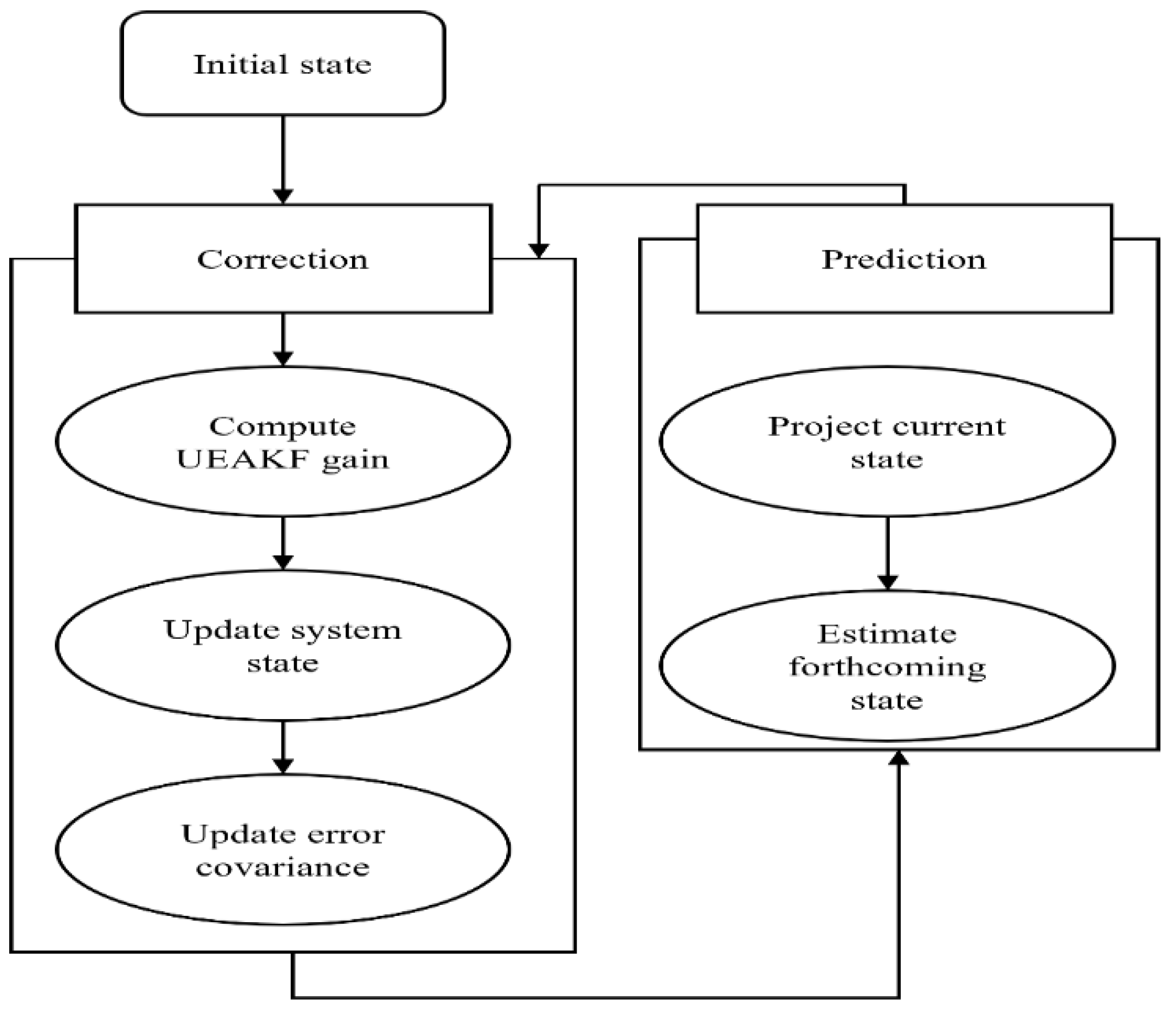
2.3. Prediction Phase

Suppose that the initial phase, $x_0\sim \mathcal{O}\left({\widehat{x}}_0,D_0\right)$ with ${\widehat{x}}_0$ and $D_0$ are known in advance. Since ${\alpha }_l^x$ and $y_l$ are uncorrelated, the state prediction ${\widehat{x}}_{l+1\left|l\right.}=F_l\left\{x_{l+1}\right\}$ becomes

$${\widehat{x}}_{l+1\left|l\right.}=O{\widehat{x}}_{l\left|l\right.}.$$

(23)

Because of the state-dependent noise, the estimator must take more care in measuring the error covariance matrix. We consider$X_l=X_l\left\{V\left(\left|x_l\right|\right)\right\}$. Given the tracking environment considered in Equation (20), the covariance of the corresponding presponding predictive model is ${\widehat{x}}_{l+1\left|l\right.}=F_l\left\{x_{l+1}\right\}$

$$D_{l+1\left|l\right.}=O{D}_{l\left|l\right.}{O}^R+G_l,$$

(24)

$$G_l=\delta {\delta }^R+{\delta }_x{\delta }_x^R+{\overline{\delta }}_{x}V\left(D_{l\left|l\right.}+{\widehat{x}}_{l\left|l\right.}+{\widehat{x}}_{l\left|l\right.}{\widehat{x}}_{l\left|l\right.}^R\right){\overline{\delta }}_x^R$$

(25)

2.4. Updation Phase

The estimate of the update phase ${\widehat{y}}_{l+1\left|l+1\right.}$ for the standard Kalman filter is described by the following equation.

$$\underset{y}{\min }\left(\Vert x-{\widehat{x}}_{l+1\left|l\right.}\Vert {}^2+\Vert z_{l+1}-I_x\Vert {}_{C^{-1}}^2\right)$$

(26)

where $C=w{w}^R\succ 0$. To make Equation (26) meaningful in Equation (25), in this work $G_l\succ 0$ is considered; thus, the predicted estimate is obtained from the following equation.

$${\widehat{x}}_{l+1\left|l+1\right.}={\widehat{x}}_{l+1\left|l\right.}+w^{*}$$

(27)

where $w^{*}$ represents the argument of the improved estimation model described by the following equation.

$$w^{*}=\underset{w}{\arg \min }\left({||w||}_{D_{l+1\left|l+1\right.}^{-1}}^2+\Vert a_{l+1}-L_w\Vert {}_{C^{-1}}^2\right),$$

(28)

where $w$ describes the estimated variance calculated using the following equation.

$$w=x-{\widehat{x}}_{l+1\left|l\right.}$$

(29)

and $e_{l+1}$ is an improved estimation model, determined by the following equation.

$$e_{l+1}=x_{l+1}-L{\widehat{x}}_{l+1\left|l\right.}$$

(30)

By modeling uncertainties and errors, we obtain a better estimator, as described below.

$$w^{*}=\underset{w}{\arg \min }F\left\{{||w||}_{D_{l+1\left|l+1\right.}^{-1}}^2+\Vert e_{l+1}-L_w+\left({\delta }_w+{\overline{\delta }}_{w}V\left(\left|w\right|\right)\right){\alpha }_{l+1}^w\Vert {}_{C^{-1}}^2\right\},$$

(31)

Here, ${\delta }_w,{\overline{\delta }}_w$ are new parameters added to the modified KF measurement model and ${\alpha }_{l+1}^w~\mathcal{O}\left(0,J\right)$ defines the noise added to the model. Thus, the improved update model results from the following equation.

$${\widehat{x}}_{l+1\left|l+1\right.}={\widehat{x}}_{l+1}+Q_{l+1}\left(z_{l+1}-L{\widehat{x}}_{l+1\left|l\right.}\right)-M_{l+1}{\gamma }_{l+1}$$

(32)

with

$$M_{l+1}={\left[J-\omega +\omega N_{l=1}\right]}^{-1}\omega ,$$

(33)

$$Q_{l+1}=Q_{l+1}{L}^R{C}^{-1},$$

(34)

$$N_{l=1}=D_{l+1\left|l\right.}^{-1}+\wedge \left(C^{-1}\right),$$

(35)

$${\gamma }_{l+1}=\frac{1}{2}\mathsf{\Delta }\left(C^{-1}\right)S\left(w^{*}\right).$$

(36)

2.5. Covariance Matrix

Equation (27) defines the modified updation equation through measuring noise variance impacting measurement update. However, to obtain the covariance matrix of Equation (27), it must satisfy the following constraint.

$$\begin{gathered} D_{l+1\left|l\right.}-Q_{l+1}\left[{\overline{\delta }}_{z}V\left(D_{l+1\left|l+1\right.}\right){\overline{\delta }}_z^R+{\delta }_z{X}_{l+1}{\overline{\delta }}_z+{\overline{\delta }}_z{X}_{l+1}{\delta }_z\right]Q_{l+1}^R \\ =\left(J-Q_{l+1}L\right)D_{l+1\left|l\right.}{\left(J-Q_{l+1}L\right)}^R+Q_{l+1}{\tilde{C}}_{l+1}{Q}_{l+1}^R+{\beta }_{l+1}{\mu }_l{\beta }_{l+1}^R, \end{gathered}$$

(37)

with

$${\tilde{C}}_{l+1}=w{w}^R+{\delta }_z{\delta }_z^R+{\overline{\delta }}_z\left({\widehat{x}}_{l+1\left|l+1\right.}{\widehat{x}}_{l+1\left|l+1\right.}^R\right){\overline{\delta }}_z^R,$$

(38)

$${\beta }_{l+1}=\left[M_{l+1}\left(J-Q_{l+1}L\right)\right],$$

(39)

$${\mu }_{l+1}=\left[\begin{array}{cc}{\gamma }_{l+1}{\gamma }_{l+1}^R& {\gamma }_{l+1}{n}_{l+1}^R\\ n_{l+1}^R{\gamma }_{l+1}^R& 0\end{array}\right],$$

(40)

$$n_{l+1}=O\left(\left(J-Q_{l}L\right)n_l+M_l{\gamma }_l\right).$$

(41)

The proposed modified Kalman filter in Equations (20), (24), (32) and (37) for UAV tracking is modeled with an updated parameter ${\delta }_w={\delta }_z$, ${\overline{\delta }}_w={\overline{\delta }}_z$, and run together with other existing Kalman filter-based tracking models. The performance of the proposed and the existing UAV tracking model, namely DMK, is measured using the RMSE by simulation in a nonlinear and noisy environment. The KFUEA algorithm achieves excellent tracking performance compared to state-of-the-art KF-based UAV tracking models, which have been experimentally demonstrated.

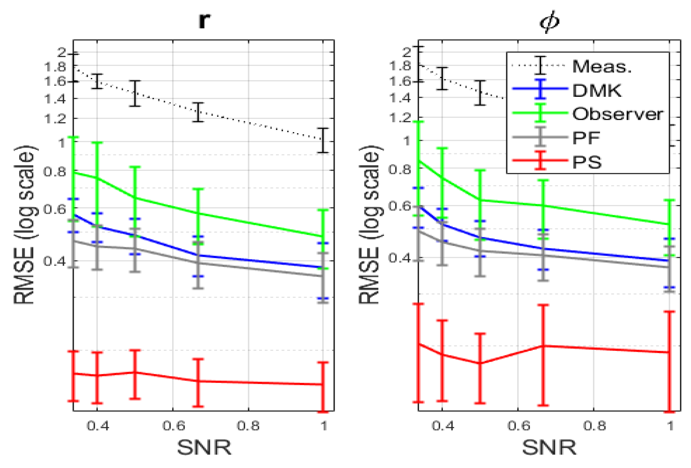
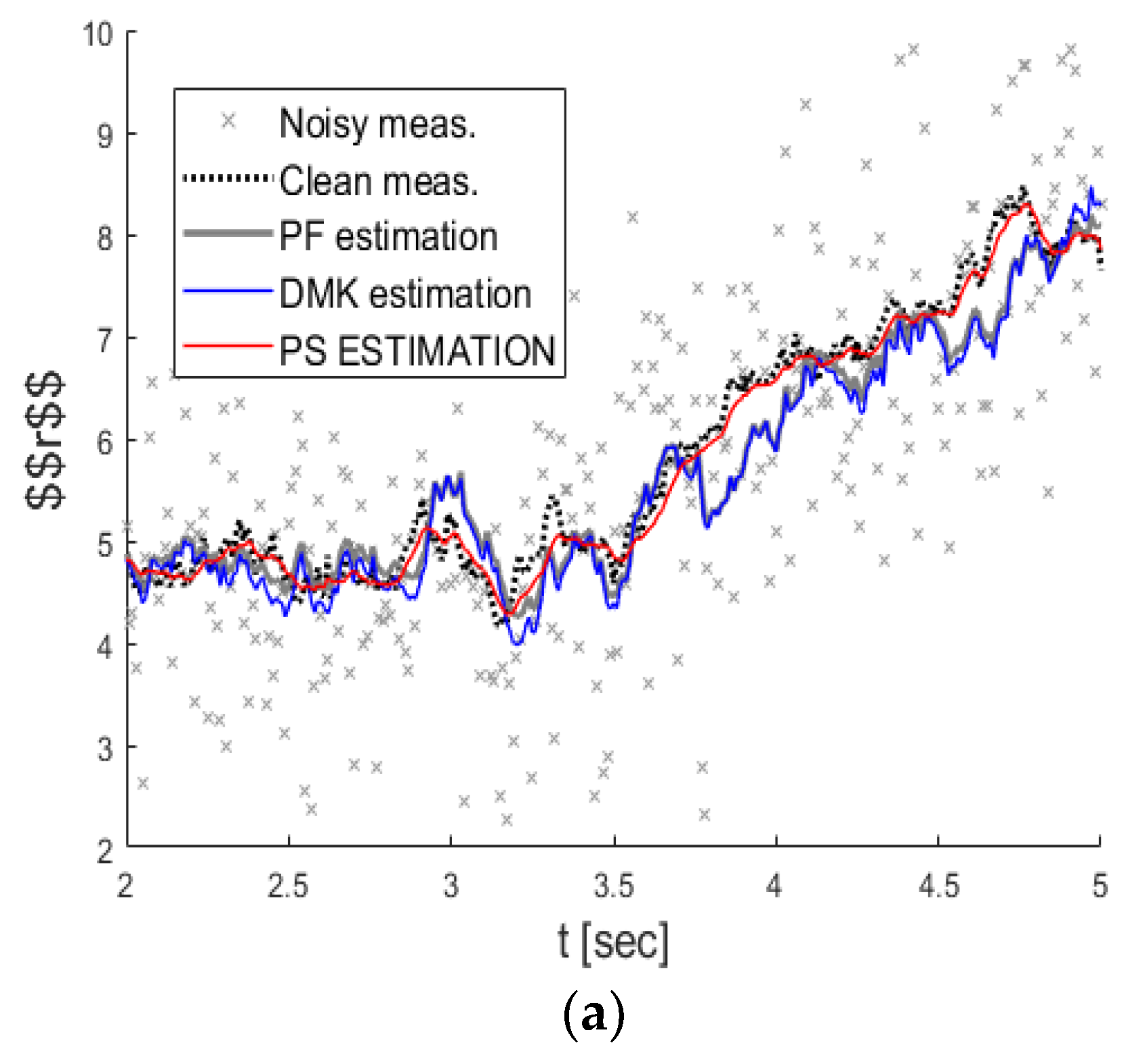
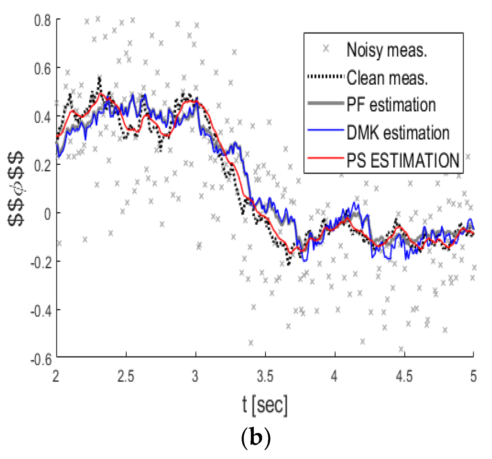
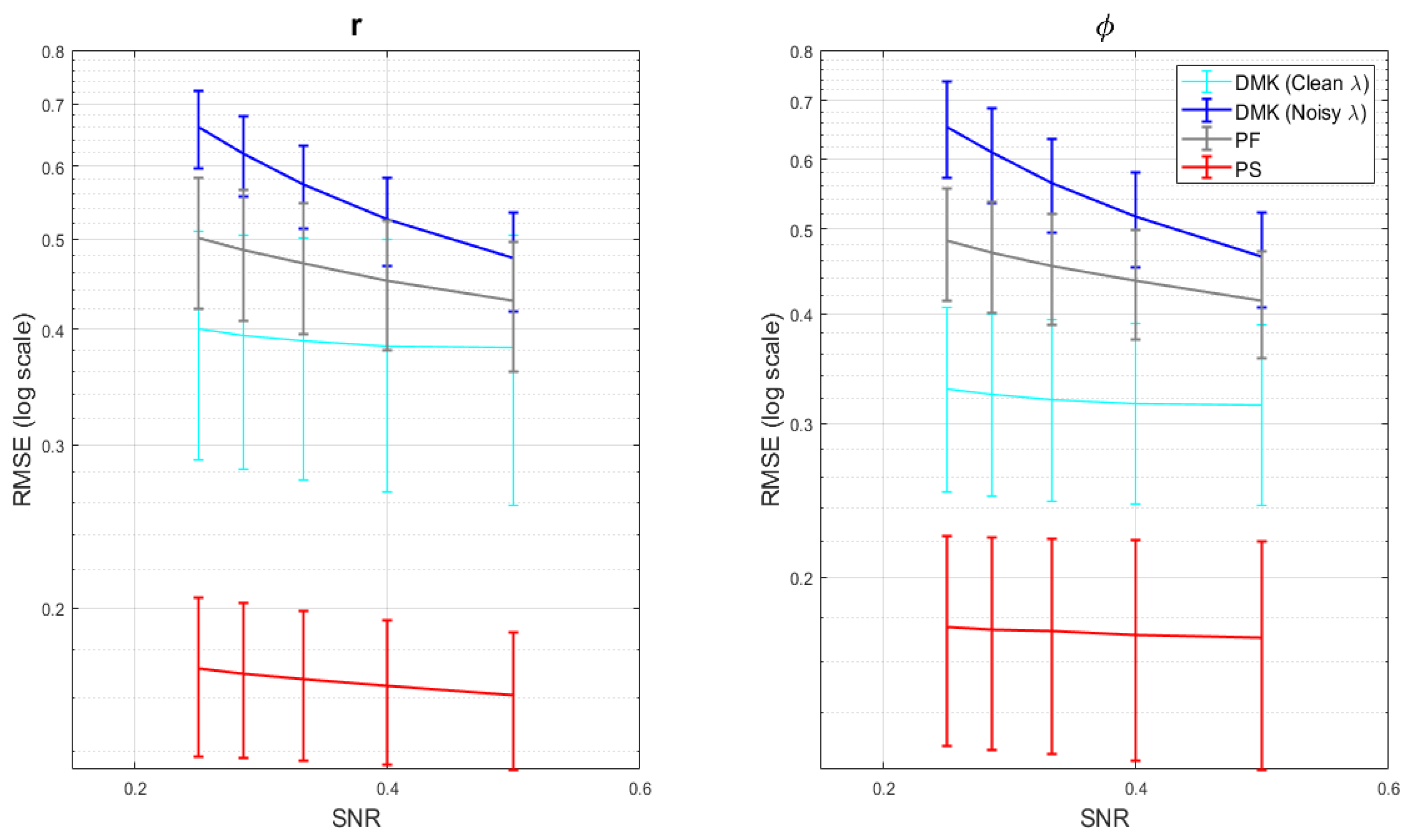
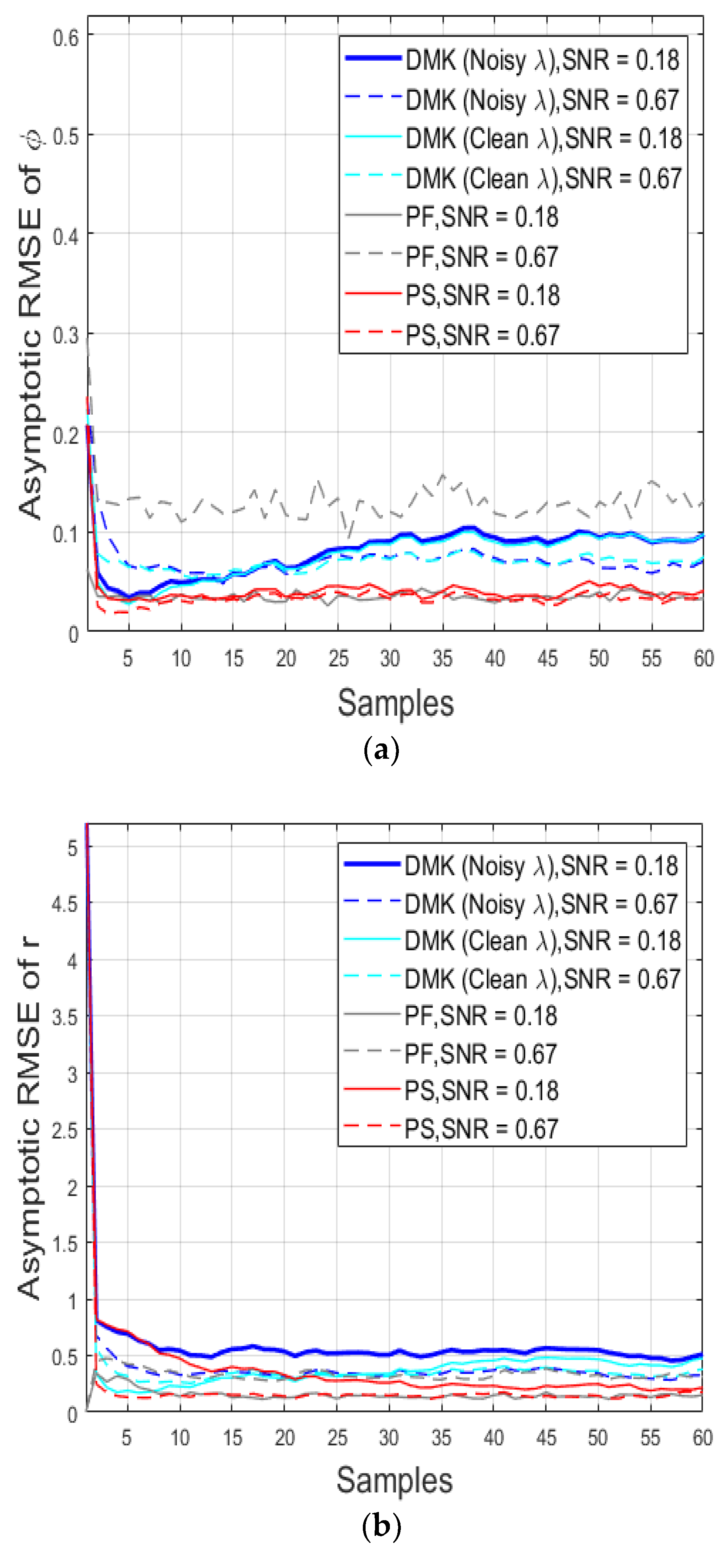
3. Simulation Analysis and Result

Here, an experiment is conducted to evaluate the performance of UAV tracking with the proposed KFUEA compared to various existing methods such as particle filter (PF) [40] and diffusion maps Kalman (DMK) [36] in a nonlinear environment with measurement functions and system dynamics. The experiment shows that KFUEA provides better state estimation compared to existing PF and DMK-based UAV tracking approaches.

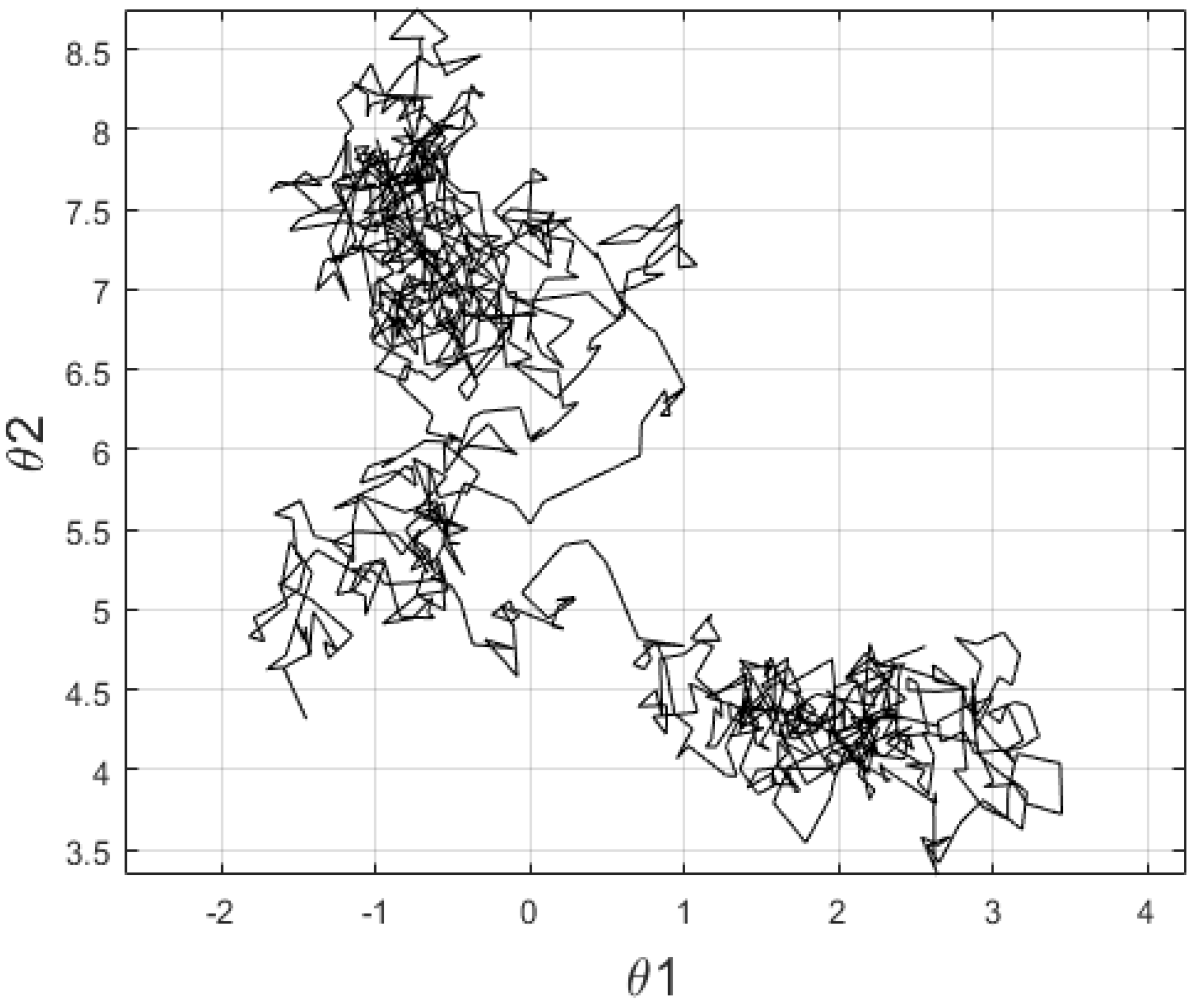
Nonlinear UAV Tracking Environment

Here we present a nonlinear tracking environment where the position of UAV considering two-dimensional (2D) space is measured using two parameters such as radius and azimuth angle. A sample 2D process obtained of uncertainty maneuvering of UAV is shown in Figure 3. The corresponding operation, which represents the Cartesian position of the UAV at different intervals, is represented as a discrete-time Langevin equation as follows.

$$\Delta {\theta }_{n+1}^{\left(1\right)}=-\frac{1}{2}{\left({\theta }_n^{\left(1\right)}-1\right)}^3+\left({\theta }_n^{\left(1\right)}-1\right)+\sqrt{2}{u}_n^{\left(1\right)}$$

(42)

$$\Delta {\theta }_{n+1}^{\left(2\right)}=-\frac{1}{2}{\left({\theta }_n^{\left(2\right)}-6\right)}^3+\left({\theta }_n^{\left(2\right)}-6\right)+\sqrt{2}{u}_n^{\left(2\right)}$$

(43)

Here, ${\theta }_n^{\left(1\right)}$ and ${\theta }_n^{\left(2\right)}$ represent Gaussian noise, and the drift terms define the double-well potentials. The UAV positions are calculated in polar coordinates using radius and azimuth as follows.

$${\varnothing }_n=arctan\left(\frac{{\theta }_n^{\left(1\right)}}{{\theta }_n^{\left(2\right)}}\right),r_n=\sqrt{{\left({\theta }_n^{\left(1\right)}\right)}^2+{\left({\theta }_n^{\left(1\right)}\right)}^2}$$

(44)

and the UAV tracking model measurement is generated by introducing Gaussian noise as follows.

$$Z_n=\left[{\varnothing }_n+v_n^{\left(\varnothing \right)},r_n+v_n^{\left(r\right)}\right],$$

(45)

where $v_n^{\left(\varnothing \right)}$ Gaussian noise with variance ${\sigma }_{\varnothing }^2$ and $v_n^{\left(r\right)}$ Gaussian noise operations with variance ${\sigma }_r^2$. Here, we generated 1000 samples of trajectories with the interval time of $\Delta t=0.01$ and varied the signal-to-noise ratio (SNR), by changing ${\sigma }_{\varnothing }^2$ and${\sigma }_r^2$. Then, KFUEA, PF, and DMK were applied simultaneously to evaluate the tracking performance of the different models for $z_n$.

Figure 4 shows the normalized root mean square error ($nRMSE$) results of the clean measurement estimation obtained by KFUEA and existing filtering methods such as PF and DMK. The $nRMSE$ is measured on a logarithmic scale; the ${\varnothing }_n$ and $r_n$ obtained by the corresponding filtering algorithms and the measurement error ($Meas$) provide an upper limit. The $nRMSE$ outcomes are obtained by varying the SNR level, and the mean and standard deviation of the $nRMSE$are computed for 50 samples considering the different SNR individually. Figure 4 shows that KFUEA performs better than conventional filtering methods such as PF and DMK at different noise levels. For both low and high SNR values, KFUEA outperforms PF and DMK.

Figure 5 shows the KFUEA predicted clean measurement (in red), PF (in gray), DMK (in blue), clean (dashed in black), and noisy measurement (in gray “x”) with SNR value set to 1. Figure 5a shows the measurement of $r_n$ and Figure 5b shows the measurement of${\varnothing }_n$. However, we obtain all values from the radar, the azimuth angle, and the radius. The values will always be noisy, so we do not obtain accurate values. The gray poses are all the values going into the system as input, and the black values are the clean measure. Therefore, our job is to protect the black value because those gray poses are contaminated (attack values/noisy values). The closer to the black values we obtain, the better results we obtain in the system. From the results, we can see that the KFUEA estimation is close to the true value, while the estimates of DMK and PF vary so much due to errors presented in their models (higher noise).

For evaluating the filtering algorithm under the presence of noise experiment is conducted. The corresponding $nRMSE$ considering different SNR levels are shown in Figure 6, where the mean and standard deviation of respective $nRMSE$ is computed for 50 samples considering different SNR level individually. From experiment it is seen that DMK clean achieves much better performance when compared with PF. However, with the presence of noise in the measurement model, the DMK noise performs badly when compared with PF. Thus, it shows the DMK model is affected due by the presence of noise. On the other side, the KFUEA achieves much better $nRMSE$ when compared with DMK noise and PF; further, achieve much better performance when compared with DMK without the presence of noise in the measurement model. This proves the robustness of KFUEA for tracking UAV in uncertainty, dynamic, and noisy environments.

Figure 7 and Figure 8 show the mean asymptotic RMSE ($aRMSE$), which is measured using the following equations

$$aRMSE=\sqrt{\frac{1}{M}{{\displaystyle \sum }}_{k=1}^M\Vert {\widehat{z}}_n^{\left(k\right)}-{\zeta }_n^{\left(k\right)}\Vert {}^2}$$

(46)

where $M$ defines the number of noisy samples considered, ${\widehat{z}}_n^{\left(k\right)}$ the estimates measured with the filter, and ${\zeta }_n^{\left(k\right)}$ the clean measurement in the instance $n$ of sample $k$. Figure 7 shows the results of KFUEA (in red), DMK noisy (in blue), DMK clean (in cyan), and PF (in gray), considering two different SNR levels. Figure 7a shows the $aRMSE$ outcomes for measurement coordinate ${\varnothing }_n$ and Figure 7b shows the $aRMSE$ outcomes for measurement coordinate$r_n$. From the results obtained, it can be interpreted that the convergence rate of KFUEA is not significantly affected due to noise. KFUEA achieves a much better convergence rate compared to PF and DMK when different SNR levels are considered.

Figure 8 shows the $aRMSE$ outcome achieved by KFUEA (in red), DMK (in blue), and PF (in gray) considering two different SNR levels. Figure 8a,c were obtained at an SNR level of 0.67, and Figure 8b,d were obtained at an SNR level of 0.18. From the results, it can be concluded that KFUEA achieves a better convergence rate compared with PF and DMK at different SNR levels.

4. Conclusions

Tracking UAVs has become more important because they provide not only location-based services but also pose serious security threats and vulnerabilities. UAVs are inherently smaller, move at high speeds, and operate at low altitudes, so it is conceivable to track UAVs with fixed or mobile radars. This paper presents a model for tracking UAVs that is efficient considering the volatility of UAV trajectory in a highly dynamic and noisy environment. Previous methods used particle filters and Kalman filters with diffusion maps to track UAVs. We have generated 1000 samples of trajectories with an interval time of ∆t = 0.01 and varied the signal-to-noise ratio (SNR) by changing the standard deviation of phi and the radius. Then, we applied KFUEA and the state-of-the-art PF and DMF simultaneously to measure and evaluate the tracking performance of the different models.

In this paper, initially $x_{l+1}$ and $z_l$ are computed using a modified Kalman filter matrix, an environmental matrix, and a measurement matrix. Then phase prediction is performed. After phase prediction, the phase estimation is updated for the Kalman filter. Then tracking the path of the unmanned aerial vehicle using the computed$x_{l+1}$ and $z_l$, and the updated phase. The KFUEA employs regularized least squares (RLS) for minimizing measurement error and brings good tradeoffs among preceding estimate confidence and forthcoming measurement under a dynamic environment.

However, under high uncertainties, the existing models performed very poorly. In the experiments, DMK is found to perform slightly better than PF at low noise levels. However, at higher noise levels, DMK performance deteriorates, and RMSE is slightly lower compared to PF-based UAV tracking methods. Therefore, DMK-based tracking cannot be used in high-uncertainty environments. In contrast, the KFUEA-based tracking model achieves very good RMSE compared to PF-based and DMK-based UAV tracking methods at lower and higher SNR values. Thus, the KFUEA is efficient enough to deal with the uncertain behavior of UAVs.

The safety of drone tracking is not always guaranteed because different drones have different signatures, and some drones try to mimic the signatures of other drones to avoid tracking. Developing an effective mechanism for tracking and detecting drone signatures is critical to counter malicious drones.

References

1. Hassanalian, M.; Rice, D.; Abdelkefi, A. Evolution of space drones for planetary exploration: A review. Prog. Aerosp. Sci. 2018, 97, 61–105. [Google Scholar] [CrossRef]
2. Goldman Sachs Research. Drones Reporting for Work. 2017. Available online: http://www.goldmansachs.com/our-thinking/technology-driving-innovation/drones/ (accessed on 1 September 2020).
3. Federal Aviation Administration. FAA Aerospace Forecast, FY 2016–2036. 2016. Available online: https://www.faa.gov/data_research/aviation/aerospace_forecasts/media/FY2016-36_FAA_Aerospace_Forecast.pdf (accessed on 17 August 2022).
4. Wang, X.; Chowdhery, A.; Chiang, M. Skyeyes: Adaptive video streaming from UAVs. In Proceedings of the 3rd Workshop on Hot Topics in Wireless, New York, NY, USA, 3–7 October 2016; pp. 2–6. [Google Scholar]
5. Haijun, W.; Haitao, Z.; Jiao, Z.; Dongtang, M.; Jiaxun, L.; Jibo, W. Survey on Unmanned Aerial Vehicle Networks: A Cyber Physical System Perspective. IEEE Commun. Surv. Tutor. 2020, 22, 1027–1070. [Google Scholar] [CrossRef] [Green Version]
6. Jean-Paul, Y.; Hassan, N.; Ola, S.; Ali, C. Security analysis of drones systems: Attacks, limitations, and recommendations. Internet Things 2020, 11, 100218. [Google Scholar]
7. Pietro, B.; Domenico, S.; Luigi, A.G. Internet of Drones: A Survey on Communications, Technologies, Protocols, Architectures and Services. arXiv 2020, arXiv:2007.12611. [Google Scholar]
8. Naser, H.M.; Tarik, T.; Osama, A. Low-Altitude Unmanned Aerial Vehicles-Based Internet of Things Services: Comprehensive Survey and Future Perspectives. IEEE Internet Things J. 2016, 3, 899–922. [Google Scholar] [CrossRef]
9. Riham, A.; Amr, M.Y. Security privacy and safety aspects of civilian drones: A survey. ACM Trans. Cyber-Phys. Syst. 2016, 1, 7. [Google Scholar]
10. Ben, N.; Asaf, S.; Ryusuoke, M.; Yuval, E. SoK—Security and privacy in the age of drones: Threats challenges solution mechanisms and scientific gaps. arXiv 2019, arXiv:1903.05155. [Google Scholar]
11. Matthew, R.; Francesco, F.; Herve, B. Micro UAV crime prevention: Can we help Princess Leia? In Crime Prevention in the 21st Century; LeClerc, B., Savona, E., Eds.; Springer: Cham, Switzerland, 2017. [Google Scholar]
12. Tamir, E. Mobile Radar Optimized to Detect UAVs, Precision Guided Weapons. Defense Update. 2013. Available online: https://defense-update.com/20130208_mobile-radar-optimized-to-detect-uavs-precision-guided-weapons.html (accessed on 22 July 2022).
13. Zhang, D.X. Research on electromagnetic interference mechanism of main remote control data link of UAV. J. Microwave 2016, 32, 90–96. [Google Scholar]
14. Jiang, Z.J.; Cheng, X.G.; Peng, Y.Q. Research on UAV identification algorithm based on deeplearning. App. Elec. Technol. 2017, 43, 84–87. [Google Scholar]
15. Zhao, J.C.; Fu, X.R.; Yang, Z.K.; Xu, F.T. Radar-Assisted UAV Detection and Identification Based on 5G in the Internet of Things. Wirel. Commun. Mob. Comput. 2019, 2019, 2850263. [Google Scholar] [CrossRef] [Green Version]
16. Schreiber, E.; Heinzel, A.; Peichl, M.; Engel, M.; Wiesbeck, W. Advanced buried object detection by multichannel, UAV/drone carried synthetic aperture radar. In Proceedings of the 2019 13th European Conference on Antennas and Propagation, Krakow, Poland, 31 March–5 April 2019; pp. 1–5. [Google Scholar]
17. Dill, S.; Schreiber, E.; Engel, M.; Heinzel, A.; Peichl, M. A drone carried multichannel Synthetic Aperture Radar for advanced buried object detection. In Proceedings of the 2019 IEEE Radar Conference, Boston, MA, USA, 22–26 April 2019; pp. 1–6. [Google Scholar]
18. Zhu, L.Z.; Zhao, H.C.; Xu, H.L.; Lu, X.Y.; Chen, S.; Zhang, S.N. Classification of Ground Vehicles Based on Micro-Doppler Effect and Singular Value Decomposition. In Proceedings of the 2019 IEEE Radar Conference, Boston, MA, USA, 22–26 April 2019; pp. 1–6. [Google Scholar]
19. Harvey, A.C. Forecasting, Structural Time Series Models and the Kalman Filter; Cambridge University Press: Cambridge, UK, 1990. [Google Scholar]
20. Liu, Z.X.; Xie, W.X.; Wang, P. Tracking a target using a cubature Kalman filter versus unbiased converted measurements. In Proceedings of the 2012 IEEE 11th International Conference on Signal Processing, Beijing, China, 21–25 October 2012; pp. 2130–2133. [Google Scholar]
21. Zhang, X.C.; Guo, C.J. Cubature Kalman filters: Derivation and extension. Chin. Phys. B 2013, 22, 128401. [Google Scholar] [CrossRef]
22. Chen, V.C.; Li, F.; Ho, S.S.; Wechsler, H. Micro-Doppler effect in radar: Phenomenon, model, and simulation study. IEEE Trans. Aerosp. Electron. Syst. 2006, 42, 2–21. [Google Scholar] [CrossRef]
23. Bordonaro, S.; Willett, P.; Bar-Shalom, Y. Decorrelated unbiased converted measurement Kalman filter. IEEE Trans. Aerosp. Electron. Syst. 2014, 50, 1431–1444. [Google Scholar] [CrossRef]
24. Basso, G.F.; De Amorim, T.G.S.; Brito, A.V.; Nascimento, T.P. Kalman Filter with Dynamical Setting of Optimal Process Noise Covariance. IEEE Access 2017, 5, 8385–8393. [Google Scholar] [CrossRef]
25. Mezi’c, I. Spectral properties of dynamical systems, model reduction and decompositions. Nonlin. Dyn. 2005, 41, 309–325. [Google Scholar] [CrossRef]
26. Marko, B.; Ryan, M.; Igor, M. Applied koopmanism. Chaos Interdiscip. J. Nonlinear Sci. 2012, 22, 47510. [Google Scholar]
27. Amit, S.; Andrzej, B. Linear observer synthesis for nonlinear systems using koopman operator framework. IFAC Pap. Online 2016, 49, 716–723. [Google Scholar]
28. Williams, M.O.; Ioannis, G.K.; Clarence, W.R. A data-driven approximation of the koopman operator: Extending dynamic mode decomposition. J. Nonlinear Sci. 2015, 25, 1307–1346. [Google Scholar] [CrossRef]
29. Klus, S.; Peter, K.; Christof, S. On the numerical approximation of the perron-frobenius and koopman operator. J. Comput. Dyn. 2016, 3, 51. [Google Scholar]
30. Berry, T.; Dimitrios, G.; John, H. Nonparametric forecasting of low-dimensional dynamical systems. Phys. Rev. E 2015, 91, 32915. [Google Scholar] [CrossRef] [Green Version]
31. Berry, T.; John, H. Nonparametric uncertainty quantification for stochastic gradient flows. SIAM/ASA J. Uncertain. Quantif. 2015, 3, 484–508. [Google Scholar] [CrossRef] [Green Version]
32. Ronald, R.C.; Stephone, L. Diffusion maps. Appl. Comput. Harmon. Anal. 2006, 21, 5–30. [Google Scholar]
33. Franz, H.; Tyrus, B.; Timothy, S. Ensemble kalman filtering without a model. Phys. Rev. X 2016, 6, 11021. [Google Scholar]
34. Floris, T. Detecting strange attractors in fluid turbulence. In Dynamical Systems and Turbulence; Springer: Berlin/Heidelberg, Germany, 1981. [Google Scholar]
35. Giannakis, D. Data-driven spectral decomposition and forecasting of ergodic dynamical systems. Appl. Comput. Harmon. Anal. 2017, 47, 338–396. [Google Scholar] [CrossRef]
36. Shnitzer, T.; Talmon, R.; Slotine, J.-J. Diffusion Maps Kalman Filter for a Class of Systems with Gradient Flows. IEEE Trans. Signal Process. 2020, 68, 2739–2753. [Google Scholar] [CrossRef] [Green Version]
37. Coifman, R.R.; Kevrekidis, I.G.; Lafon, S.; Maggioni, M.; Nadler, B. Diffusion maps, reduction coordinates, and low dimensional representation of stochastic systems. Multiscale Model. Simul. 2008, 7, 842–864. [Google Scholar] [CrossRef] [Green Version]
38. Mahfouz, S.; Mourad-Chehade, F.; Honeine, P.; Farah, J.; Snoussi, H. Target Tracking Using Machine Learning and Kalman Filter in Wireless Sensor Networks. IEEE Sens. J. 2014, 14, 3715–3725. [Google Scholar] [CrossRef] [Green Version]
39. Yunfeng, L.; Jidong, S.; Hamid, R.K.; Xiaoming, L. A Filtering Algorithm for Maneuvering Target Tracking Based on Smoothing Spline Fitting. Abstr. Appl. Anal. 2014, 2014, 127643. [Google Scholar]
40. Papaiz, A.; Tonello, A.M. Azimuth and Elevation Dynamic Tracking of UAVs via 3-Axial ULA and Particle Filtering. Int. J. Aerosp. Eng. 2016, 2016, 7630950. [Google Scholar] [CrossRef]
Figure 1. UAVs/Drones communication.
Applsci 12 11313 g001
Figure 2. KFUEA Flow Diagram.
Applsci 12 11313 g002
Figure 3. A sample two-dimensional space of UAV path.
Applsci 12 11313 g003
Figure 4. The clean measurement estimations’ nRMSE mean and standard deviation. The result of the n R M S E were averaged over 50 samples of process and noise trajectories.
Applsci 12 11313 g004
Figure 5. The estimations of the clean measurement for different algorithms with an SNR value of 1. (a) shows the measurement of r n . (b) shows the measurement of   n .
Applsci 12 11313 g005aApplsci 12 11313 g005b
Figure 6. Standard deviation and Mean of n R M S E of clean measurement estimates; n R M S E result were averaged over 50 samples of process and noise trajectories. A n R M S E comparison among KFUEA (in red) with DMK clean (in cyan), DMK noisy (in blue), and PF (in gray).
Applsci 12 11313 g006
Figure 7. Asymptotic Root Mean Square Error ( a R M S E ), averaged considering 50 samples of the measurement’s estimations for different algorithm DMK noisy (in blue), DMK clean (in cyan), PF (in gray), and KFUEA (in red). (a) shows the a R M S E outcomes for measurement coordinate n . (b) shows the a R M S E outcomes for measurement coordinate   r n
Applsci 12 11313 g007
Figure 8. a R M S E , averaged considering 50 samples of the measurement’s estimations for a different algorithm such as DMK (in blue), the PF (in grey), and KFUEA (in red). The SNR level is fixed at 0.67 for cases (a,c), and the SNR level is fixed at 0.18 for cases (b,d). The plots (a,b) show the outcome of a R M S E achieved for measuring coordinates n and the plots (c,d) show the outcome of a R M S E achieved for measuring coordinates   r n .
Applsci 12 11313 g008aApplsci 12 11313 g008b