Article

Forecasting of PM2.5 Concentration in Beijing Using Hybrid Deep Learning Framework Based on Attention Mechanism

1
Faculty of Geomatics, Lanzhou Jiaotong University, Lanzhou 730070, China
2
Chinese Academy of Surveying and Mapping, Beijing 100830, China
3
National-Local Joint Engineering Research Center of Technologies and Applications for National Geographic State Monitoring, Lanzhou 730070, China
4
Gansu Provincial Engineering Laboratory for National Geographic State Monitoring, Lanzhou 730070, China
*
Author to whom correspondence should be addressed.
Appl. Sci. 2022, 12(21), 11155; https://doi.org/10.3390/app122111155
Submission received: 21 September 2022 / Revised: 26 October 2022 / Accepted: 2 November 2022 / Published: 3 November 2022

Abstract

:
Air pollution has become a critical factor affecting the health of human beings. Forecasting the trend of air pollutants will be of considerable help to public health, including improving early-warning systems. The article designs a novel hybrid deep learning framework FPHFA (FPHFA is the abbreviation of the title of this paper) for PM2.5 concentration forecasting is proposed, which learns spatially correlated features and long-term dependencies of time series data related to PM2.5. Owing to the complex nonlinear dynamic and spatial features of pollutant data, the FPHFFA model combines multi-channel one-dimensional convolutional neural networks, bi-directional long short-term memory neural networks, and attention mechanisms for the first time. Multi-channel 1D CNNs are applied to capture trend features between some sites and overall spatial characteristics of PM2.5 concentration, Bi LSTMs are used to learn the temporal correlation of PM2.5 concentration, and the attention mechanism is used to focus more effective information at different moments. We carried out experimental evaluations using the Beijing dataset, and the outcomes show that our proposed model can effectively handle PM2.5 concentration prediction with satisfactory accuracy. For the prediction task from 1 to 12 h, our proposed prediction model performs well. The FPHFA also achieves satisfactory results for prediction tasks from 13 to 96 h.

1. Introduction

Along with the expansion of cities and industrial progress, the problem of urban air pollution has gradually become significant, has seriously affected people’s healthy life [1], and has attracted widespread attention in recent years. Forecasting of air quality has a vital role in preventing air pollution and protecting the environment [2]. PM2.5 (particulate matter with a diameter of less than 2.5 μm) is an essential indicator of the degree of air pollution [3]. Forecasting the trend of PM2.5 concentration has been regarded as one of the most important issues in the task of air quality prediction.
According to the length of time to forecast PM2.5 concentration, PM2.5 prediction models can be classified into short-term prediction models and long-term prediction models [4]. Short-term forecasting is real-time forecasting, focusing on forecast accuracy and ensuring the safety of human activities in the short term by keeping the forecast period within 12 h [5]. The purpose of long-term forecasting is to forecast PM2.5 concentration more than two days into the future [6], which can serve as a helpful reference for managers.
According to the research methods of PM2.5 prediction models, PM2.5 prediction models can be split into chemical transport models and statistical models. To achieve the purpose of pollutant concentration forecasting, the chemical transport model focuses on the mechanism of haze formation and the transport and dispersion process of pollutants. Representative chemical transport models can be found in the Community Multiscale Air Quality Modeling System (CMAQ) [7], the Nested Air Quality Prediction Modeling System (NAQPMS) [8], and the Weather Research and Forecasting Model with Chemistry (WRF-Chem) [9]. Although chemical transport models comprehensively consider the physical and chemical processes affecting the change of atmospheric pollutant concentration, their input data, such as emission sources and meteorological fields, are uncertain, and the models are computationally intensive and take a long time to compute [10]. Compared with chemical transport models, the approach of the statistical model is simple, efficient, and widely applicable. It learns and analyzes historical data, explores the intrinsic characteristics of the data, and gives more reasonable forecasting for the future based on the current state.
There are two main types of statistical models: machine learning and deep learning [11]. Machine learning mainly relies on regression forecasting in statistics, combining trends in air quality and other influencing factors to achieve PM2.5 concentration. Common models available for PM2.5 concentration prediction include random forest (RF) models [12], autoregressive moving average (ARMA) models [13], support vector regression (SVR) [14], and linear regression (LR) models [15]. Changes in PM2.5 concentration are strongly impacted by multiple factors like weather, traffic, and pollution sources, but the simple structure of machine learning models and the weak level of generalization of the models make it difficult to accurately represent the nonlinear, non-smooth process of PM2.5 changes. Compared to traditional machine learning models, deep learning models have also been adopted in the area of PM2.5 concentration forecasting due to their ability to obtain a more robust nonlinear fit to the data by a deeper number of hidden layers and effective training with a large volume of data.
Deep learning has demonstrated improved performance in temporal prediction to date, particularly in image identification [16], natural language processing (NLP) [17], the electricity sector [18], and prediction using historical data [19] (including the field of air pollutant concentration prediction). Deep learning models include convolutional neural networks (CNN) [20], backpropagation neural networks (BPNN) [21], recurrent neural networks (RNN) [22], gated recurrent units (GRU) [23], long short-term memory neural networks (LSTM) [24], and bidirectional long short-term memory neural networks (Bi LSTM) [25], which have been applied to forecasting of PM2.5 concentration. However, the prediction performance of the above deep learning models has improved to some extent. However, when the problem becomes complex, the prediction accuracy may be limited by the structure of a single network model. [26]. The hybrid deep learning model has several different network structures to better quantify complex data and create a better fit for changes in PM2.5 concentration.
Common hybrid deep learning models include LSTM fully-connected networks (LSTM-FC) [27], CNN-LSTM [28], attention-based CNN-LSTM (AC-LSTM) [29], and EEMD-GRNN model [30]. The above model forecasts PM2.5 concentration based on relevant historical data, such as pollutant data (e.g., PM10, SO2, CO) and meteorological data (e.g., dew point temperature, air pressure, wind direction). Moreover, PM2.5 concentration is a diffusion problem with spatial correlation. [31]. However, most studies focus on forecasting air quality at a single station with its historical data rather than the prediction of spatial correlation in neighboring regions. Consequently, the above model has three major issues. Firstly, it is challenging for the above model to thoroughly extract the spatial characteristics of the pollutant data, which makes it vulnerable to issues with feature information loss and decreased model predictive power. Secondly, it is difficult to extract the geographical and temporal correlation aspects of meteorological and pollutant data between several stations using the above approach. Finally, it is hard to extract the pollutant data’s long-term dependency due to the above model’s simplistic structure. To solve the above problem, we construct a hybrid deep learning model (FPHFA) based on the attention mechanism. The reasons are as follows.
(1)
Our model uses multi-channel 1D CNNs to process data from neighboring sites (i.e., pollutant data and meteorological data) to predict pollutant concentrations at the target site. This fully extracts the spatial characteristics among the stations and captures the spatiotemporal characteristics of the pollutant data and meteorological data.
(2)
The attention mechanism, as a lightweight module, does not consume too many resources of the computer. The attention mechanism matches the corresponding weights to the time series at different moments and concentrates the information that is more effective for prediction at different moments, thus improving the final prediction results.
(3)
Bi LSTM, as the prediction output layer, is more suitable for processing long time series spatiotemporal big data. Bi LSTM effectively utilizes the input forward and backward feature information to fully capture the long time series variation pattern of pollutant concentration.
In this paper, in order to make more accurate predictions of future PM2.5 concentrations in the target city, the following objectives should be achieved. (1) Efficient use of historical pollutant data and meteorological data from sites within the city; (2) In-depth extraction of spatial characteristics between sites; (3) Accurate realization of long-term prediction of pollutant concentrations at target sites.
The remainder of the piece is organized as follows. The pollutant concentration prediction model’s overall structure is described in Section 2, along with a thorough description of each component of the model. In Section 3 of the paper, the research area, the empirical data, and the methods for processing the experimental data are all given. The experimental findings from the experimental analysis are presented in Section 4. The experimental findings are given in Section 5, along with a discussion. The study’s work is summed up in the concluding part, along with potential topics for further investigation.

2. Research Method

2.1. Spatiotemporal Analysis

From the temporal dimension, the temporal characteristics of PM2.5 concentration on a monthly and seasonal basis are analyzed. From the spatial dimension, Kriging interpolation is applied to investigate the spatial distribution features of PM2.5 concentration. Kriging interpolation allows prediction of the value of a point to be measured by weighting the surrounding observations. The expressions are as follows.
Y ( m 0 ) = i = 1 n λ i Y ( m i )
Here Y ( m 0 ) is the interpolated value of the pointed m 0 to be estimated, Y ( m i ) is the feature of the measured point at position m i , n is the amount of measured data, and λ i is weighting factor. In Kriging interpolation, the weights λ i depend on the fitted model of the spatial relationship between the measured points in the model and the points to be estimated.

2.2. FPHFA Model

Figure 1 shows the framework of FPHFA and its components. The FPHFA framework is a clever mixture of multi-channel 1D CNNs, Bi LSTM, and the attention mechanism. To exploit the spatiotemporal correlation features of PM2.5-related time series data, the first task is to train multi-channel 1D CNNs to capture overall spatial characteristics of PM2.5 time series data from multiple stations.
Subsequently, the trend features between some sites and overall spatial characteristics extracted from the data from each site by the multi-channel 1D CNNs are connected using a concatenated layer and fed into the Bi LSTM. The Bi LSTM layer learns spatiotemporally dependent features from past and future contexts using both backward- and forward-oriented time series.
Then, we embed an attention layer between the two layers of the Bi LSTM. The attention-based layer weights the feature states at different times in the past and future and feeds the results to the second layer of the Bi LSTM to extract and learn the time-dependent features of the time series more accurately. The attention mechanism is the most important part of the FPHFA model, and it directly determines the prediction results. Finally, with the merged spatial characteristics, we input them into the fully connected layer for final prediction. Next, we will individually provide a detailed explanation of the detailed roles of the components of the FPHFA model individually.

2.2.1. Multi-Channel 1D CNNs for Learning of Overall Spatial Features

CNNs have excellent performance in grid-data processing and are widely used for image processing [32], while they can also be effectively applied to time series data analysis [20]. Here we use multi-channel 1D CNNs to process air quality time series data, assuming a given input model of L = [ l 1 , l 2 , , l t ] , including pollutant and meteorological data, are fed into the 1D CNN layer. The formula for the calculation process is as follows:
x t = tanh ( l t k t + b l )
where ∗ denotes the convolution operator, k t denotes the convolution kernel, b l denotes the bias vector, l t denotes the input vector, and x t denotes the output vector. The output of the 1D CNN layer is the spatiotemporal feature matrix, X = [ x 1 , x 2 , , x t ] . We use two convolutional layers for learning local trend characteristics. In the FPHFA model, we handle multi-site input time series data of air quality by multi-channel 1D CNNs, and the spatial features after convolution are given as feeds to the Bi LSTM layer through the concatenated layer.

2.2.2. Bi LSTM for Long-Term Series Learning

To overcome the problem of gradient reduction or gradient explosion, the LSTM is designed with a special cell storage structure. There are three gate structures for each LSTM cell structure, namely, the input gate, the output gate, and the forget gate. The specific derivation of the LSTM layer is as follows.
f t = σ ( W f [ h t 1 ,   x t ] + b f )
i t = σ ( W i [ h t 1 ,   x t ] + b i )
C ˜ t = tanh ( W C [ h t 1 ,   x t ] + b C )
C t = f t C t 1 + i t C ˜ t
O t = σ ( W o [ h t 1 , x t   ] + b o )
h t = O t tanh ( C t )
Here W f , W i , W C , and W o are the input weights, b f , b i , b c and b o are the deviation weights, t is the time state at the moment, t 1 is the last time condition, x t is the input vector, and h t is the output vector. The forget gate, f t , determines which data from the cell state should be deleted. The input gate, i t , determines what new data should be logged in the cell state. C ˜ t is a neuron with a self-recurrent cell like an RNN. C t is the internal storage unit of the LSTM block. The feature matrix H = [ h 1 , h 2 , , h t ] is the LSTM layer’s output.
LSTM has the limitation that it can perform work with previous content but cannot use predictions from future data. Schuster and Paliwal [33] introduced the idea of the bidirectional regression neural network (BRNN), which was combined with the LSTM to form the Bi LSTM. It has two distinct hidden LSTM layers with contrasting output directions. With this structure, the output layer can make use of both past and future information.
f t = σ ( W f [ h t 1 ,   x t ] + b f )
i t = σ ( W i [ h t 1 ,   x t ] + b i )
C ˜ t = tanh ( W C [ h t 1 ,   x t ] + b C )
C t = f t C t 1 + i t C ˜ t
O t = σ ( W o [ h t 1 , x t   ] + b o )
h t = O t tanh ( C t )
f t = σ ( W f [ h t 1 ,   x t ] + b f )
i t = σ ( W i [ h t 1 ,   x t ] + b i )
C ˜ t = tanh ( W C [ h t 1 ,   x t ] + b C )
C t = f t C t 1 + i t C ˜ t
O t = σ ( W o [ h t 1 , x t   ] + b o )
h t = O t tanh ( C t )
h t = h t h t
The above formulas show the Bi LSTM layer function. The positive and negative directions of the process are each represented by a separate directional arrow. The variable h t is concatenated by h t and h t , which represents the final result of the Bi LSTM cell. Through the process described above, the Bi LSTM enables the acquisition of the characteristics of past and future time series data and generates prediction outputs based on past and future contexts.

2.2.3. Attention Mechanism

Inputs at each period in the time series have different effects on the output results, and setting the same weights for the inputs at each moment reduces the forecasting accuracy to some extent. The attention mechanism matches the corresponding weights to the inputs at different moments to capture the most important temporal components that affect PM2.5 concentration [34]. The advantage of the attention mechanism is obvious; learning knowledge for more effective feature information is actually a process of accelerated denoising. To improve the utilization of information from past and future states, we added an attention layer to two-layer Bi LSTM. The importance of different eigenstates in the past and future is ranked, where H = [ h 1 , h 2 , , h t ] is the eigenstate matrix of the attention layer.
u t = tanh ( W h h t + b h )
α t = exp ( u t T v ) t exp ( u t T v )
s = t α t h t
Here u t and v represent the projection vectors, α t is the weight of normalized attention of h t , and s denotes the output vector weighted by the attention layer. Based on the weight of each vector in the eigenstate matrix H , Equations (22) and (23) allow the normalized weights of each vector to be calculated. Equation (24) provides the weighted vectors, which enable the calculation of the importance of the eigenstates at different moments.

3. Experimental Analysis

3.1. Research Area

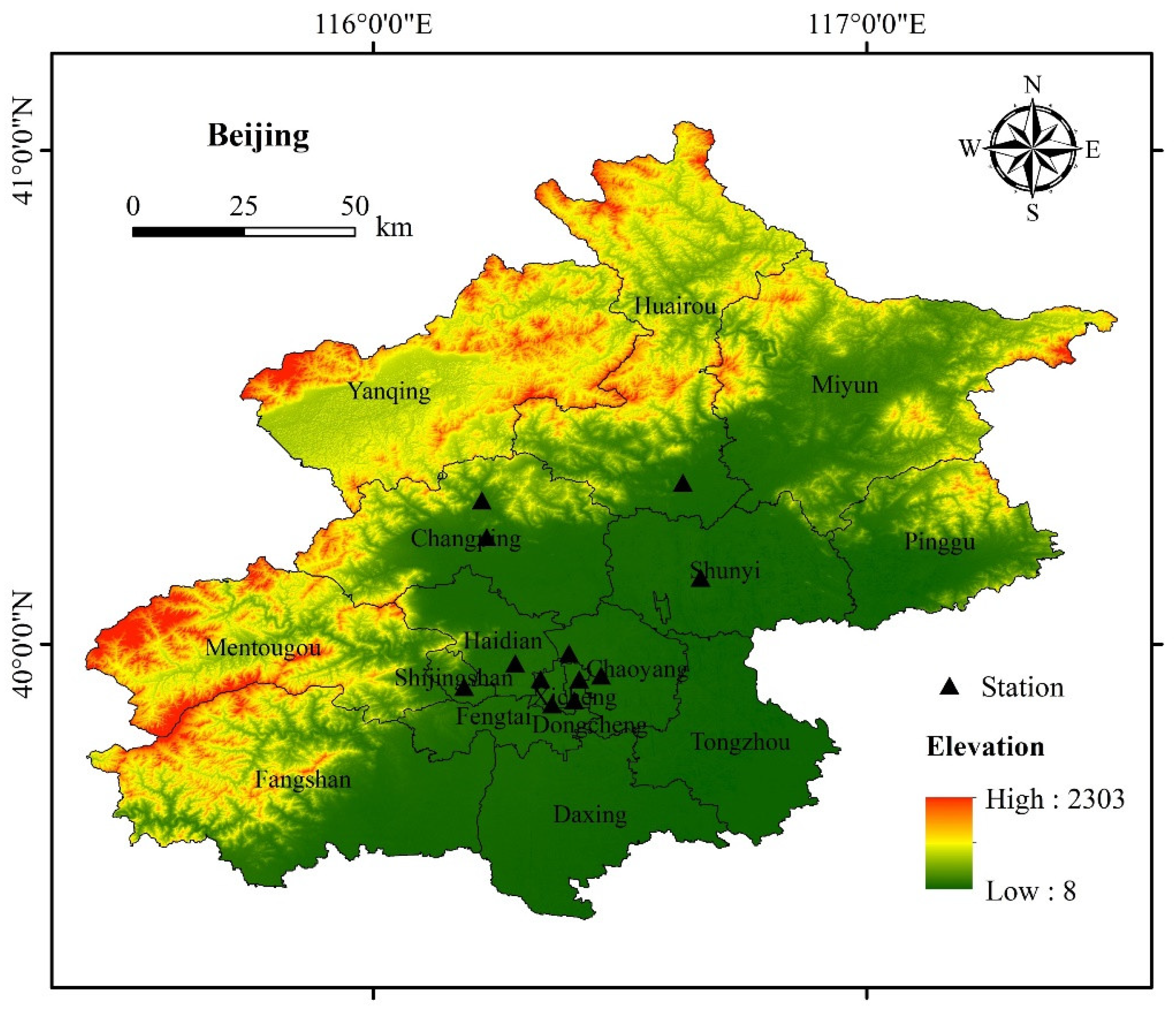
Beijing was chosen as the region of study because it is one of the most economically developed regions in China and also because it suffers from severe air pollution. The eastern part of Beijing borders Tianjin, a heavily industrial city, and the rest is bordered by Hebei Province. As shown in Figure 2, Beijing is bounded by the Taihang Mountains in the west, the Yanshan Mountains in the north, and a plain that slopes gently toward the Bohai Sea in the southeast. Beijing has four distinctive seasons, the summers are hot and rainy, with most of the annual precipitation concentrated in summer, and the winters are cold and dry. Due to the coupling of its particular geographical location, topographic features, and the coupling of climatic conditions, pollutants such as PM2.5 released from the heavy industrial areas around Beijing are difficult to disperse and, therefore, cause serious problems for the air quality of Beijing.

3.2. Data Description and Preprocessing

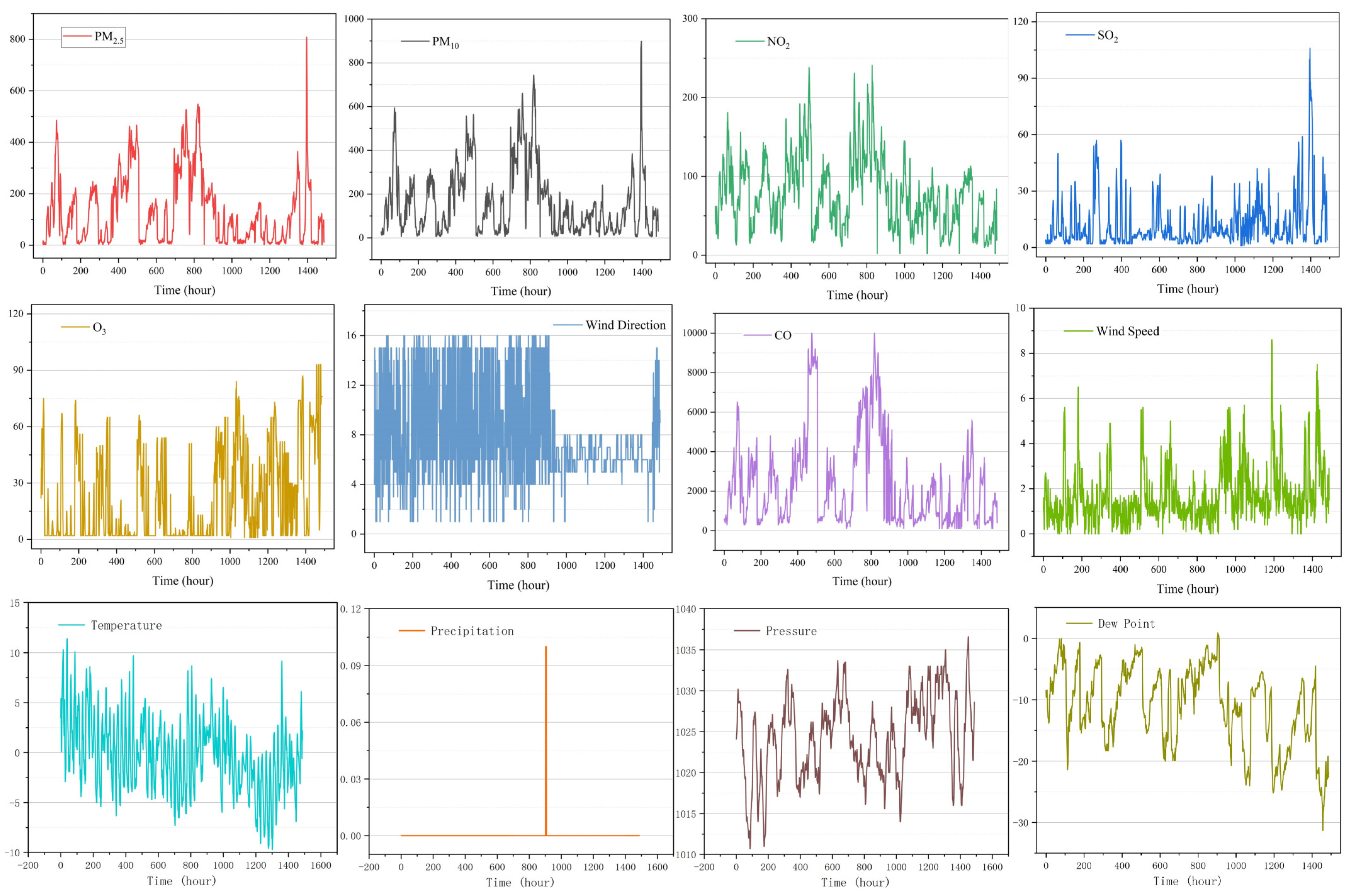
In this paper, hourly air quality concentration and meteorological data from twelve national ambient air pollutant monitoring stations during the period 1 March 2013 to 28 February 2017 were taken from the website of the University of California, Irvine (https://archive.ics.uci.edu/ml/datasets/Beijing+Multi-Site+Air-Quality+Data, accessed on 21 July 2022). The obtained air pollutant data (Table 1) include hourly PM2.5 and PM10. Hourly meteorological data obtained include temperature and pressure. The numerical changes of factors in Figure 3 are in the temporal dimension from 1 December 2016 to 31 January 2017.
In data preprocessing, firstly, as shown in Table 1, since wind direction is provided as non-numerical data, the wind direction type must be converted to numerical data for calculation using category coding. Secondly, the missing data for each site is less than 5%, thus preserving the data for all sites [26]. Missing values in the individual site data were estimated using linear interpolation from the previous and subsequent data points. Finally, to remove the influence of excessive differences in values on the accuracy of the model, all data are processed by the Min–Max function.

3.3. Experimental Setup

Comparative deep learning models and FPHFA models were built using TensorFlow. We utilized two layers of 1D CNN for learning local trends of features. Each layer was set to use the same filter size and kernel size, i.e., (62, 2), and ReLU was used as the activation function. We used two Bi LSTM layers for temporal feature learning with 128 hidden neurons per layer. The loss function of the FPHFA model is the mean squared error (MSE). Additionally, to prevent underfitting or overfitting of the model, The Beijing dataset was packaged and separated into a training set (80%) and a test set (20%).
In this article, we use root mean square error (RMSE), mean absolute error (MAE), correlation coefficient (R2), index of agreement (IA), and Mean Absolute Percentage Error (MAPE) to evaluate the performance of the prediction models. The calculation formulae are shown below.
RMSE = 1 n i = 1 n ( y i y ^ i ) 2
MAE = 1 n i = 1 n | y i y ^ i |
R 2 = i = 1 n ( y ^ i y ¯ i ) 2 i = 1 n ( y i y ¯ i ) 2
IA = 1 i = 1 m ( y i y ^ i ) 2 i = 1 n ( | y i y ¯ | + | y ^ i y ¯ | ) 2
MAPE = 1 n i = 1 n | y i y ^ i | y i
Here n is the number of samples, y i is the actual value of PM2.5, y ^ i denotes the corresponding predicted value, and y ¯ denotes the average of all PM2.5 values.

4. Results

4.1. Spatial and Temporal Features of PM2.5 Concentration

As shown in Figure 4, in different seasons and months, the PM2.5 concentration varied considerably. The PM2.5 concentration was low and stable in summer, higher in autumn and spring, and most severe in the winter. This is because the high temperature in summer can lead to atmospheric instability, triggering an increase in rainfall and high humidity, leading to large-scale wet deposition of suspended particles [35]. PM2.5 concentration was higher during spring than summer but showed a decreasing trend. In March, dry weather and high winds produced more soil dust, but air pollution eased as temperatures rose and rainfall increased in April and May. In autumn, seasonal factors such as weak winds, steady climate, and more frequent burning of biomass during harvest season [36] contributed to an increase in pollutants. In Beijing, the high PM2.5 concentration mainly occurred in winter, from November to February, with the peak occurring in December. The highest PM2.5 concentration in winter was mainly due to coal heating, burning of biomass, and fireworks during the Spring Festival, which has a great adverse effect on the atmospheric environment [37]. Furthermore, in winter, when the dry climate is unfavorable for air dispersion, suspended particles, organic or inorganic, could also lead to large amounts of pollutants in the air.
From the spatial dimension, the Kriging interpolation model was conducted for the average PM2.5 concentration at twelve sites in Beijing from 1 December 2016 to 31 December 2016 (the winter season with the highest PM2.5 concentration and the greatest variation). This indicated that the PM2.5 concentration of twelve stations in Beijing showed a clear spatial aggregation. As shown in Figure 5, PM2.5 concentration was higher in the southeastern part of Beijing and lower in the northwestern part, varying between 85 and 121 μg/m3. The areas with higher PM2.5 concentration were mainly concentrated in the main urban areas of Beijing, where the highest value is 121 μg/m3. As the main urban area of Beijing, southeastern Beijing was a transportation and scenic area as well as a mixed area with high emissions of vehicle exhaust, which led to high PM2.5 concentration [38,39]. As the distance from the central city increases, the PM2.5 concentration gradually decreases, and the atmospheric environment is improved (Figure 5). The areas with low PM2.5 concentrations are mainly concentrated in the countryside of Beijing, where the lowest PM2.5 concentration is 85 μg/m3. Generally speaking, for various reasons, PM2.5 concentration in Beijing shows a trend of gradually decreasing in the southeast to the northwest. The main reason was that Beijing was surrounded by mountains in the northwest, north, and northeast, and pollutants from the main urban area were blocked by the Taihang Mountains and Yanshan Mountains when they dispersed, resulting in large differences in the spatial distribution of PM2.5 concentration in Beijing [40] (In this study, data from 12 monitoring stations were used to fit the spatial variation of PM2.5 concentration in the entire Beijing region, resulting in incorrectly high PM2.5 concentration values in the northeast of Beijing. However, when we analyze the spatial variation of PM2.5 concentration, we choose to ignore it).
From this, it can be seen that PM2.5 is a series of data that changes with time, and PM2.5 has spatial variability and spatial correlation. Therefore, we specially design the FPHFA model to deal with PM2.5 data.

4.2. Analysis of Short-Term Prediction Results

LSTM, GRU, CNN-LSTM, and DAQFF (The model is proposed in the Deep Air Quality Forecasting Using Hybrid Deep Learning Framework text) are used as excellent models for processing time series data, and we use them as comparison models with the same model parameters set as FPHFA. Table 2 presents the short-term prediction quantitative results of the short-term prediction of PM2.5 from the Beijing dataset, which gives a comparison of LSTM, GRU, CNN-LSTM, DAQFF, and the FPHFA model in terms of RMSE, MAE, R2, and IA. From Table 2, we can see that the FPHFA model performs better than other deep learning models in the task of short-term PM2.5 concentration prediction for the Beijing dataset. In the Beijing dataset, FPHFA improves R2 to 0.877, IA to 97.04%, and MAPE to 0.561 while reducing RMSE to 28.15 and MAE to 19.19 compared to the other comparison models, which represents an obvious improvement in the accuracy of the prediction. Additionally, the classic deep learning models’ model performance evaluation indicators are comparable but inferior to those of the hybrid deep learning models. The implication is that hybrid deep learning models are superior to traditional deep learning models for short-term PM2.5 concentration prediction. Moreover, our model performs the best among hybrid deep learning models. Compared with the DAQFF model, FPHFA improved R2 by 0.018 and IA by 0.57% while reducing RMSE by 1.97 and MAE by 1.83. This is because FPHFA can learn local trend features through the unique multi-channel 1D CNNs, and long-term dependence of PM2.5 concentration can be obtained by Bi LSTM. Moreover, the additional most important attention mechanism effectively focuses on information that is more significant for prediction at particular moments, thus improving the final prediction results.
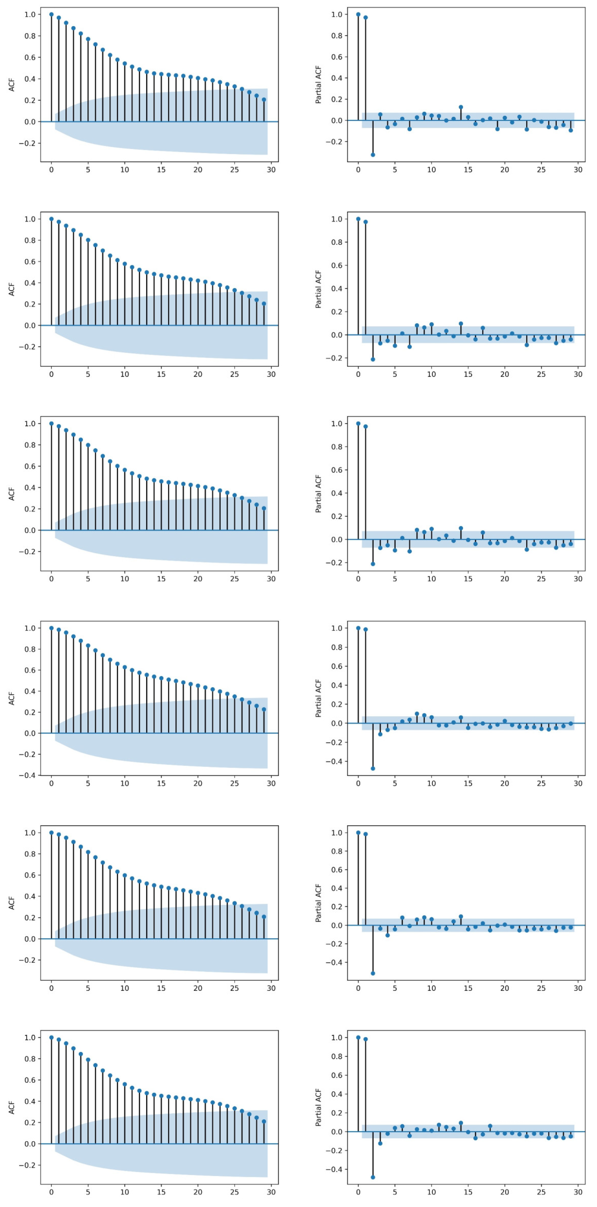
In order to clearly describe the prediction results of the model, examples of the Autocorrelation Function (ACF) and Partial Autocorrelation Function (PACF) are plotted in Figure 6. We use the predicted results of the model to make an example diagram. Compared with other models, the prediction results of our model also have a significant correlation. This shows that our model is superior to other models.
In addition, the selection of window size (representing the input size of the model’s historical observations) also has an impact on short-term prediction performance. We investigate the influence of the window size for the deep learning model in the Beijing dataset. As shown in Figure 7, when the window size is larger than 32, the FPHFA model outperforms the other models in prediction performance. This is due to the fact that when the window is too tiny, the historical data available for learning is insufficient, and the capacity to forecast is hampered by data from nearby sites, leading to inaccurate PM2.5 concentration predictions by the FPHFA model for the target station. The FPHFA’s performance evaluation indicators optimize as the window size increases, and the RMSE of FPHFA reaches its minimum value (and IA its maximum) when the window size is about 56. Beyond this point, the model performance evaluation indicators remain constant or slightly increase, which may be a sign that the prediction models are overfitting.
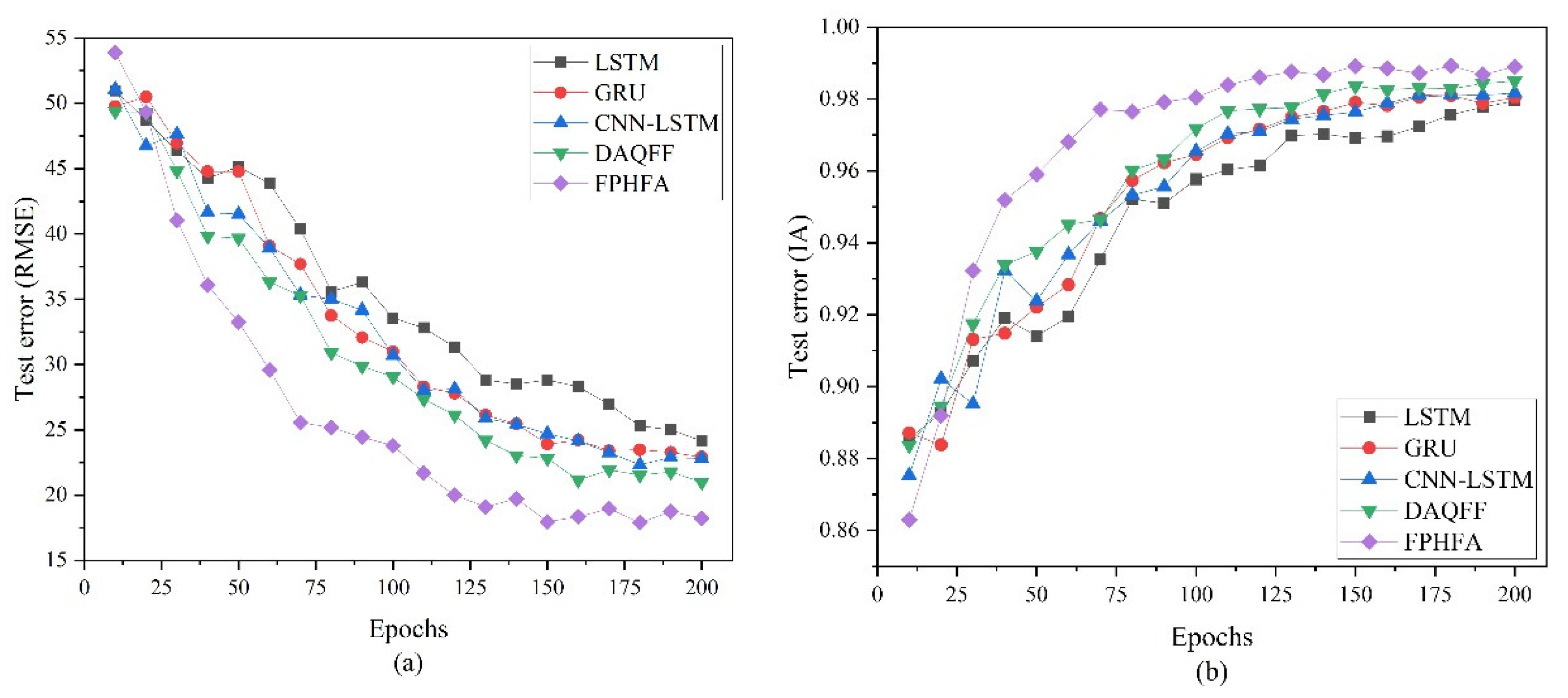
Next, we study the influence of the number of epochs on prediction performance by the different models. Figure 8 shows the model performance evaluation indicators (RMSE and IA) curves of the FPHFA relative to different epochs and provides comparisons with other prediction models. It is evident that FPHFA consistently outperforms the other deep learning models at almost any number of epochs. Moreover, the RMSE of FPHFA reaches its minimum (and the IA its maximum) when the number of epochs is about 150. This is followed by progressively unstable model performance as the epoch size keeps expanding. It is clear that as the number of epochs increases beyond 150, the generalization capacity does not. In addition, the optimization of all models seems to be a bit slow, and overfitting seems likely when the number of epochs exceeds 150. The more epochs there are, the more computational resources are used. On the other hand, as epochs increase, the training performance of the model may improve, but this can also lead to overfitting problems.
To further investigate the short-term prediction performance of models, we investigate the PM2.5 concentration forecasting ability of FPHFA and other deep learning models throughout the course of a month (744 observations in total). Figure 9 shows the comparison of the actual PM2.5 value with the value predicted 12 h ahead by the models LSTM, GRU, CNN-LSTM, DAQFF, and the proposed FPHFA model in the experiment with the Beijing dataset. As shown in Figure 9, compared to other deep learning models, the CNN-LSTM model has a lower match between the actual value and forecasted value. Beijing had the highest PM2.5 concentration in December, and the CNN-LSTM model may not be sensitive to such high values of PM2.5 concentration. It is obvious that the FPHFA outperforms LSTM, GRU, CNN-LSTM, and DAQFF in the task of 12-h forward prediction, especially as regards the time periods between the peaks and valleys of PM2.5 data. In addition, as shown in Figure 9, the prediction results of the FPHFA are highly similar to the observed results, while it also has a good fit at the points of sudden change in PM2.5 concentration.
In summary, compared to the short-term PM2.5 concentration prediction under different experiment conditions, the hybrid deep learning models’ forecasting performance is generally not poor, and FPHFA continues to have the greatest performance. Given how easy it is to anticipate time series in the near run, high prediction performance can frequently be obtained by simply following the trend of the preceding hours.

4.3. Analysis of Long-Term Prediction Result

In contrast to the foregoing short-term prediction task, long-term prediction is not so straightforward; it is often challenging to foresee what happens several days later. Next, we analyze the longer-term PM2.5 concentration prediction performance of the model. The quantitative results of long-term PM2.5 concentration prediction for the Beijing dataset are reported in Table 3, which provides a comparison of RMSE, MAE, R2, and IA from classical deep learning models, hybrid deep learning models, and the FPHFA model. Table 3 shows the FPHFA model outperformed other prediction models in long-term PM2.5 concentration prediction. Compared to other comparison models, the RMSE of FPHFA in the Beijing dataset is reduced to 22.12, MAE is reduced to 15.27, MAPE is reduced to 0.438, R2 is improved to 0.932, and IA is improved to 98.30%, which represents an obvious improvement in the accuracy of prediction. In addition, the error of the DAQFF model of hybrid deep learning models is inferior to that of the CNN-LSTM, but the difference between the two models is not large, and the error of both models is lower than that of the classical deep learning models. This implies that the hybrid deep learning approach is more suitable than the classical deep learning model for the task of predicting PM2.5 concentration prediction over the long term. Additionally, compared with the DAQFF model, FPHFA improved R2 by 0.068 and IA by 1.47% while reducing RMSE by 7.03 and MAE by 5.3. the results demonstrate that our FPHFA model performs better for both short-term and long-term prediction than DAQFF models.
The impact of prediction size on FPHFA and other deep-learning models is then examined. Figure 10 shows that as the forward prediction size increases, the performance of the prediction for those models gradually decreases. It is important to note that the model performance evaluation indicators of traditional deep learning models are comparable to and occasionally even superior to those of CNN-LSTM when the prediction size is smaller than 60. Does this imply that CNN-LSTM’s predicting performance is inferior to some traditional deep learning models? In fact, such is not generally the case, as Figure 10 also shows that the prediction performance of the hybrid deep learning models exceeds that of the classical deep learning models as the prediction horizon lengthens. Moreover, compared to models, the predicting performance of the LSTM, GRU, and CNN-LSTM models exhibits large fluctuations in long-term prediction at certain prediction horizons (e.g., 24–36 h, 72–84 h). The findings in Figure 10 are very noteworthy since they show that as the prediction size increases, FPHFA outperforms other models at any prediction time step (24–96 h) and is more stable. Moreover, we observe that compared with other models, FPHFA also has the lowest prediction error (RMSE and MAE) and the highest prediction accuracy (R2 and IA) at different prediction sizes.
In order to verify the prediction performance of the model in different periods, we divided the data into four groups according to seasons and used the model to predict the pollutant data in different seasons. Table 4 and Table 5 show the comparison of the five deep-learning models in different seasons. For the prediction of pollutant concentration in different seasons, the model we designed has achieved the optimal prediction results. In addition, it is obvious that the prediction accuracy of the model has some seasonal differences. In terms of reducing the prediction error and improving the consistency between the predicted data and the real data, the prediction results of the model in different seasons are not the same. In the spring and summer forecast, the forecast error is low, but the consistency between the predicted data and the real data is not high. In autumn and winter, larger forecast errors correspond to a higher agreement. Considering the seasonal characteristics of PM2.5 concentration, we found that the prediction error may be related to PM2.5 concentration and dispersion in different seasons. In summer, PM2.5 concentration is usually low, and the prediction error is small, but the consistency between the predicted value and the real value is not high. In winter, the concentration of PM2.5 is high, the dispersion is large, and the uncertainty of the variation of pollutant concentration is also high, which leads to the difficulty of pollutant prediction. High PM2.5 concentration limits the prediction ability of the deep learning model, leading to the largest prediction error in winter among all seasons [41]. This is also the reason why the PM2.5 concentration values in December 2016 and January 2017 were selected as the prediction criteria in this study.
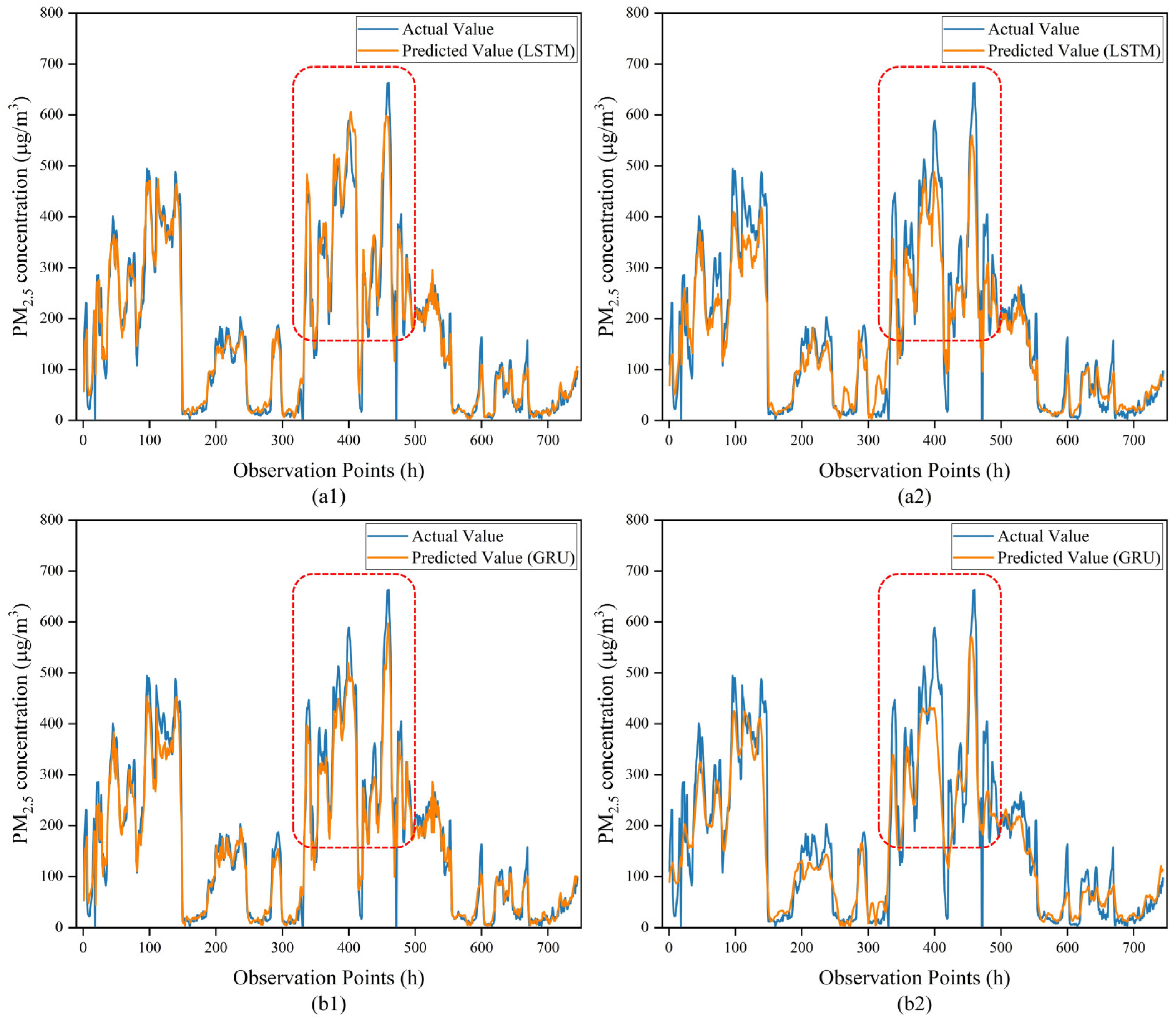
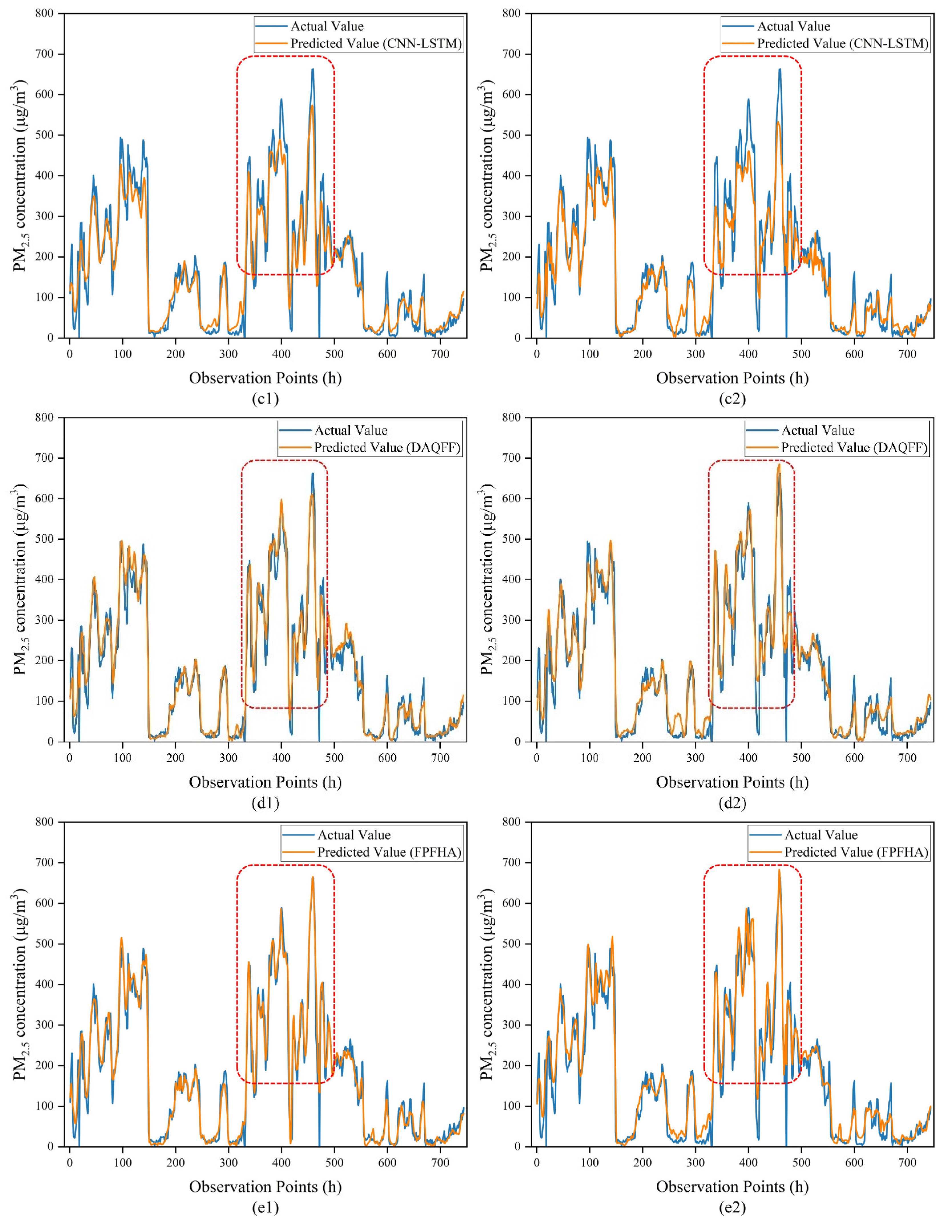
To evaluate the long-term prediction performance of FPHFA and other deep learning models on the Beijing dataset, we investigate the PM2.5 concentration forecasting capability of FPHFA and other deep learning models under different prediction sizes (24 h and 96 h) throughout the course of a month (744 observations in total). Comparing the actual and predicted PM2.5 values for several models (LSTM, GRU, CNN-LSTM, DAQFF, and FPHFA) at various time steps is shown in Figure 11 (24 h and 96 h). Figure 11 shows that the long-term predictive performance of FPHFA is superior to both classical deep learning models and other hybrid deep learning models at different time steps, especially with regard to the peak and valley periods of the test data. In addition, for prediction tasks, including sudden changes in pollutant concentration, FPHFA outperforms comparative models. Moreover, the FPHFA model consistently has the greatest prediction performance for long-term PM2.5 concentration predictions at any time step.
In order to further assess the model’s capacity for fitting data and confirm the claim that FPHFA can provide a more accurate representation of sudden change points, as shown in Figure 11 and Figure 12, when the concentration of PM2.5 is not stable, especially when the value is higher than 400, the outcomes of the compared model cannot follow the actual values, and the error is visibly larger. This reveals that it is challenging for the model to provide a reliable prediction of PM2.5 concentration for such horizon values. Furthermore, we find that in comparison to the other models, FPHFA can predict high PM2.5 concentrations with accuracy, giving a high consistency between predicted and observed values. In combination with the experimental outcomes in Figure 11 and Figure 12, we can clearly see that, in general, the mutation points of PM2.5 concentration appear at higher concentrations and in smaller numbers. This phenomenon causes the problem of inadequate learning of prediction models, and it is challenging for the models to learn the change patterns of PM2.5 concentration under sudden changes. This is why most deep learning models yield poor fits to the data in the presence of sudden changes in PM2.5 concentration.
In conclusion, for the proposed FPHFA, the long-term prediction efficacy is greater than for other deep learning models. The long-term predicted PM2.5 concentration of the FPHFA model is well matched with the actual values, which means that FPHFA can usefully study the spatial correlation and long-term time-dependent features of PM2.5 time series data.

5. Discussion

The results show that the performance of FPHFA is best among all models tested for short-and long-time PM2.5 forecasting. In comparison to other hybrid deep learning models and traditional deep learning models, the deep learning framework based on the attention mechanism becomes a more useful tool for handling spatiotemporal data.
In terms of the temporal dimension, there was a significant seasonal variation in PM2.5 concentrations, which show a declining sequence of winter, spring, autumn, and summer, with a U-shaped change on both seasonal and monthly scales. From the spatial dimension, PM2.5 concentration was higher in the southeastern part of Beijing, lower in the northwestern part of the city, and gradually declined from the heart of the city towards the countryside.
As a result of the experimental findings, the study shows that indicates that the FPHFA has the best prediction performance compared to other models for both short-term and long-term PM2.5 prediction. Compared to other models, FPHFA is more accurate in predicting the peaks and valleys of PM2.5 concentration at various time steps. In long-term PM2.5 concentration prediction, FPHFA still outperforms other models despite sudden changes in pollutant concentration. Meanwhile, FPHFA can predict high PM2.5 concentrations with accuracy, enabling a high consistency between predicted and observed values. After the experimental comparison with the DAQFF model, the outcomes revealed that FPHFA can learn long-term time-dependent features in PM2.5 concentration data. Our proposed model performs so well due to (1) multi-channel 1D CNNs fully extracting the spatial features between sites and the spatiotemporal features between historical data; (2) Bi LSTM fully extracting the changing features of pollutant data by using the information features in both directions; (3) the attention mechanism according to assigning different weights to different moments of information enhancethe role of important moment information and optimize the prediction results. In a word, the FPHFA model represents a helpful contribution to the prevention and management of air pollution.

6. Conclusions and Future Work

The article designs a new PM2.5 concentration prediction framework (FPHFA) for short-term and long-term PM2.5 prediction is proposed. FPHFA is a hybrid deep learning model based on the attention mechanism. The FPHFA model consists of three components: multi-channel 1D CNNs, Bi LSTM, and an attention mechanism. Based on the above experimental results, the proposed FPHFA model yields better performance than classical deep learning and other hybrid deep learning models. From historical data on pollutant concentration and meteorology, FPHFA can more clearly handle temporal correlation characteristics and can capture spatial features from surrounding sites, enabling more accurate predictions of PM2.5 concentration. The following are this paper’s main contributions:
(1)
This paper was the first attempt to combine multi-channel 1D CNNs, Bi LSTM, and attention mechanisms for hybrid fusion learning of PM2.5-related time series data, yielding a model which can capture spatial-temporal dependent features.
(2)
The attention mechanism in the FPHFA model was used to focus on information that is more useful for prediction for different instants, thus improving the final prediction outcomes.
(3)
We proved the effectiveness of FPHFA by conducting experiments on the Beijing historical air pollution dataset, and the experimental outcomes show that our model has excellent prediction capability.
Furthermore, a number of factors have an impact on PM2.5 concentration, such as traffic, buildings, and population, but this work did not consider these factors, which are left for future work.

Author Contributions

Conceptualization, D.L.; methodology, D.L.; software, D.L.; validation, D.L.; formal analysis, Y.Z.; investigation, J.L.; resources, J.L.; data curation, D.L.; writing—original draft preparation, D.L.; writing—review and editing, D.L. and Y.Z.; visualization, Y.Z.; supervision, J.L.; project administration, Y.Z.; funding acquisition, Y.Z. All authors have read and agreed to the published version of the manuscript.

Funding

This work was supported by Lanzhou Jiaotong University (grant no. EP 201806).

Institutional Review Board Statement

Not applicable.

Informed Consent Statement

Not applicable.

Data Availability Statement

Restrictions apply to the availability of these data. Data was obtained from [Songxi Chen] and are available [https://archive.ics.uci.edu/ml/datasets/Beijing+Multi-Site+Air-Quality+Data, accessed on 21 July 2022] with the permission of [Songxi Chen].

Conflicts of Interest

The authors declare no conflict of interest.

References

  1. Du, S.; Li, T.; Yang, Y.; Horng, S.J. Deep Air Quality Forecasting Using Hybrid Deep Learning Framework. IEEE Trans. Knowl. Data Eng. 2018, 33, 2412–2424. [Google Scholar] [CrossRef] [Green Version]
  2. Zhang, B.; Zou, G.; Qin, D.; Lu, Y.; Wang, H. A novel Encoder-Decoder model based on read-first LSTM for air pollutant prediction. Sci. Total Environ. 2021, 765, 144507. [Google Scholar] [CrossRef] [PubMed]
  3. Chen, F.; Chen, Z. Cost of economic growth: Air pollution and health expenditure. Sci. Total Environ. 2021, 755, 142543. [Google Scholar] [CrossRef] [PubMed]
  4. Wang, Z.B.; Fang, C.L. Spatial-temporal characteristics and determinants of PM2.5 in the Bohai Rim Urban Agglomeration. Chemosphere 2016, 148, 148–162. [Google Scholar] [CrossRef]
  5. Zhou, J.; Li, W.; Yu, X.; Xu, X.; Yuan, X.; Wang, J. Elman-Based Forecaster Integrated by AdaboostAlgorithm in 15 min and 24 h ahead Power OutputPrediction Using PM 2.5 Values, PV ModuleTemperature, Hours of Sunshine, and Meteorological Data. Pol. J. Environ. Stud. 2019, 28, 1999. [Google Scholar] [CrossRef]
  6. Mao, X.; Shen, T.; Feng, X. Prediction of hourly ground-level PM2.5 concentrations 3 days in advance using neural networks with satellite data in eastern China. Atmos. Pollut. Res. 2017, 8, 1005–1015. [Google Scholar] [CrossRef]
  7. Djalalova, I.; Delle Monache, L.; Wilczak, J. PM2.5 analog forecast and Kalman filter post-processing for the Community Multiscale Air Quality (CMAQ) model. Atmos. Environ. 2015, 108, 76–87. [Google Scholar] [CrossRef]
  8. Zhu, B.; Akimoto, H.; Wang, Z.J.A.G.U. The Preliminary Application of a Nested Air Quality Prediction Modeling System in Kanto Area, Japan. In AGU Fall Meeting Abstracts; American Geophysical Union: Washington, DC, USA, 2005. [Google Scholar]
  9. Saide, P.E.; Carmichael, G.R.; Spak, S.N.; Gallardo, L.; Osses, A.E.; Mena-Carrasco, M.A.; Pagowski, M. Forecasting urban PM10 and PM2.5 pollution episodes in very stable nocturnal conditions and complex terrain using WRF–Chem CO tracer model. Atmos. Environ. 2011, 45, 2769–2780. [Google Scholar] [CrossRef]
  10. Vautard, R.; Builtjes, P.; Thunis, P.; Cuvelier, C.; Bedogni, M.; Bessagnet, B.; Honore, C.; Moussiopoulos, N.; Pirovano, G.; Schaap, M.; et al. Evaluation and intercomparison of ozone and PM10 simulations by several chemistry transport models over four European cities within the CityDelta project. Atmos. Environ. 2007, 41, 173–188. [Google Scholar] [CrossRef]
  11. Zhang, B.; Zou, G.; Qin, D.; Ni, Q.; Mao, H.; Li, M. RCL-Learning: ResNet and convolutional long short-term memory-based spatiotemporal air pollutant concentration prediction model. Expert Syst. Appl. 2022, 207, 118017. [Google Scholar] [CrossRef]
  12. Kumar, D. Evolving Differential evolution method with random forest for prediction of Air Pollution. Procedia Comput. Sci. 2018, 132, 824–833. [Google Scholar]
  13. Hong, Z.; Sheng, Z.; Ping, W.; Qin, Y.; Wang, H. Forecasting of PM 10 time series using wavelet analysis and wavelet-ARMA model in Taiyuan, China. J. Air Waste Manag. Assoc. 2017, 67, 776–788. [Google Scholar]
  14. Leong, W.C.; Kelani, R.O.; Ahmad, Z. Prediction of air pollution index (API) using support vector machine (SVM). J. Environ. Chem. Eng. 2019, 8, 103208. [Google Scholar] [CrossRef]
  15. Yu, Z.; Yi, X.; Ming, L.; Li, R.; Shan, Z. Forecasting Fine-Grained Air Quality Based on Big Data. In Proceedings of the 21th ACM SIGKDD International Conference, Sydney, Australia, 10–13 August 2015. [Google Scholar]
  16. Gu, K.; Qiao, J.; Li, X. Highly Efficient Picture-Based Prediction of PM2.5 Concentration. IEEE Trans. Ind. Electron. 2019, 66, 3176–3184. [Google Scholar] [CrossRef]
  17. Liu, Y.; Zhai, D.; Ren, Q. News Text Classification Based on CNLSTM Model with Attention Mechanism. Comput. Eng. 2019, 45, 303–308. [Google Scholar]
  18. Jan, F.; Shah, I.; Ali, S. Short-Term Electricity Prices Forecasting Using Functional Time Series Analysis. Energies 2022, 15, 3423. [Google Scholar] [CrossRef]
  19. Chen, Y.; An, J. A novel prediction model of PM2.5 mass concentration based on back propagation neural network algorithm. J. Intell. Fuzzy Syst. 2019, 37, 3175–3183. [Google Scholar] [CrossRef]
  20. Abdeljaber, O.; Avci, O.; Kiranyaz, S.; Gabbouj, M.; Inman, D.J. Real-time vibration-based structural damage detection using one-dimensional convolutional neural networks. J. Sound Vib. 2017, 388, 154–170. [Google Scholar] [CrossRef]
  21. Xin, R.B.; Jiang, Z.F.; Li, N.; Hou, L.J. An Air Quality Predictive Model of Licang of Qingdao City Based on BP Neural Network. Adv. Mater. Res. 2013, 756–759, 3366–3371. [Google Scholar] [CrossRef]
  22. Fan, J.; Li, Q.; Hou, J.; Feng, X.; Lin, S. A Spatiotemporal Prediction Framework for Air Pollution Based on Deep RNN. Remote Sens. Spat. Inf. Sci. 2017, 4, 15. [Google Scholar] [CrossRef] [Green Version]
  23. Chung, J.; Gulcehre, C.; Cho, K.H.; Bengio, Y. Empirical Evaluation of Gated Recurrent Neural Networks on Sequence Modeling. arXiv 2014, arXiv:1412.3555. [Google Scholar]
  24. Li, X.; Peng, L.; Yao, X.; Cui, S.; Hu, Y.; You, C.; Chi, T. Long short-term memory neural network for air pollutant concentration predictions: Method development and evaluation. Environ. Pollut. 2017, 231, 997–1004. [Google Scholar] [CrossRef] [PubMed]
  25. Prihatno, A.T.; Nurcahyanto, H.; Ahmed, M.F.; Rahman, M.H.; Alam, M.M.; Jang, Y.M. Forecasting PM2.5 Concentration Using a Single-Dense Layer BiLSTM Method. Electronics 2021, 10, 1808. [Google Scholar] [CrossRef]
  26. Yan, R.; Liao, J.; Yang, J.; Sun, W.; Li, F. Multi-hour and multi-site air quality index forecasting in Beijing using CNN, LSTM, CNN-LSTM, and spatiotemporal clustering. Expert Syst. Appl. 2020, 169, 114513. [Google Scholar] [CrossRef]
  27. Zhao, J.; Deng, F.; Cai, Y.; Chen, J. Long short-term memory—Fully connected (LSTM-FC) neural network for PM 2.5 concentration prediction. Chemosphere 2019, 220, 486–492. [Google Scholar] [CrossRef] [PubMed]
  28. Huang, C.J.; Kuo, P.H. A Deep CNN-LSTM Model for Particulate Matter (PM2.5) Forecasting in Smart Cities. Sensors 2018, 18, 2220. [Google Scholar] [CrossRef] [Green Version]
  29. Li, S.; Xie, G.; Ren, J.; Guo, L.; Xu, X. Urban PM2.5 Concentration Prediction via Attention-Based CNN–LSTM. Appl. Sci. 2020, 10, 1953. [Google Scholar] [CrossRef] [Green Version]
  30. Zhou, Q.; Jiang, H.; Wang, J.; Zhou, J. A hybrid model for PM2.5 forecasting based on ensemble empirical mode decomposition and a general regression neural network. Sci. Total Environ. 2014, 496, 264–274. [Google Scholar] [CrossRef]
  31. Guojian, Z.; Bo, Z.; Ruihan, Y.; Dongming, Q.; Qin, Z. FDN-learning: Urban PM 2.5-concentration Spatial Correlation Prediction Model Based on Fusion Deep Neural Network. Big Data Res. 2021, 26, 100269. [Google Scholar]
  32. Krizhevsky, A.; Sutskever, I.; Hinton, G. ImageNet Classification with Deep Convolutional Neural Networks. Commun. ACM 2012, 25, 84–90. [Google Scholar] [CrossRef] [Green Version]
  33. Schuster, M.; Paliwal, K.K. Bidirectional recurrent neural networks. IEEE Trans. Signal Process. 1997, 45, 2673–2681. [Google Scholar] [CrossRef] [Green Version]
  34. Wang, Z.; Hu, B.; Huang, B.; Ma, Z.; Biswas, A.; Jiang, Y.; Shi, Z. Predicting annual PM2.5 in mainland China from 2014 to 2020 using multi temporal satellite product: An improved deep learning approach with spatial generalization ability. ISPRS J. Photogramm. Remote Sens. 2022, 187, 141–158. [Google Scholar] [CrossRef]
  35. Yang, Q.; Yuan, Q.; Li, T.; Shen, H.; Zhang, L. The relationships between PM2.5 and meteorological factors in China: Seasonal and regional variations. Int. J. Environ. Res. Public Health 2017, 12, 1510. [Google Scholar] [CrossRef] [PubMed] [Green Version]
  36. Yang, J.; Yan, R.; Nong, M.; Liao, J.; Li, F.; Sun, W. PM 2.5 concentrations forecasting in Beijing through deep learning with different inputs, model structures and forecast time. Atmos. Pollut. Res. 2021, 12, 101168. [Google Scholar] [CrossRef]
  37. Wang, Y.; Zhuang, G.; Xu, C.; An, Z. The air pollution caused by the burning of fireworks during the lantern festival in Beijing. Atmos. Environ. 2007, 41, 417–431. [Google Scholar] [CrossRef]
  38. Wang, G.; Xue, J.; Zhang, J. Analysis of Spatial-temporal Distribution Characteristics and Main Cause of Air Pollution in Beijing-Tianjin-Hebei Region in 2014. Environ. Sci. 2016, 39, 34–42. [Google Scholar]
  39. Tian, Y.; Jiang, Y.; Liu, Q.; Xu, D.; Zhao, S.; He, L.; Liu, H.; Xu, H. Temporal and spatial trends in air quality in Beijing. Landsc. Urban Plan. 2019, 185, 35–43. [Google Scholar] [CrossRef]
  40. Xu, W.; Tian, Y.; Xiao, Y.; Jiang, W.; Liu, J. Study on the spatial distribution characteristics and the drivers of AQI in North China. Circumstantiae 2017, 8, 3085–3096. [Google Scholar]
  41. Zhu, Y.; Qi, L.I.; Hou, J.; Fan, J.; Feng, X. Spatio-temporal modeling and prediction of PM_(2.5) concentration based on Bayesian method. Sci. Surv. Mapp. 2016, 2, 44–48. [Google Scholar]
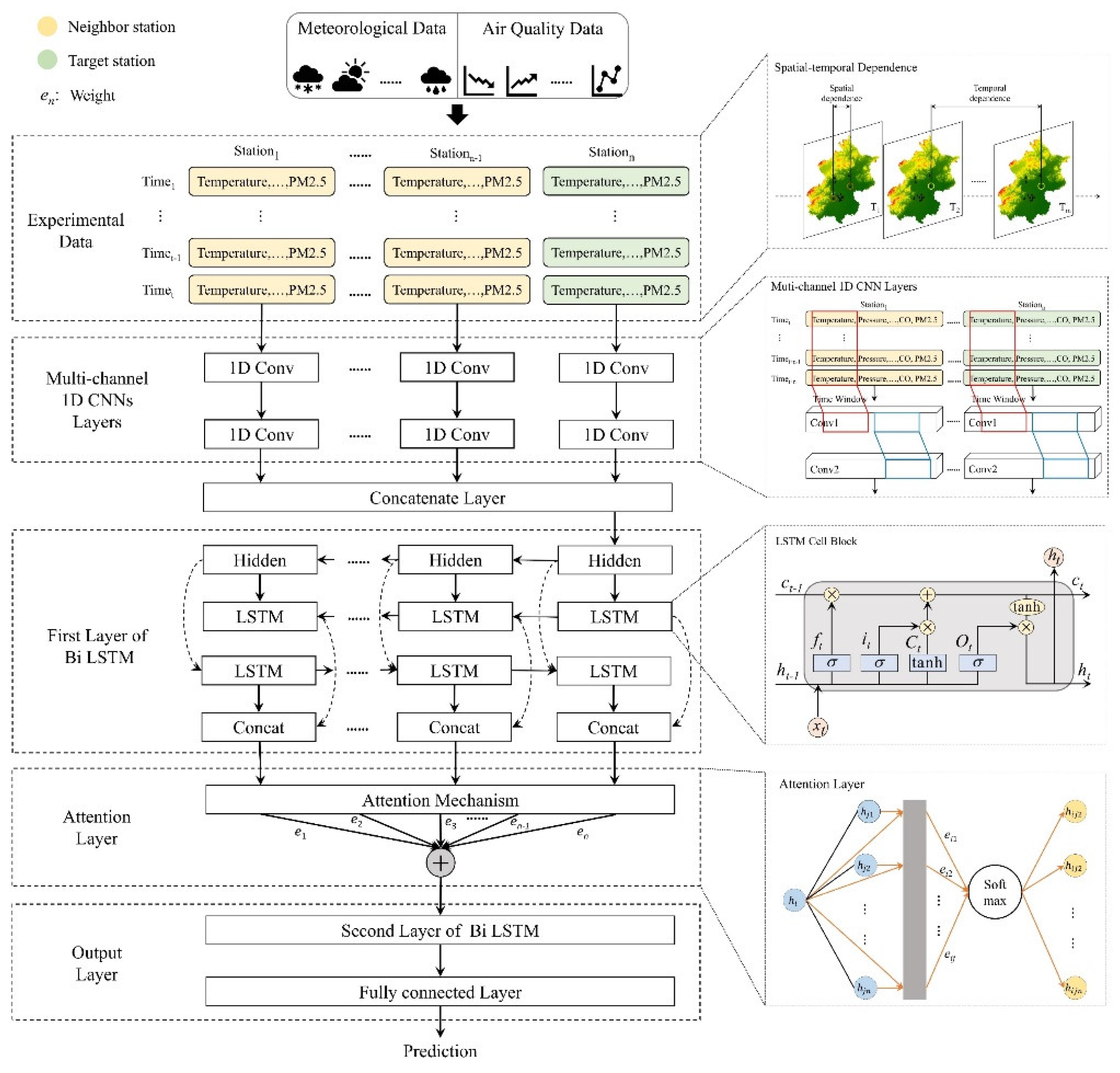
Figure 1. Structural components of the FPHFA model.
Applsci 12 11155 g001
Figure 2. Distribution of PM2.5 concentration monitoring stations.
Applsci 12 11155 g002
Figure 3. Time series plots of factors of influence.
Applsci 12 11155 g003
Figure 4. PM2.5 concentration in Beijing from 3 December 2016–28 February 2017. Seasonal variation of PM2.5 concentration (The picture on the left), Monthly variation of PM2.5 concentration (The picture on the right).
Applsci 12 11155 g004
Figure 5. Spatiotemporal distribution features of PM2.5 concentration.
Applsci 12 11155 g005
Figure 6. ACF and Partial Autocorrelation Function (PACF) plots for Actual Value (first row), ACF and PACF plots obtained with LSTM (second row), GRU (third row), CNN-LSTM (fourth row), DAQFF (fifth row), FPHFA (sixth row).
Applsci 12 11155 g006
Figure 7. Prediction step is 12 h, batch size is 128, and number of epochs is 40. Effect of window size on RMSE and IA of the models in the Beijing dataset. (a) RMSE, (b) IA.
Applsci 12 11155 g007
Figure 8. Window size is 56, prediction length is 12 h, and batch size is 128. Effect of number of epochs on RMSE and IA of models in the Beijing dataset. (a) RMSE, (b) IA.
Applsci 12 11155 g008
Figure 9. Predictions 12 h ahead in experiments on the Beijing dataset. The graphs compare one month’s worth of actual and predicted PM2.5 values (1 December 2016–31 December 2016) at station 1003A with different models. (a) LSTM; (b) GRU; (c) CNN-LSTM; (d) DAQFF; (e) FPHFA.
Applsci 12 11155 g009aApplsci 12 11155 g009b
Figure 10. Window size is 56, number of epochs is 150, and batch size is 128. RMSE, MAE, R2, and IA of models at different prediction sizes in the Beijing dataset. (a) RMSE. (b) MAE. (c) R2. (d) IA.
Applsci 12 11155 g010
Figure 11. Comparison between actual value and predicted PM2.5 value throughout the course of a month (16 December 2016–15 January 2017) for prediction steps of 24 h and 96 h, in experiments on the Beijing dataset, with different models (LSTM, GRU, CNN-LSTM, DAQFF, and FPHFA). (a1) LSTM model for prediction 24 h ahead; (a2) LSTM model for prediction 96 h ahead; (b1) GRU model for prediction 24 h ahead; (b2) GRU model for prediction 96 h ahead; (c1) CNN-LSTM model for prediction 24 h ahead; (c2) CNN-LSTM model for prediction 96 h ahead; (d1) DAQFF model for prediction 24 h ahead; (d2) DAQFF model for prediction 96 h ahead; (e1) FPHFA model for prediction 24 h ahead; (e2) FPHFA model for prediction 96 h ahead.
Applsci 12 11155 g011aApplsci 12 11155 g011b
Figure 12. Degree of fit between the observed and predicted PM2.5 value throughout the course of a month (16 December 2016–15 January 2017) with different models (LSTM, GRU, CNN-LSTM, DAQFF, and FPHFA) for prediction horizons of 24 h and 96 h, in experiments on the Beijing dataset. (a1) LSTM model for prediction 24 h ahead; (a2) LSTM model for prediction 96 h ahead; (b1) GRU model for prediction 24 h ahead; (b2) GRU model for prediction 96 h ahead; (c1) CNN-LSTM model for prediction 24 h ahead; (c2) CNN-LSTM model for prediction 96 h ahead; (d1) DAQFF model for prediction 24 h ahead; (d2) DAQFF model for prediction 96 h ahead; (e1) FPHFA model for prediction 24 h ahead; (e2) FPHFA model for prediction 96 h ahead.
Applsci 12 11155 g012aApplsci 12 11155 g012b
Table 1. Input variables for PM2.5 concentration forecasting models.
KindVar.UnitRange
Air Pollutant DataPM2.5μg/m3[2, 999]
PM10μg/m3[2, 999]
SO2μg/m3[0.2856, 500]
NO2μg/m3[1.0265, 290]
COμg/m3[100, 10,000]
O3μg/m3[0.2142, 1071]
Meteorological DataTemperature°C[−19.9, 41.6]
PressurehPa[982.4, 1042.8]
Dew Point°C[−43.4, 29.1]
Precipitationmm[0, 72.5]
Wind Direction [N, ESE]
Wind Speedm/s[0, 13.2]
Table 2. The model performance evaluation indicators of models in short-term PM2.5 concentration prediction.
ModelsRMSEMAER2IAMAPE
LSTM34.3923.030.79695.30%0.707
GRU32.6222.250.82495.93%0.683
CNN-LSTM31.6921.810.83296.15%0.672
DAQFF30.1221.020.84996.47%0.669
FPHFA28.1519.190.87797.04%0.561
Note: window size = 24, epochs = 100, and average of model performance evaluation indicators (RMSE, MAE, R2, and IA) over the next 1–12 h.
Table 3. The model performance evaluation indicators of FPHFA in long-term PM2.5 concentration prediction in comparison to other comparison models.
ModelsRMSEMAER2IAMAPE
LSTM33.9524.000.80495.53%0.831
GRU33.0123.330.81495.80%0.829
CNN-LSTM31.3222.140.83096.17%0.746
DAQFF29.1520.570.86496.83%0.691
FPHFA22.1215.270.93298.30%0.438
Note: window size = 48, epochs = 100, and average of model performance evaluation indicators (RMSE, MAE, R2, and IA) over the next 13–24 h.
Table 4. The model performance evaluation indicators of models in spring and summer.
ModelsSpringSummer
RMSEMAER2IARMSEMAER2IA
LSTM24.5817.530.85696.63%21.7816.190.66892.72%
GRU22.4515.760.87397.12%19.8714.790.71693.90%
CNN-LSTM21.0414.340.89697.55%17.8413.230.79195.32%
DAQFF20.2014.100.90597.76%19.0514.440.77194.73%
FPHFA15.8710.800.94998.71%13.189.780.91797.84%
Note: window size = 56, epochs = 100, and average of model performance evaluation indicators (RMSE, MAE, R2, and IA) over the next 24 h.
Table 5. The model performance evaluation indicators of models in autumn and winter.
ModelsAutumnWinter
RMSEMAER2IARMSEMAER2IA
LSTM23.7417.090.89697.50%32.4421.340.92898.29%
GRU23.3916.840.89097.48%33.4322.010.91598.08%
CNN-LSTM22.0615.320.91097.85%34.2421.560.91198.00%
DAQFF20.2214.530.92898.24%28.7017.740.95698.85%
FPHFA15.8611.050.95898.85%23.6914.930.96699.14%
Note: window size = 56, epochs = 100, and average of model performance evaluation indicators (RMSE, MAE, R2, and IA) over the next 24 h.
Publisher’s Note: MDPI stays neutral with regard to jurisdictional claims in published maps and institutional affiliations.