1. Introduction
Pavement distress initiation is closely related to the service life of the pavement and is usually accompanied by the deterioration of asphalt material and subgrade structural damage [
1,
2,
3,
4]. The presence of pavement distress not only accelerates pavement deterioration and reduces pavement life, but also affects driving safety and comfort to a large extent [
5,
6,
7,
8]. Pavement maintenance can effectively reduce pavement distress, and the common means of maintenance are mainly daily routine maintenance, major annual repair, and pre-maintenance. Since major annual repair and pre-maintenance require large investment in road refurbishment in a short period of time, the development of a corresponding maintenance plan is fully studied. The development of a maintenance plan requires observation and prediction for the initiation and deterioration of pavement distress. Pavement distress initiation and deterioration prediction based on long-term inspection records has proven to be an effective support for the development of major annual maintenance plans and pre-maintenance plans [
9]. In this paper, we distinguish between long term and short term and high frequency and low frequency, depending on the granularity of time. High frequency implies that data are collected at the daily or weekly level, and low frequency refers to data collected at the yearly level. Due to the lack of relevant datasets, the long term here is only restricted to refer to yearly data collected for many years. However, unlike major annual maintenance supported by a long-term pavement condition prediction model trained on large granularity data, daily maintenance needs the support of a short-time pavement distress occurrence prediction model. Higher frequency data collection can reveal more detailed correlations among variables, e.g., weather data in annual data are involved in modeling as static variables, while weather data at the daily or weekly level can be valued for their time-series properties in modeling. Therefore, in order to improve the efficiency of daily pavement maintenance, it is important to develop a short-time pavement condition generation prediction model.
Previous studies on predicting the occurrence of pavement distress have typically been based on long-term testing records, such as the Long Term Pavement Performance (LTPP) program [
10] and the AASHO road testing program [
11]. Sun [
12] concluded that the long-term deterioration trends of pavement condition index (PCI) and riding quality index (RQI) can be classified into four types, namely, concave, convex, inverse S, and pre-fast decay curves, based on the long-term observation data of five Chinese provinces, and the deterioration processes are represented by functional expressions. Loizos et al. [
13] studied the effects of construction, traffic, and climatic factors on pavement performance based on long-term pavement performance test data from 15 European countries and concluded that the log-normal function predicted the generation of pavement cracks most accurately. Dong et al. [
14] evaluated the generation time of road cracks based on data from the Long Term Pavement Performance (LTPP) project, and found that service life, traffic volume, and pavement structure are important in the crack occurrence process, while a survival model containing a Weibull hazard function is most relevant to describe various crack occurrences. The above studies explored the factors influencing crack occurrence based on long-term pavement condition data, which led to the construction of prediction models for pavement distress occurrence and deterioration, and these studies were useful for annual pavement condition prediction. However, daily routine maintenance requires a high-frequency prediction model for pavement distress initiation and deterioration, which means that prediction models must be trained using pavement distress data with small time intervals.
With the development of image processing technology in pavement surface distress detection, especially the accuracy of pavement surface distress detection and segmentation based on convolutional neural networks, detection has been significantly improved, and the automatic detection technology of pavement surface distress based on images has been gradually accepted and applied to pavement engineering [
15,
16]. Automatic detection of pavement surface distress usually loads a vehicle with a front-view [
17,
18] or rear-view [
19,
20] camera to capture images of the pavement surface. Convolutional neural network-based distress detection usually requires thousands of images to train the model [
21], and image data can be obtained from open source datasets [
22] or self-collected data [
23]. Subsequently, the pixel ranges with pavement distress are extracted from the original images by well-established image recognition frameworks, such as YOLO [
24], RCNN [
25], and transfer learning [
26]. YOLO and RCNN frameworks require larger single-scene datasets for training, and the accuracy for pavement distress detection in a single scene is higher, and the transfer learning framework requires more multi-scene datasets for training, so the robustness for pavement distress detection in multiple scenes is better. Finally, the detection of high-frequency continuous pavement distress occurrence and deterioration can be achieved due to the automation and low cost of pavement distress detection. Li et al. [
27] matched the pavement distress data collected on multiple consecutive days by constructing a spatio-temporal correlation algorithm to eliminate duplicate pavement diseases, thus achieving high-frequency continuous tracking of individual distress occurrence and deterioration. However, the abovementioned pavement distress detection techniques can only provide formatted information such as the classification attributes and appearance of geometric features of the pavement distress, and there is less research on how to analyze the characteristics of pavement distress’ short-period initiation and deterioration from these formatted data and construct a pavement distress short-period prediction model.
Similar to studies in environmental science [
28] and geophysics [
29] on the influence of physical systems by environmental factors, road pavements, despite their exposure to the natural environment, are not affected by the action of environmental factors in a simultaneous manner. Pu et al. [
30] used a long- and short-term memory (LSTM) neural network to develop a pavement friction prediction model based on daily pavement performance data collected over a long period of time, considering the time-series characteristics of pavement conditions, and found that the prediction accuracy was affected by the time lag and the prediction time interval. Brijs et al. [
31] used Dutch traffic data and weather data to construct count data models with temporal interdependence based on integer autoregressive models and found that daily changes in weather conditions had a significant effect on the number of crashes caused by changes in road conditions. However, fewer studies have focused on quantitatively studying the relationship between pavement distress generation and environmental factors. In the microstructure of pavement asphalt layers, Kettil et al. [
32] and Dong et al. [
33] found that the movement of moisture in the asphalt mixture due to vehicle loading under the influence of ambient temperature and humidity will reduce the strength and service life of the asphalt mixture. However, at the macroscopic level, most prediction models consider environmental factors as independent variables due to the lack of continuous decay detection data of pavement distress under natural conditions, and less consider the time series effect of environmental changes under short-period conditions, so it is meaningful for short-period pavement distress occurrence and deterioration prediction models to consider environmental factors.
This paper first established a pavement distress extraction framework to obtain the pavement distress initiation information. Combined with the geometric data and meteorological data, the pavement distress initiation dataset was set up to explore the daily change pattern and establish prediction models. Then, the time-lag cross-correlation analysis (TLCC) method was utilized to explore the time delay phenomenon in pavement distress initiation. The TLCC method is widely used to evaluate the influence factors in an environmental interaction system. Finally, the logistic regression results provide evidence that the time delay effect is useful to improve the model performance of the distress initiation prediction model.
The remainder of this paper is organized as follows:
Section 2 shows data collection and preparation.
Section 3 describes the methodologies of time-lag cross-correlation, variables correlation analysis, and logistic regression model.
Section 4 presents the results of correlation analysis and modeling.
Section 5 summarizes the findings, conclusions, and future work.
2. Data Preparation
Longwu Road, a Shanghai urban arterial road, was utilized as the study area. In China, arterial roads are the road grade second only to expressways in terms of traffic flow. The study area was set as ten sections in Longwu Road, which is a key road connecting downtown in Xuhui District, which means that its daily average traffic flow is at the forefront of the arterial roads. In this context, a section is defined as the road between two neighboring intersections. Longwu Road is oriented north to south and originates from West Longhua Road, and its destination is Huaji Road, with a total of 6.7 km in length.
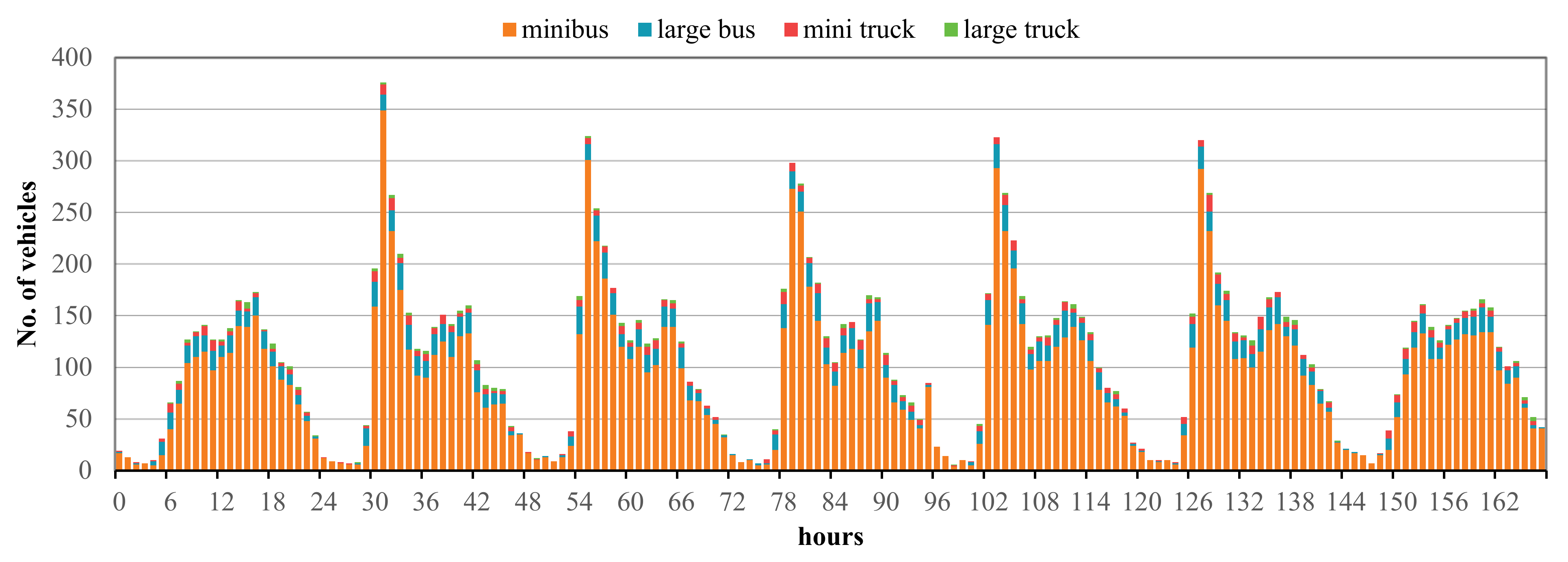
Longwu Road is a typical urban road. As shown in
Figure 1, the traffic flow statistics of a typical urban road intersection in Shanghai, its vehicle structure is usually comprised of minibuses and large buses. At the same time, there are a small number of small trucks and large trucks. The average daily traffic flow is relatively stable, except for the weekend traffic flow being less than that of weekdays. The daily traffic flow will not show large changes, so it can be assumed that the average daily traffic flow of Longwu Road will not produce too many sudden-change situations.
The pavement structure of Longwu Road is semi-rigid pavement. Specifically, there is a 4 cm SMA-13 (SBS modified) layer, 6 cm AC-20C layer, 7 cm AC-25C layer, 0.6 cm slurry seal layer, 48 cm cement-stabilized macadam layer, and 15 cm gravel sand layer. The pavement structure mentioned above is the most commonly utilized in Shanghai urban arterial road construction. Therefore, it can be inferred that the daily variation of pavement distress on Longwu Road is less affected by the variation of the average daily traffic volume and the variation of the pavement structure.
The study period was set from 21 January to 30 June 2021, totaling 161 days. During the study period, Shanghai underwent a transition from winter to summer, which means that the low-temperature and high-temperature conditions of the road are covered. Moreover, in the spring, the rainfall in Shanghai is intensive. So, the study period also covers the road surface conditions for the entire rainy season.
There were three data sources collected for this study: (1) pavement surface photographs data; (2) roadway geometric data; and (3) meteorological data. The pavement surface photographs data contain raw pavement surface images and corresponding raw GPS data. Then, combined with roadway geometric data and meteorological data, the pavement distress initiation dataset was established, shown in
Figure 2.
2.1. Detection of the Pavement Distress Initiation
The pavement surface photographs contain both the pavement distress information and coordinate information, which can be extracted from raw pavement surface images and raw GPS data. Raw pavement surface photographs were obtained by front-view cameras. Digital cameras were installed on vehicles’ roofs, which can obtain original pictures at a resolution of 1344 × 756 pixels. The input image pixel range is larger than the 512 × 512 pixel range of the commonly used pavement distress image datasets to satisfy the model training and detection requirements, and a larger image pixel range can improve the recognition accuracy but lead to longer detection time, so the current pixel range is more applicable [
34]. During image acquisition, vehicles drove through the whole study area daily. Raw GPS data including date, longitude, latitude, and azimuth were collected by the same vehicle.
Pavement distress has been extracted from raw pictures by an automatic method. An automatic pavement distress recognition and segmentation neural network, based on the YOLO_v3 framework, was established and trained to detect pavement distress information [
24,
34]. YOLO_v3 is a very widely used framework and is simple and robust enough to be used more easily in a variety of datasets, which means that the experimental procedure in this paper can be better reproduced. The YOLO_v3 framework uses pre-trained weights, while 45,788 images containing pavement distress collected in the same scenes are used for model training. The accuracy of cracks, potholes, and alligator cracks is 80.82%, 80.27%, and 91.38%, respectively, and the mAP of our model is 87.51%.
The detection results included pavement distress types (which contain transverse crack, longitudinal crack, alligator crack, and pothole) and bounding box (which part of the picture contains pavement distress), shown in
Figure 3.
Then, the latest distress pictures are matched and compared with the previous pictures as in the following steps.
Step 1: Determine the picture’s photographed direction. Calculate the absolute value of azimuth between the image and road direction. This paper defines road direction as the azimuth from origin to destination. Then, judge the photographed direction when the following criteria are satisfied:
where
and
represent azimuth of picture and road direction, respectively.
Step 2: Search the nearest picture obtained in the previous time step. For the pavement surface images in the same direction, calculate the Euclidean distance between the present pictures and images obtained last time. The previous images with the minimum Euclidean distance of the picture were set as the potential images containing initial distresses.
Step 3: Determine the initial time of pavement distress. A recurrent method was adopted for determining the initiation of distress. In the recurrent method, each picture labeled as ‘contain distress’ was inspected by civil engineers. To identify the initiation of pavement distress, the engineers compared the present pictures to the last period pictures in the same place. The classific rules for distress initiation include: (a) if a present picture contains distress and a last period picture is without distress, the distress initiation date was set as the acquisition date of the present picture; (b) if both the present picture and last period picture contain the same distress, the distress initiation date of the present picture was set as the distress initiation date of the last period picture; and (c) if the last period picture and its earlier period picture contain the same distress, step (b) should be applied until the distress initiation date is confirmed.
2.2. Independent Data Acquisition
Geometric data included road-section-adjacent road grade and the distance from image acquisition location to the nearest intersection center. Baidu Map API is open-source and offers integrated access to obtain geometric data in China. When the coordinates are input to the API, the distance between the coordinate point, the intersection, and the adjacent road grade will be returned. According to traffic volume, in China, the urban roads are divided into four levels: expressways, arterial roads, secondary truck roads, and branch roads. So, the distance to the intersection and road grade of adjacent roads at the same intersection implies the complexity of vehicles’ load patterns.
Weather data included maximum temperature, minimum temperature, daily average temperature, daily total precipitation, and relative humidity. The period of weather data is from 1 January to 30 June 2021, totaling 181 days.
Historical distress data contain the cumulative number of adjacent distresses. The length of the longitudinal crack is significant in the longitudinal direction of pavement and might impact the cumulative number of distresses in the adjacent area. According to the statistics of longitudinal cracks from the Long-Term Pavement Performance dataset [
35], the length of the adjacent area of the current coordinate was set as 50 m.
3. Methodology
To analyze the relationship between independent variables and disease generation, firstly, continuity analysis was performed on data with time-series properties, secondly, significance between categorical and numerical variables was explored, and finally, the relationship between independent and dependent variables was fitted to obtain the specific degree of influence. Compared with common temporal signal processing, such as dynamic time warping or instantaneous phase synchrony, time-lagged cross-correlation (TLCC) is not only possible to deal with temporal signals with many zero values, but also to obtain the correlation between peaks of different sizes, which is more applicable to the general pattern of pavement distress initiation [
36]. Traditional logistic regression models treat the coefficients of independent variables as fixed values. However, the Bayesian logistic regression model assumes coefficients follow a distribution [
37]. The generation of pavement distress has high uncertainty, and it is difficult to obtain a better fitted value by point estimate of parameters, while using the generation of pavement distress as a statistical distribution input can yield better predicted values.
3.1. Cross-Correlation Assessment
Cross-correlation is a common method for estimating the correlation between temporal information. That is, the correlation between two time-varying events may be consistent or inconsistent within the time interval. Two sequential time-series signals contain the same number of lead-follow relationships, and then the Pearson product-moment correlation is computed for the two signals. However, correlation analysis techniques do not provide information about synchronization between two signals, such as which signal leads and follows. TLCC has been used to identify relationships between two signals. TLCC is measured by gradually shifting the first signal and frequently calculating correlation with the second signal [
38,
39,
40]. The formula is as follows [
36]:
where
N is the sample size,
is the offset of signal,
and
are the values in two samples, and
and
are the mean of variables.
Windowed time-lag cross-correlation (WTLCC) is used to evaluate the cross-correlation during the whole time epoch. In various time series analysis methods, the assumption of the time-series variable is stationarity, which implies that statistical characteristics of time series are held across the entire time period. However, in some cases, the time-series statistical characteristics might be influenced by some factors. Therefore, window time-lag cross-correlation (WTLCC) is applied to assess whether the statistical features are stable by continuously adjusting the interval of the time windows [
36]. The measurement of windowed time-lagged cross-correlation between two signals is calculated in multiple time windows, and each window provides a score comparing the difference between the leader and follower signals.
3.2. Correlation Analysis
Time series analysis can provide time information between a pair of time series variables, but it lacks correlation analysis of all independent variables of the dependent variable. Understanding the degree of correlation between all independent variables helps to eliminate highly correlated independent variables in subsequent modeling and reduce the overfitting problem of the model.
Pearson correlation analysis is a common method to measure the similarity of a linear correlation between two numerical variables when a change in one variable is associated with a synchronization change in the other variable. If one dataset
X contains
n values and the other dataset
Y contains
n values, the Pearson correlation coefficient
r is given as [
41]:
where
n is the sample size;
and
are the values in two samples each indexed with
i;
and
are the variable values mean.
means a significant positive correlation,
means a significant negative correlation, and
means no correlation.
The Spearman correlation analysis is an appropriate method to assess the correlation between categorical variables (discrete ordinal variables) and numerical variables. The variable requirement is monotonic relationships (whether linear or not). The Spearman correlation coefficient is defined as the Pearson correlation coefficient between the rank variables, which can be computed as [
42]:
where
is the difference between two ranks of each variable,
and
represent the rank number in variable set
X and
Y, respectively, and
n is the number of sample sizes. Similar to the Pearson correlation coefficient, in the Spearman correlation coefficient,
means a significant positive correlation,
means a significant negative correlation, and
means no correlation.
3.3. Binary Logistic Regression Model
The aim of analyzing all influence factors is to find an ordinary way to describe the relationship between independent variables and dependent variables. In recent years, despite the rapid development of machine learning and deep learning, which have shown promising results in many fields, generalized linear models still have obvious advantages in terms of model interpretability in multi-factor modeling problems.
There are various regression models to establish the relation between the dependent variable and other independent variables. One of the methods is the linear regression model, but it is not efficient in modeling the binary dependent variable. The binary logistic regression model is a generalized linear model which can solve the modeling problem of the binary dependent variable. Binary logistic regression uses a logistic or logit transformation to link dependent variables to independent variables. The binary Bayesian logistic regression function is [
43]:
where
is the probability of
determined by the value of
x, and
is the probability of
,
n is the number of independent variables,
y is the binary dependent variable, and
P is the probability of the dependent variable,
represent the coefficients of each independent variable
to be estimated, and the coefficients
can explain the degree of the possible impact of independent variables on the dependent variable.
Each data category will be independently entered into the variables in the formula, and all categorical and numerical variables will be calculated with their respective statistical indicators, and then jointly calculated in the formula to obtain the corresponding coefficient values for the fitted minimum deviation. The coefficients of the independent variables of logistic regression can be calculated by maximum likelihood estimation. Similarly, the maximum likelihood estimation method can also calculate the probability of
y in the logit function. After the parameter estimation process, the significance of each parameter in the model can be calculated by the Wald test. The Wald test formula is [
44]:
where
is the standard error of coefficient estimation value of
b. A Python program was used to fit the formula and calculate the error.
4. Results and Discussion
4.1. Descriptive Analysis
The study time period was set from 21 January to 30 June in 2021. Hence, the first day of the study time period (21 January 2021) was set as the initial date of Longwu Road’s pavement condition. On the initial date, each observed distress was considered as the cumulative number of distresses before the study time period. During the rest of the study time period, each observed distress was processed via the image-processing approach and the distress-matching approach, and the pavement distress initiation variable could be calculated. There were 318 distresses observed on the initial date, and 809 distress initiations during the rest of the period. In this study, the non-initial distress value was chosen from the regular date, and the pavement surface image contains non-initial distress (including no distress and distress not occurring on that day). There were 810 non-initial distresses selected for further analysis. Therefore, a total of 1619 pavement distress initiation values were selected as the dependent variable in this study. The rest of the variables were utilized as independent variables, which could be divided into numerical and categorical variables.
Table 1 shows the summary statistics of all variables in the pavement distress initiation analysis dataset.
4.2. Temporal Cross-Correlation Analysis
The time lag is the time between two closely related events, such as cause and effect. The phenomenon of time delay in geography and environment was found as a common explanatory variable because interaction effects between various parts of the environment required an extended period. Moreover, some time delay effects were found in the previous research in pavement engineering and transportation. Road frost and anti-skid performance degradation caused by low temperature and high precipitation will not occur on the first day of the arrival of low-temperature weather but will occur after a short time delay [
30,
31]. To understand the effects of the environment including temperature, precipitation, and humidity, a time-lag analysis method with both time-lag cross-correlation (TLCC) and windowed time-lag cross-correlation (WTLCC) was utilized. The time-lag analysis results are presented in the following
Figure 4.
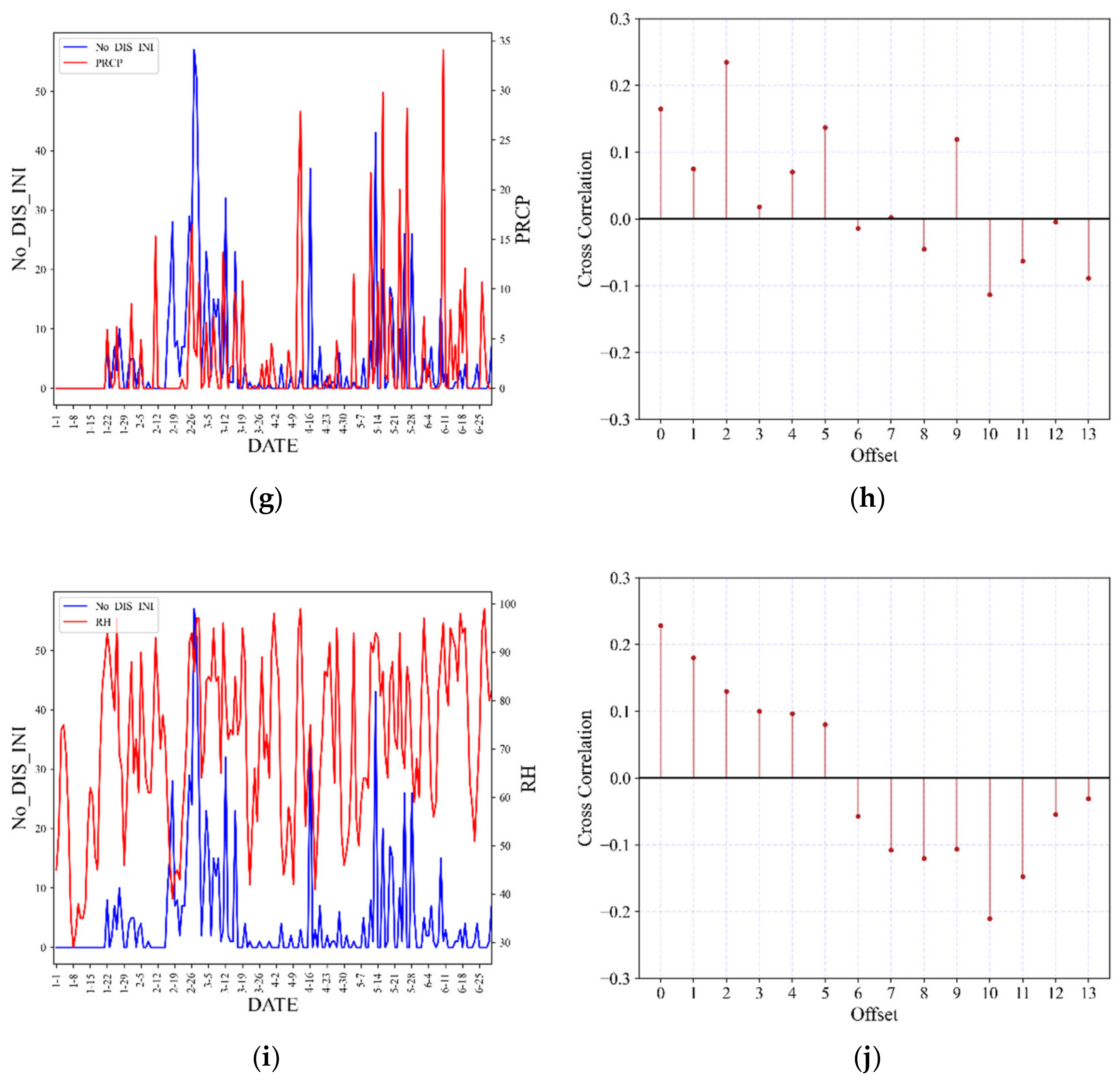
The daily cumulative number of distress initiations is presented in the left column of
Figure 4; the maximum value was observed on 26 February, and the maximum value is 57. The second-highest and third-highest daily cumulative number of distress initiations were 52 and 43, observed on 27 February and 13 May following 26 February, respectively. Moreover, two ridge types of the cumulative number of distress initiation variables in the broken line graph illustrate the concentrated outbreak of pavement distress occurrence. The first ridge started on 15 February and ended on 17 March. The time period of the second distress occurrence ridge was from 7 May to 1 June.
The broken lines from the meteorological variables in the left column of
Figure 4a,c,e are the daily change of maximum temperature, minimum temperature, and the daily average temperature, respectively. They all show high correlations and a significant increase during the study period, which offers an increasing temperature trend from winter to summer. In the left column of
Figure 4g,i, daily total precipitation and relative humidity were also observed with a slight increase during the study period. Significantly, the daily total precipitation variable has been observed in two ridges in March and May, respectively. It is illustrated that there were two concentrated rainfall periods in March and May during the study period.
The TLCC charts of each selected variable pair during the whole study period are shown in the right column. The horizontal axis of the TLCC chart is represented as the offset between two relevant signals, and the vertical axis is represented as the cross-correlation value, which measures the similarity of two relevant signals. In this study, the cumulative daily number of distress initiations was set as the S1 signal, and the meteorological variables were set as the S2 signal. The time-lag cross-correlation coefficient can be obtained by calculating the correlation between the S1 signal after shifting and the S2 signal. Therefore, the positive offset value means the S2 signal leads the S1 signal. The offset value represents the time interval in the above lead-follow relationship.
The TLCC chart of
Figure 4b shows the highest cross-correlation with zero time offset, and the correlation value is −0.10. It indicates that the maximum temperature might affect the distress initiation without time lag in daily time scales during the study time period. In
Figure 4d,f, the highest cross-correlation coefficients were observed in the positive offset equaling nine. The positive offset of 9 days had correlation values for the minimum temperature and daily average temperature of −0.14 and −0.12, respectively. It indicated that both weather variables above might affect the probability of distress occurrence after a 9-day interval. All three temperature-dependent variables have negative correlations between distress occurrence, with the time lag or without. The time lag of precipitation and relative humidity are two and zero, as shown in
Figure 4h,j. The highest correlation values of precipitation and relative humidity are 0.24 and 0.23. It can be inferred that the precipitation value might be highly relevant to the possibility of distress initiation two days later. Furthermore, the time lag between relative humidity and distress occurrence is a zero time interval. This indicates that distress initiation is more likely influenced by present relative humidity. At the same time, the correlation values of both precipitation and relative humidity are positive, which means a higher value would increase the probability of distress occurrence.
The WTLCC of relevant data was calculated to extract the change of temporal correlations between No_DIS_INI and each meteorological variable, as shown in
Figure 5. Each row value of the WTLCC charts represents the signals’ time series being divided equally into different parts of time epochs, and the cross-correlations were calculated in each window. The time-lag (offset) values of WTLCC were related to the results of TLCC values between the accumulation of distress initiations and meteorological variables shown in
Figure 5. The WTLCC of maximum temperature (
Figure 5a) showed that the correlation values with zero time offset are negative for most of the epochs from the beginning to the end time epochs. Moreover, the minimum temperature and the daily average of temperature in WTLCC charts (
Figure 5b,c) showed that the correlation values with the time offset of nine days were dominantly negative in all time epochs. Furthermore, the correlation value of relative humidity (
Figure 5e) showed positive values with no time lag from epoch zero to the end, which was similar to the result of TLCC (
Figure 4j). Finally, the correlation coefficient of the daily average of precipitation with a two-day time lag showed slightly negative values for most of the time epochs, despite two highly correlated values being observed. One reason for the result is that the precipitation signal contains too many zero values, and too many zero values might be dominant in the WTLCC value if time windows are in small intervals.
4.3. Correlation Analysis
The time-lag phenomenon has been extracted from the relationship between pavement distress initiation and meteorological data in the above analysis, but the effect of the time delay in predicting distress initiation should be further discussed. Therefore, the binary Bayesian logistic regression model should be established to assess the contribution of the time delay effect by considering time lag in weather variables’ value.
Based on the preliminary temporal correlation analysis results, the weather variables considered the time delay effect by setting a time lag in variables’ value calculation. The time lags of maximum temperature (MAX_TEMP_LAG), minimum temperature (MIN_TEMP_LAG), the daily average temperature (AVG_TEMP_LAG), daily total precipitation (RH_LAG), and relative humidity (PRCP_LAG) were set as zero, 9 days, 9 days, 2 days, and zero, respectively. Specifically, the value of the weather variables with time-lag t means the meteorological variable’s value t days ago. For example, the precipitation variable on 16 May was 29.8 mm, and the precipitation variable with a 2-day time lag was 10.7 mm on 14 May. Therefore, the rest of the weather variables with time lag can be obtained with the same approach.
Figure 6 presents the correlation coefficients of seven numerical variables with the pavement distress initiation. The red and blue boxes in the correlation coefficients matrix indicate that the counterpart variables have positive and negative correlations, respectively. The color depth indicates the level of positive and negative correlations. Three light blue boxes in the cumulative number of distress initiations column illustrate that maximum temperature, minimum temperature, and the daily average temperature during the study period have negative correlations with pavement distress initiation, which means the probability of distress occurrence would decrease if the temperature-dependent numerical variables go up. Significantly, the three deep red boxes illustrate that maximum temperature, minimum temperature, and the daily average temperature have remarkable positive correlations, which is easy to understand provided that daily average temperature was calculated with maximum and minimum temperature. So, to reduce the effect of highly relevant variables in regression modeling, the daily average temperature was considered in the modeling, and the maximum and minimum temperatures were excluded. Moreover, two light red boxes in the cumulative number of distresses column under the temperature boxes illustrate that daily total precipitation and relative humidity negatively correlate with distress initiation. It can be described as higher precipitation values, and relative humidity leads to a higher possibility of distress initiation, which means more moisture content in the atmosphere might cause pavement surface conditions to deteriorate. Furthermore, the distance between the current coordinate and the nearest intersection negatively correlates with distress initiation via a light blue box. Significantly, the box between the distance from the current coordinate to the nearest intersection center (DIS_NEAR_INT) column and the cumulative number of distresses within 50 m of the current coordinate (No_ADJ_DIS) column is light blue, illustrating that distance increases between the current coordinate and the nearest intersection would reduce the cumulative number of pavement distresses. Moreover, the light blue box between the ‘DIS_NEAR_INT’ column and PD_INI column indicates that distance increases between the current coordinate and the nearest intersection would lead to a lower probability of distress initiation. In addition, the light red box between the ‘NO_ADJ_DIS’ column and ‘PD_INI’ column shows the current coordinate has more distresses and would be more likely to generate new distresses in the future.
The correlation coefficients of two categorical variables with the pavement distress initiation are listed in
Table 2. The correlation matrix shows that correlation coefficients of pavement distress initiation with the road grade of neighboring upstream and downstream roadway sites are 0.046 and −0.039, respectively. This implies that pavement distress initiation might have a different probability even under the same meteorological condition and similar pavement surface condition due to the difference between the neighboring road grade of road sections in the upstream and downstream direction. Considering the definition of road grade related to the traffic volume, it can be inferred that slight variation in traffic volume caused by neighboring roads has weak correlations with pavement distress initiation, based on the low correlation coefficients with distress initiation. On the one hand, it might cover the reality of traffic volume by estimating traffic volume with classes of road grades because of the strong correlation between traffic volume and pavement condition deterioration [
4]. On the other hand, it might have a small traffic volume change caused by neighboring roads because 7 in 10 neighboring roads are secondary truck roads and branch roads that operate in a low-service traffic volume. Hence, it might be important to record the numerical value of the real traffic volume for pavement distress initiation prediction in daily routine road maintenance.
4.4. Logistic Regression Analysis Results
We assessed the time delay effect in predicting pavement distress initiation by comparing Bayesian logistic regression models with or without time-lag variables. The first Bayesian logistic regression model considered variables including geometric data (UP_RD_GRADE and DOWN_RD_GRADE, DIS_NEAR_INT), historical distress data (NO_ADJ_DIS), and meteorological data, which considers the time delay effect. On the contrary, the second Bayesian logistic regression model considered variables including geometric data, historical distress data, and meteorological data without time lag.
The pavement initiation dataset was randomly split into train and test datasets with a ratio of 70:30. Then, the Akaike information criterion (AIC), Bayesian information criterion (BIC), and the area under the receiver operating characteristic (AUC) curve were selected to assess the model performance. A lower AIC indicates a better model performance with simple parameters. The AUC range is from 0.5 to 1.0. A higher AUC represents a better potential precision ability. When the AUC range is from 0.7 to 0.8, it indicates the model performance is acceptable, and if the range is from 0.8 to 0.9, this means the model is a good fit of the dataset, and if AUC is higher than 0.9, this indicates perfect prediction.
The results of the logistic regression model are shown in
Table 3. The values of AIC and BIC for the model with weather parameters with time lags (model 1) are 1335.703 and 1375.964, both of which are smaller than 1371.775 and 1412.036 for the model without considering weather parameters with time lags (model 2). The values of AIC and BIC are determined by considering both the complexity of the model and the likelihood function, and taking the model likelihood function is considered as a penalty term, which means that the model complexity and prediction accuracy are most balanced when the AIC and BIC are smallest [
45]. Therefore, the introduction of the time-lag relationship makes the model performance of the prediction model better. Similarly, from the AUC values of 0.759 and 0.761 for the training and test sets of model 1, which are both better than 0.748 and 0.749 for model 2, it can be found that introducing the time-lag relationship can improve the prediction accuracy of the prediction model.
In addition, the variables of weather factors (average daily temperature, total daily precipitation, and relative humidity) showed significance in the logistic regression model with or without time-lag characteristics, and the conclusions of the correlation analysis can be analyzed together to know that weather factors still play a non-negligible role in the prediction of short-term distress initiation, despite their relatively small influence. Similarly, the distance to the nearest intersection and the pavement distress accumulation in the adjacent area also showed significance in the logistic regression model, which corroborates with the high correlation between the two variables and distress initiation in the previous correlation study. On the contrary, in the logistic regression model, the significance of the grades of the upstream and downstream adjacent road sections was not significant, possibly because this variable is an indirect response to the traffic volume of the road section, which does not correspond to the actual traffic volume and, therefore, does not show significance in this study.
The logistic regression model reflects the degree of influence of the variable parameters on the predicted values by means of probability ratios. For example, the cumulative number of distresses within 50 m of the current coordinate (No_ADJ_DIS) parameter shows a highly significant coefficient equal to 0.1591, which indicates that the probability ratio of pavement distresses’ occurrence will increase by 1.172 (equals to e to the 0.1591) times when the number of historical distresses increases by one. All significant variables in both models showed the same trend and differed only in their values, showing the correctness of the prediction models. Among the weather factors, the coefficients of daily average temperature and relative humidity are similar in both models, while the coefficient of daily precipitation in model 1 is 0.046 greater than that of model 2, which indicates that the consideration of time lag on daily precipitation will have a greater impact on the prediction accuracy of distress generation.
5. Conclusions
Previous research has focused on establishing relevant prediction models and exploring the impact of multiple factors on the initiation and deterioration of pavement distresses through long-term data. This paper used road image data with a short collection period to predict the initiation of pavement distresses and explore the relationship between the changes in various weather factors and the initiation of distresses. The conclusions obtained are as follows:
(1) The time-lag cross-correlation analysis was processed between initiation of pavement distresses and maximum temperature, minimum temperature, daily average temperature, daily total precipitation, and relative humidity. It can be found that the correlation of the number of distress initiations between the maximum temperature of the day and relative humidity at the same time is −0.10 and 0.23, respectively. Moreover, the correlation of distress initiation between minimum temperature nine days ago, daily average temperature nine days ago, and daily total precipitation two days ago is 0.14, −0.12, and 0.24, respectively. This indicates that the impact of temperature and precipitation on road distress initiation has a time-lag effect;
(2) Through the analysis of the correlation between the number of pavement distress initiations and the related factors of road alignment, it can be known that the coefficient of initiation of road distress and the distance from the pavement to the intersection center is −0.17, which means there is a negative correlation. Moreover, the coefficient is 0.26, which means there is a positive correlation with the number of historically accumulated distresses on the pavement. However, since the coefficients are both below 0.01, the initiation of pavement distress has a weak correlation with the road grade of the neighboring road;
(3) Binary logistic regression models with or without time-lag variables were utilized to establish a distress initiation prediction model and explore the degree of influence of each variable on distress initiation. The weather factor variables of one model consider the influence of the time-lag effect, while the weather factor variable of the other model does not consider the impact of the time-lag effect. The AIC and BIC of the model containing time-lag variables are 1335.703 and 1375.964, both lower than the other, revealing that the first model is more precise than the second model. The modeling results show that the AUC of the training and testing sets in the model considering time lag is 0.759 and 0.761, respectively, indicating that the weather factor variables considering the time-lag effect could help improve the prediction of pavement distress initiation accuracy.
Based on the research of this paper, the following research can be carried out in the future. Firstly, in the temporal aspect, the time range of image acquisition for pavement distress can be extended to improve the robustness of the results. By extending the acquisition time range of the dataset to more than one year, the differences in predicted data under the same monthly and quarterly data from different years can be explored by experiencing weather changes in a complete year, and the estimation bias of model parameters can be reduced. Secondly, in the spatial aspect, the regional span of pavement distress image acquisition can be expanded to improve the adaptability of the conclusions. Studying the pavement distress initiation under different traffic volumes under the same type of area can help explore the anomalies of distress generation due to traffic characteristics (e.g., road sections with more heavy vehicles) or explore the differences of various road classes on distress generation. Due to the generality of the method in this paper, the trending conclusions on weather and geometric factors on distress generation can be applied to more areas. However, the weather values vary from region to region and the coupling relationships between weather factors are complex, so a larger number of collections from different regions may lead to a more numerically general model.


