Abstract
RFID systems are often used in industry to reduce costs, increase process efficiency and minimize human intervention. The challenge is to design an RFID system before it is implemented in a specific environment in the shortest possible time and at minimum cost while maintaining the accuracy of the results. In this paper, a new approach to predicting indoor UHF RFID signal coverage is presented. It is based on a graphical ray tracing method. Simulations are performed based on spatial analysis of the illumination of a 3D indoor environment created from a 2D floor plan. The results show a heat map representing the predicted RSSI radio signal levels using a color range. The approach is validated by comparison with the results of the empirical Multi-Wall model. The time complexity of the approach is presented. The proposed approach is able to generate a heat map with the accuracy of the empirical Multi-Wall model. The interior room equipment required to refine the results ought to be investigated in the future.
1. Introduction
Applications using passive RFID (Radio Frequency Identification) technology, especially in the UHF (Ultra-High-Frequency) spectrum, are encountered in many sectors of operation nowadays. It is especially the identification and localization of objects and people in indoor space [1,2,3,4], logistics and inventory [5,6,7] or the monitoring of pipeline defects [8] in order to improve performance and efficient productivity and to increase service quality. An RFID system typically consists of a reading device, i.e., an RFID reader with a set of antennas and RFID tags that store information about a product or service. A larger number of readers and tags together form a complex system for identifying, tracking and monitoring objects bearing RFID tags. In this paper, the focus is on passive RFID communication in the UHF band 860–960 MHz, where the energy to activate the RFID tag is obtained from the reader device. Thus, the reading area depends mainly on the power radiated by the reader, the sensitivity of the tags, the orientation of the antennas and the shape of the area of operation of the system [9].
For passive UHF RFID systems, a difficult problem is to design the optimal placement of these RFID systems so that the desired area is completely covered by the signal. The tags have to be activated by the reader, and at the same time, there is no unwanted interference between the reader and the tags, which could lead to service degradation and reduced quality or error conditions. Another problem is the operation of the RFID system in the UHF band, where influences related to the environmental properties are typical and can have a strong impact on the performance of the system [10]. Furthermore, when designing the system, the parameters of the reader, antenna and tags must be taken into account, as well as the practical implementation (cable lengths, availability of electricity, etc.) [11]. Last but not least, other telecommunications technologies that can be operated in a given location in the same frequency spectrum should be considered to avoid undesired interference when designing an RFID system [11].
For the design of the RFID system, in terms of the accuracy of the results, physical measurement or on-site experimentation, which allows for obtaining accurate values of the measured parameters, appears to be suitable. From the physical measurements, we can mention, for instance, the determination of the required power (strength of the electromagnetic field) of the antennas of RFID readers by placing the tag in the space and measuring their detectability by the reader. The values of the RSSI (Received Signal Strength Indicator) parameter of the tag response at a constant power of the RFID reader can be recorded in order to determine the reading range of RFID UHF readers or antennas [11]. However, this procedure seems to be inappropriate in terms of time and money consumption. As a suitable solution, the use of simulation tools allow the placement of RFID components in 2D or 3D space. The simulation allows the implementation of various scenarios, such as the prediction of tag coverage (detectability), the effect of signal attenuation on obstacles, reflections from surfaces and others [12]. Such simulations can then help, for instance, in tuning the performance of RFID readers and thus in estimating the signal range for tag activation. The results of these simulations can have comparable predictive value to physical measurements and can thus provide a basis for physical implementation.
Over the last decades, several methods have been proposed to simulate the propagation of electromagnetic waves ranging from extremely low-frequency (ELF) [13] to terahertz waves [14]. The authors of article [15] divide these methods into three categories: empirical methods, deterministic methods (full-wave simulation) and ray tracing. Empirical methods, such as One-Slope [16], Dual-Slope [16], COST-231 [16] or Okumura-Hata [17], are based on a large number of measurements but may be inaccurate in the case of atypical spaces. For the application of RFID deployment in an indoor area, these methods lack spatial information and energy changes due to multipath propagation, which is very important for defining the tag readability area [15]. Among the deterministic methods, Method of Moments (MoM) [18], Finite-Difference Time-Domain (FDTD) numerical method [19] and Finite Integration Technique (FIT) numerical method [20] are mentioned. These methods are accurate but are computationally complex and time-consuming [15]. As a compromise, the now widely used deterministic method ray tracing [15,21,22,23,24,25,26,27,28,29,30], more precisely, ray tracing (physics) (RT), is based on geometrical optics (GO). It is usable as an approximated method to estimate the intensity of an electromagnetic field [21]. In this method, electromagnetic waves are treated as rays. The principle is based on emitting a certain number of rays from a source and tracking them. These then interact with obstacles in the form of refraction, diffraction and reflection depending on the material of the object, and so attenuation occurs at the obstacles [21]. In an indoor environment, the material represents a large part of the influence on attenuation. In RT simulations, the material properties of all objects within the simulation are often taken into account based on the knowledge of the dielectric constant and permittivity in the range of operating frequencies [31]. For instance, the authors in [32] discuss the calibration of ray tracing models based on measurements of permittivity and conductivity in the indoor environment. The limitations of this method are mainly the number of rays emitted and the size of the surfaces on which the rays hit and on which the resulting intensity is subsequently calculated and correlated. In the first case, the calculation time increases with an increasing number of rays, and in the second case, inaccuracy in the calculation may occur due to the different number of incident rays [33].
RT is a frequency-independent and widely used method for 2D and 3D radio coverage prediction. Therefore, it is often implemented as a feature in software tools. Some of the frequently used tools include Altair WinProp [34], Wireless InSite [35] and Altair Feko [36]. The authors of [37] use a combination of Altair Feko and Altair WinProp to predict the coverage of an indoor RFID infrastructure. The authors of [21] study the coverage of UHF-RFID tags at 433 MHz in an indoor environment using Altair WinProp. The authors of [22] use Wireless InSite as a 3-D ray-tracer to evaluate the proposed tag placement algorithm for THz RFID. The papers are categorized in Table 1.

Table 1.
Categories of papers.
An analog of the physical ray tracing method is encountered in the domain of computer graphics as a technique for generating images in computer graphics. It belongs to the group of so-called global illumination algorithms, further referred to as ray tracing (graphics) (RTg). This method can be considered as a possible approach to predict the coverage of the radio signal in the graphics domain. The equation that describes the propagation of light in a 3D scene (i.e., the rendering equation) was published by James T. Kajiya in 1986 in [38].
The aim of this paper is the verification of the use of the RTg algorithm for the simulation of radio signal propagation in a 3D indoor environment for UHF RFID technology. The investigation of this approach is the main contribution of the paper because the RTg algorithm solves the global illumination problem in the domain of computer graphics by default. In the simulation, the effect of reflections and refractions, where some parameters, such as the shape of the 3D environment and the influence of materials, are considered. The simulation results of this approach are compared with the results of simulations of the empirical Multi-Wall model used in the simulation tool I-Prop [11]. For the presented approach, we focus on verifying the functionality, repeatability, accuracy of the results and time consumption.
Considering the simulation results, it can be concluded that this approach is applicable to simulate the UHF signal coverage from an RFID reader in an indoor environment. The authors of [11] compare the results of the Multi-Wall model with the real measurement results. Based on the p-value in the ANOVA table being less than 0.01, the authors conclude a statistically significant relationship between the results. Comparing the two original and two simulated heat maps, the maximum difference is 6.7% in the range of RSSI values −20 to −30 dBm for antenna 1. In terms of the highest and lowest differences for RSSI ranges, it is 6.5% in the range −1 to −20 dBm and 0.9% in the range −80 to −100 dBm for antenna 1. The total time to create the simulated environment is less than 10 min and the simulation time to create the heat map is less than 1 min.
The rest of this paper is structured as follows: Section 2 describes the approach to the simulation with all the required settings. The results from the heat map comparison and the discussion of functionality, repeatability, accuracy of the results and time consumption of this approach are presented in Section 3. The conclusion of this paper is presented in Section 4.
2. Methods
For the design principle of this method, a combination of two tools is chosen. The SketchUp Pro 2021 software tool allows the creation of a 3D model of the indoor environment. The advanced multi-core ray tracing engine called V-Ray is a plugin of SketchUp Pro, which uses the ray tracing (graphical) method. This combination allows the entire simulation to be created in one framework. That is, creating a 3D scene based on the floor plan, setting up sub-components for the heat map simulation, such as materials or lights, and rendering the final heat map output on the layer of floor plans with the corresponding RSSI values. The complete process of creating a 3D scene up to heat map generation is shown in Figure 1 and is explained in detail in Section 2.1, Section 2.2, Section 2.3, Section 2.4, Section 2.5, Section 2.6, Section 2.7 and Section 2.8.
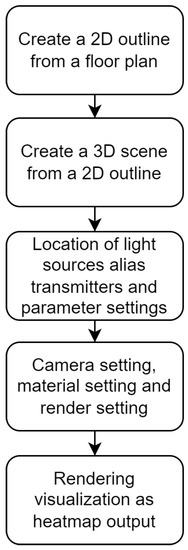
Figure 1.
Procedure for creating heat maps.
2.1. RTg Method
Ray tracing (graphics) as a method for image generation by tracing the paths of light (rays) from the camera through pixels in the image plane is used in this approach; see Figure 2. The effects of rays encountering virtual objects are simulated.
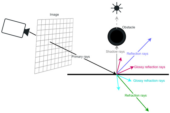
Figure 2.
The basic mechanism of RTg.
The procedure of RTg is described in the following steps:
- Primary rays—traced from the camera into the scene determine what will be seen in the final image.
- Shadow rays—traced from each rendered point to each light in the scene determine whether the point will be illuminated or shadowed.
- Reflection rays—traced in the direction of the reflection vector, which depends on the type of reflection, i.e., fresnel or normal and the index of refraction of the material.
- Refraction rays—the direction of the rays depends only on the index of refraction of the material.
- glossy rays—many rays are traced in a cone, and the distribution of the cone depends on the amount of gloss of the material.
2.2. Selecting the Environment for Simulation
For the purpose of comparing the simulation results with existing simulated values, the authors’ indoor corridor environment in [11] is chosen. The following parameters needed to create the same environment are known:
- Floor plan of the area,
- Location of RFID readers (antennas),
- Heat map on 2D floor plan with corresponding RSSI values.
With these parameters, the outputs of the approach presented in this paper can be compared with the empirical Multi-Wall method used by the authors of [11]. The original floor plan is shown in Figure 3. The heat map over the floor plan with RSSI values is shown in Figure 4 for antenna 1 and Figure 5 for antenna 2.
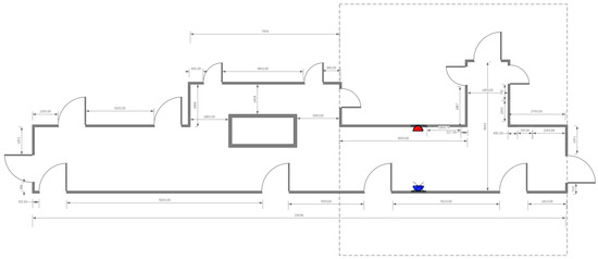
Figure 3.
Original floor plan, taken from [11].
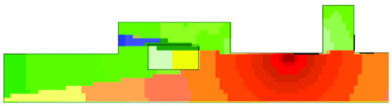
Figure 4.
RFID signal propagation for antenna 1 in the corridor, taken from [11].
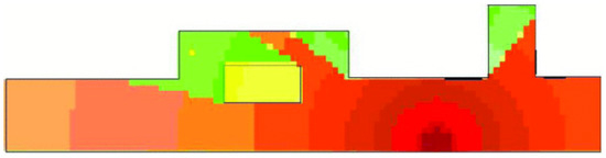
Figure 5.
RFID signal propagation for antenna 2 in the corridor, taken from [11].
2.3. Selecting of Software Tools for Simulation
SketchUp Pro 2021 software tool is chosen for the creation of 3D indoor environments as a 3D architectural design tool with accurate metric mapping of physical space to virtual space. The V-Ray software add-on is used for the resulting heat map scene visualization, which is implementable as a plugin in the SketchUp tool. The V-Ray software is a multi-core ray tracing engine that is focused on fast and accurate visual results using the RTg method. The main feature of V-Ray is the VRayLightingAnalysis (VLA) renderer. It allows the analysis of the illumination intensity on 2D surfaces and in 3D space and creates a visual heat map in the environment. This map is generated with a smooth color transition representing a range of light intensity, from blue (low intensity) to red (high intensity). These color ranges can be compared to the range of RSSI color spectrum values; see Figure 6, used by the authors of [11].
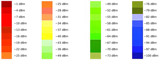
Figure 6.
Color spectrum representing the RSSI values in the heat map used in the simulation, taken from [11].
2.4. Creating 3D Simulation Model
A floor plan is selected for modeling; see Figure 3. The 3D model is created in SketchUp in accordance with the floor plan; see Figure 7. The only unknown is the ceiling height, which has been set to 3 m, which we consider a sufficient compromise given the fact that only one floor is considered.
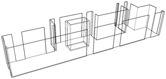
Figure 7.
Three-dimensional model of the corridor from the floor plan in SketchUp.
2.5. Sources of Signals
For the simulation, two light sources from the V-Ray Sphere Light are placed in the 3D scene in accordance with the original RFID antenna placement; the red dot is for antenna 1, and the blue dot is for antenna 2; see Figure 8. These light sources replace the original RFID antennas; see Figure 4 and Figure 5. These light sources can be compared to the properties of an isotropic emitter. See Table 2 for the original antenna settings and Table 3 for the settings for the light sources.
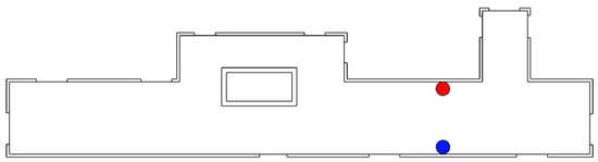
Figure 8.
Position of light sources in the scene. Red dot for antenna 1, blue dot for antenna 2.
Table 2.
Parameters of the RFID antennas.
Table 3.
Parameters set for V-Ray Sphere Lights.
The default SunLight function is disabled in the 3D scene and the Shadows, Affect (Diffuse, Specular, Reflections) functions are left unchanged in the “On” state.
2.6. Material Setting
Commonly used ray tracing simulation tools work with material properties for a specific frequency range, i.e., permittivity and conductivity coefficients. As this approach is based on the RTg method, light rays are used instead of interpreting electromagnetic waves and materials need to be modified accordingly to simulate the effect of electromagnetic properties on materials. The use of glass material (i.e., VRAY Glass material) seems to be appropriate. This material is applied to all objects in the scene with the following parameters:
- Diffuse color—rgb(255,255,255)
- Reflection color—rgb(255,255,255)
- Refraction color—rgb(204,204,204)
- Index of Refraction (IOR)—1.52
- Reflection Max Depth—5
- Refraction Max Depth—5
The diffuse color parameter set like this indicates that the material has white color as the default. The IOR parameter represents the glass material and indicates that light rays interact with the surface for ideal refraction and reflection. The reflection color parameter specifies the amount of reflection. The refractive color parameter allows the generation of the attenuation of optical rays due to the change in light transmittance of a given material. The authors of [11] give an attenuation due to walls of 14 dB, and this attenuation approximately corresponds to the above settings found by simulation. The maximum depth of reflection and refraction indicates how many times the ray can be reflected or refracted. This value is set by default for the VRAY Glass material, and increasing these values results in higher computational complexity. The maximum value of reflections and refractions is limited to 10 in this SW.
In terms of material limits, these limits can be specified as:
- Refraction color—rgb(0,0,0) (non-transparent)
- Refraction color—rgb(255,255,255) (fully transparent)
- Reflection color—rgb(0,0,0) (non-reflective)
- Reflection color—rgb(255,255,255) (fully reflective)
2.7. Camera and Render Setting
For the camera setting, the top view is chosen with an orthogonal view in accordance with the original heat map, Figure 4 and Figure 5. It allows a comparison between the original and the generated heat map under the same conditions.
The rendering settings are configured to generate a heat map, and the processor is selected as the computational unit. It is common today to use a graphics processor to render computer graphics, but the VLA renderer does not currently support this option. The details of each setting can be seen in Figure 9.
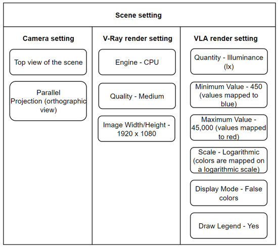
Figure 9.
Scene settings for correct heat map rendering.
2.8. Comparing Heat Maps Using Pixel Presence in the Heat Map
The results of the RTg method, i.e., the simulated heat map shown in Figure 10a and Figure 11a, are compared with the empirical Multi-Wall method, i.e., the original heat map shown in Figure 10a and Figure 11b. The comparison is performed by the Python script [39]. The input of this script is the original and the generated heat map, but it is mandatory to unify the orientation and resolution of both heat maps. RTg and the VLA renderer used allows for the generation of heat maps with a smooth color spectrum of RSSI values, see Figure 10a and Figure 11a, which is desirable in the case of more accurate coverage prediction in units of RSSI values. In the case of the comparative heat map; see Figure 10b and Figure 11b, the resolution of RSSI values is not as fine. This is taken into account in the comparison of the simulated heat maps.
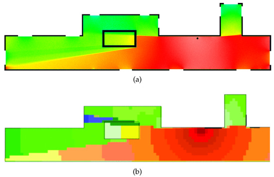
Figure 10.
RTg heat map of antenna 1 (a) and Multi-Wall heat map (b) (taken from [11]).
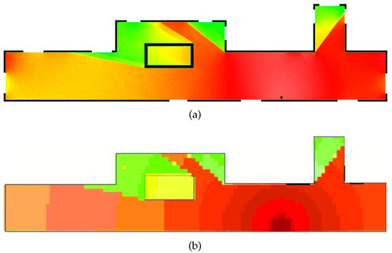
Figure 11.
RTg heat map of antenna 2 (a) and Multi-Wall heat map (b) (taken from [11]).
A smooth color spectrum of RSSI values shown in Figure 12 is loaded into the script based on the RSSI values from the I-Prop tool, Figure 6. A set of color ranges corresponding to the ranges of RSSI values is then created. The script then detects the color of each pixel and assigns it to a color range of RSSI values. The result is the percentage representation of each RSSI value or range of RSSI values from both heat maps, i.e., simulated and original. White, black and grayscale colors are not considered RSSI values and are excluded from the detection. From the original RSSI gradient values shown in Figure 6, it can be seen that the color ranges for −1 to −20 dBm are considered to be red. The shades of blue are considered equal in the −80 to −100 dBm range. The shades of green are found in the −40 to −60 dBm range, and thus, this fine differentiation disappears for this reason, the classification of the ranges is proceeded with:
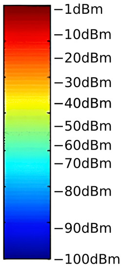
Figure 12.
Smooth color gradient of RSSI values created from the template according to Figure 6.
- −1 to −10 dBm and −10 to −20 dBm is unified as −1 to −20 dBm
- −40 to −50 dBm and −50 to −60 dBm is unified as −40 to −60 dBm
- −80 to −90 dBm and −90 to −100 dBm is unified as −80 to −100 dBm
The evaluation of the matching tool in Python follows values of 10 dBm, i.e., −1 to −10 dBm etc.
3. Results and Discussion
3.1. Functionality and Repeatability
The evaluation criterion in terms of functionality is the ability of this approach to generate a heat map representing the electromagnetic (EM) signal intensity, which is based on the knowledge of the 3D form of the simulation environment, Figure 10a and Figure 11a. This approach is validated against the heat map generated by the I-Prop tool, which uses the Multi-Wall method, Figure 10b and Figure 11b. The functionality fulfills the evaluation criteria.
The repeatability is verified by generating two different heat maps, i.e., for antennas 1 and 2, while keeping the same parameter settings. The simulated heat map results are similar (equivalent) to the simulations generated by the Multi-Wall method for both scenarios.
3.2. Accuracy of the Results
The results of heat map comparison using RSSI color ranges are shown in Table 4 for antenna 1 and Table 5 for antenna 2. For antenna 1, it can be seen that there is about a 6.5% difference in the ranges −1 to −20 dBm and −20 to −30 dBm. Looking at the original and simulated heat maps, Figure 10a and Figure 11a, the simulated heat map lacks the orange color at the circular distance from the antenna. It is replaced by the red color of the higher-intensity RSSI values. This is due to the fact that for the RTg method, the level of the transmitted signal does not decrease with distance from the source at the chosen setting with such a steepness as in the case of the Multi-Wall method. The remaining differences are less than 1.6%.
Table 4.
Percentage of pixels in the heat map by RSSI ranges for antenna 1.
Table 5.
Percentage of pixels in the heat map by RSSI ranges for antenna 2.
In the case of antenna 2, the highest difference is 2.7% in the range −1 to −20 dBm. This minor difference is most likely due to the smooth transition between the red and orange RSSI values in the simulated heat map, while in the original heat map, the color transitions are strictly limited. The remaining differences are less than 1.4%.
The remaining percentages, up to 100% of the heat map, are black, white and grayscale colors, which are excluded from the comparison as they do not represent the level of transmitted power.
3.3. Time Consumption
The time complexity of the tasks in this approach, in descending order, is as follows:
- Creating a 3D model,
- Software Tools Setup,
- Heat map rendering time.
The time taken to create a 3D model from a floor plan is strongly dependent on the complexity of the floor plan. There is only one room in this simulation and the time required to create the model is 3 min. It takes 3 min to set up the software. The rendering time of the heat map is strongly dependent on the complexity of the scene, the number of EM emitters, i.e., light sources, and the desired resolution of the heat map. The results for different heat map resolution configurations and different numbers of sources in the scene can be seen in Table 6. The difference in simulation time between antennas 1 and 2 are lower units of seconds, and this difference can be considered negligible. The simulation times given in Table 6 are for antenna 1. In the case of two active emitters, both antennas are active in the heat map. The simulation times for one and two active emitters differ by lower units of seconds and increase with increasing resolution of the heat map. In this simulation, the computation is performed in only one closed corridor. In the case of multiple simulation rooms, a larger difference in time between one and two active emitters can be expected as the computational complexity of propagating reflections and refractions increases.
Table 6.
Test of time consumption for different resolutions of the heat map and a different number of emitters.
4. Conclusions
In this paper, the approach for simulation of radio signal propagation for passive UHF RFID technology in an indoor environment using the RTg method is proposed. Using a combination of the 3D modeling tool SketchUp and the V-Ray plugin for computer rendering of images, the use of the RTg method to render a heat map over a 2D floor plan in a 3D scene is demonstrated. The heat map thus presents the signal intensity in the environment as RSSI values. This approach has the potential to reduce the time and cost requirements for planning an RFID system infrastructure. It also provides a comprehensive view of the signal range in a real environment, which can improve the approach to the coexistence of multiple telecommunication technologies in a given environment.
A comparison of the RTg method with the Multi-Wall method and its verification based on the comparison of visual results of heat maps over a 2D plan in a 3D environment is presented. Two heat maps are generated in one environment for two different antenna locations, i.e., antennas 1 and 2. The largest difference of 6.7% is achieved for the RSSI value range of −20 to −30 dBm. The difference of 6.5% is achieved for the range of −1 to −20 dBm. These differences come at the strongest signal. Hence they have practically no effect on the functionality of the RFID system. We believe that this difference is negligible from a practical point of view. Practically, the most interesting results are the RSSI levels at which the signal is lost or almost lost. The maximum difference for the lowest RSSI range, i.e., −80 to −100 dBm, is 0.9% for antenna 1.
In terms of time, the entire simulation up to the resulting heat map can be created in 10 min. However, this strongly depends on the complexity of the scene and the number of signal sources. It is affected by the increase in time required to create a 3D model and the time required to calculate reflections and refractions from a larger number of objects.
Although this approach shows results comparable to other methods for radio signal prediction, further experimental investigation is needed. One possible goal is to make corrections to the set parameters in this approach based on real measurements or a larger number of validated simulation results. Furthermore, there is a need to minimize the time to create a 3D scene, which increases significantly with the complexity of the floor plan. Furthermore, the position and rotation of the RFID tag relative to the RFID antenna need to be considered, which is not currently accounted for in this approach. A future extension of this study should focus on the interpretation of signal strength in notional 3D space, e.g., by layering surfaces so that the three-dimensionality is not lost. This extension would also contribute significantly to the analysis of tag detectability for different locations in the indoor environment.
Author Contributions
Writing—original draft, T.S.; Writing—review & editing, L.V. and M.N. All authors have read and agreed to the published version of the manuscript.
Funding
This research was funded by CTU in Prague grant no. SGS21/161/OHK3/3T/13.
Data Availability Statement
Not applicable.
Conflicts of Interest
The authors declare no conflict of interest.
Abbreviations
The following abbreviations are used in this manuscript:
| EM | Electromagnetic |
| ELF | Extremely Low-Frequency |
| FDTD | Directory of open-access journals |
| FIT | Finite-Difference Time-Domain |
| IOR | Index of Refraction |
| MoM | Method of Moments |
| RFID | Radio Frequency Identification |
| RSSI | Received Signal Strength Indication |
| RT | Ray Tracing |
| RTg | Ray Tracing graphics |
| UHF | Ultra-high-frequency |
| VLA | VRayLightingAnalysis render element |
References
- Diallo, A.; Lu, Z.; Zhao, X. Wireless Indoor Localization Using Passive RFID Tags. Procedia Comput. Sci. 2019, 155, 210–217. [Google Scholar] [CrossRef]
- Tlili, F.; Hamdi, N.; Belghith, A. Accurate 3D localization scheme based on active RFID tags for indoor environment. In Proceedings of the 2012 IEEE International Conference on RFID-Technologies and Applications (RFID-TA), Nice, France, 5–7 November 2012; pp. 378–382. [Google Scholar] [CrossRef]
- Hatem, E.; Abou-Chakra, S.; Colin, E.; Laheurte, J.M.; El-Hassan, B. Performance, Accuracy and Generalization Capability of RFID Tags’ Constellation for Indoor Localization. Sensors 2020, 20, 4100. [Google Scholar] [CrossRef] [PubMed]
- Fu, Y.; Wang, C.; Liu, R.; Liang, G.; Zhang, H.; Ur Rehman, S. Moving Object Localization Based on UHF RFID Phase and Laser Clustering. Sensors 2018, 18, 825. [Google Scholar] [CrossRef] [PubMed]
- Banerjee, S.R.; Jesme, R.; Sainati, R.A. Performance Analysis of Short Range UHF Propagation as Applicable to Passive RFID. In Proceedings of the 2007 IEEE International Conference on RFID, Grapevine, TX, USA, 26–28 March 2007; pp. 30–36. [Google Scholar] [CrossRef]
- Álvarez López, Y.; Franssen, J.; Álvarez Narciandi, G.; Pagnozzi, J.; González-Pinto Arrillaga, I.; Las-Heras Andrés, F. RFID Technology for Management and Tracking: E-Health Applications. Sensors 2018, 18, 2663. [Google Scholar] [CrossRef] [PubMed]
- García Oya, J.R.; Martín Clemente, R.; Hidalgo Fort, E.; González Carvajal, R.; Muñoz Chavero, F. Passive RFID-Based Inventory of Traffic Signs on Roads and Urban Environments. Sensors 2018, 18, 2385. [Google Scholar] [CrossRef] [PubMed]
- Deif, S.; Daneshmand, M. Multiresonant Chipless RFID Array System for Coating Defect Detection and Corrosion Prediction. IEEE Trans. Ind. Electron. 2020, 67, 8868–8877. [Google Scholar] [CrossRef]
- Marrocco, G.; Di Giampaolo, E.; Aliberti, R. Estimation of UHF RFID Reading Regions in Real Environments. IEEE Antennas Propag. Mag. 2009, 51, 44–57. [Google Scholar] [CrossRef]
- Fuschini, F.; Capriotti, L. A statistical approach to the evaluation of the coverage area of UHF RFID systems. In Proceedings of the 2011 IEEE International Conference on RFID-Technologies and Applications, Sitges, Spain, 15–16 September 2011; pp. 502–506. [Google Scholar] [CrossRef]
- Svub, J.; Stasa, P.; Benes, F.; Vojtech, L.; Neruda, M.; Brozek, T. Autonomous System for UHF RFID Signal Measurement in Industrial Environment. In Proceedings of the 2018 11th IFIP Wireless and Mobile Networking Conference (WMNC), Prague, Czech Republic, 3–5 September 2018; pp. 1–6. [Google Scholar] [CrossRef]
- La Scalia, G.; Aiello, G.; Micale, R.; Enea, M. Coverage analysis of RFID indoor localization system for refrigerated warehouses based on 2D-ray tracing. Int. J. RF Technol. 2012, 3, 85–99. [Google Scholar] [CrossRef]
- Rahmatillah, R. ELF wave propagation simulation using FDTD method and satellite constellation concept for early warning system. In Proceedings of the 2017 19th International Conference on Advanced Communication Technology (ICACT), PyeongChang, Korea, 19–22 February 2017; pp. 725–729. [Google Scholar] [CrossRef]
- Zhang, Y.; Xu, G.; Zheng, Z. Terahertz waves propagation in an inhomogeneous plasma layer using the improved scattering-matrix method. Waves Random Complex Media 2021, 31, 2466–2480. [Google Scholar] [CrossRef]
- Chen, R.; Yang, S.; Liu, Z.; Penty, R.V.; Crisp, M. A 3D Ray-tracing Model for UHF RFID. In Proceedings of the 2020 IEEE International Conference on RFID (RFID), Orlando, FL, USA, 28 September–16 October 2020; pp. 1–8. [Google Scholar] [CrossRef]
- Andrade, C.B.; Hoefel, R.P.F. IEEE 802.11 WLANs: A comparison on indoor coverage models. In Proceedings of the CCECE 2010, Calgary, AB, Canada, 2–5 May 2010; pp. 1–6. [Google Scholar] [CrossRef]
- Medeisis, A.; Kajackas, A. On the use of the universal Okumura-Hata propagation prediction model in rural areas. In Proceedings of the VTC2000-Spring. 2000 IEEE 51st Vehicular Technology Conference Proceedings (Cat. No.00CH37026), Tokyo, Japan, 15–18 May 2000; Volume 3, pp. 1815–1818. [Google Scholar] [CrossRef]
- Kavanagh, I.; Pham-Xuan, V.; Condon, M.; Brennan, C. A method of moments based indoor propagation model. In Proceedings of the 2015 9th European Conference on Antennas and Propagation (EuCAP), Lisbon, Portugal, 12–17 April 2015; pp. 1–5. [Google Scholar]
- Laner, A.; Bahr, A.; Wolff, I. FDTD simulations of indoor propagation. In Proceedings of the IEEE Vehicular Technology Conference (VTC), Stockholm, Sweden, 8–10 June 1994; Volume 2, pp. 883–886. [Google Scholar] [CrossRef]
- Zakharov, P.; Dudov, R.; Mikhailov, E.; Korolev, A.; Sukhorukov, A. Finite Integration Technique capabilities for indoor propagation prediction. In Proceedings of the 2009 Loughborough Antennas & Propagation Conference, Loughborough, UK, 16–17 November 2009; pp. 369–372. [Google Scholar] [CrossRef]
- Hatem, E.; Abou-Chakra, S.; Colin, E.; El-Hassan, B.; Laheurte, J.M. 3D Modeling for Propagation of UHF-RFID Tags’ Signals in an Indoor Environment. In Proceedings of the 2019 2nd IEEE Middle East and North Africa COMMunications Conference (MENACOMM), Manama, Bahrain, 19–21 November 2019; pp. 1–6. [Google Scholar] [CrossRef]
- El-Absi, M.; Al-Haj Abbas, A.; Kaiser, T. Chipless RFID Tags Placement Optimization as Infrastructure for Maximal Localization Coverage. IEEE J. Radio Freq. Identif. 2022, 6, 368–380. [Google Scholar] [CrossRef]
- Bosselmann, P.; Rembold, B. Investigations on UHF RFID wave propagation using a ray tracing simulator. Frequenz 2006, 60, 38–46. [Google Scholar] [CrossRef]
- Hechenberger, S.; Neunteufel, D.; Arthaber, H. Ray Tracing and Measurement based Evaluation of a UHF RFID Ranging System. In Proceedings of the 2022 IEEE International Conference on RFID (RFID), Las Vegas, NV, USA, 17–19 May 2022; pp. 75–80. [Google Scholar] [CrossRef]
- Škiljo, M.; Šolić, P.; Blažević, Z.; Perković, T. Analysis of Passive RFID Applicability in a Retail Store: What Can We Expect? Sensors 2020, 20, 2038. [Google Scholar] [CrossRef] [PubMed]
- Firdaus, F.; Ahmad, N.A.; Sahibuddin, S. Accurate Indoor-Positioning Model Based on People Effect and Ray-Tracing Propagation. Sensors 2019, 19, 5546. [Google Scholar] [CrossRef] [PubMed]
- Eid, A.H.; Soliman, H.Y.; Abuelenin, S.M. Efficient ray-tracing procedure for radio wave propagation modeling using homogeneous geometric algebra. Electromagnetics 2020, 40, 388–408. [Google Scholar] [CrossRef]
- Salski, B.; Czekala, P.; Cuper, J.; Kopyt, P.; Jeon, H.; Yang, W. Electromagnetic Modeling of Radiowave Propagation and Scattering From Targets in the Atmosphere With a Ray-Tracing Technique. IEEE Trans. Antennas Propag. 2021, 69, 1588–1595. [Google Scholar] [CrossRef]
- Yildirim, G.; Gunduzalp, E.; Tatar, Y. 3D shooting and bouncing ray approach using an artificial intelligence-based acceleration technique for radio propagation prediction in indoor environments. Phys. Commun. 2021, 47, 101400. [Google Scholar] [CrossRef]
- Lee, J.Y.; Kang, M.Y.; Kim, S.C. Path Loss Exponent Prediction for Outdoor Millimeter Wave Channels through Deep Learning. In Proceedings of the 2019 IEEE Wireless Communications and Networking Conference (WCNC), Marrakesh, Morocco, 15–18 April 2019; pp. 1–5. [Google Scholar] [CrossRef]
- Azpilicueta, L.; Rawat, M.; Rawat, K.; Ghannouchi, F.M.; Falcone, F. A Ray Launching-Neural Network Approach for Radio Wave Propagation Analysis in Complex Indoor Environments. IEEE Trans. Antennas Propag. 2014, 62, 2777–2786. [Google Scholar] [CrossRef]
- Navarro, A.; Guevara, D.; Giménez, J.; Cardona, N. Measurement-based ray-tracing models calibration of the permittivity and conductivity in indoor environments. Ing. Compet. 2018, 20, 41–51. [Google Scholar] [CrossRef]
- Taygur, M.M.; Sukharevsky, I.O.; Eibert, T.F. Computation of Antenna Transfer Functions with a Bidirectional Ray-Tracing Algorithm Utilizing Antenna Reciprocity. In Proceedings of the 2018 2nd URSI Atlantic Radio Science Meeting (AT-RASC), Gran Canaria, Spain, 28 May–1 June 2018; pp. 1–4. [Google Scholar] [CrossRef]
- Altair Engineering Inc. Radio Coverage Planning with Altair Winprop. Available online: https://web.altair.com/winprop-telecom (accessed on 4 September 2022).
- Remcom Inc. Wireless Insite® Propagation Software Features. Available online: https://www.remcom.com/wireless-insite-em-propagation-features (accessed on 4 September 2022).
- Altair Engineering Inc. Simulation for Connectivity, Compatibility, and Radar: Altair Feko. Available online: https://www.altair.com/feko (accessed on 4 September 2022).
- Karuppuswami, S.; Reddy, C. RFID in Packaging Surveillance: Impact of Simulation Tools in Design, Coverage Planning and Placement of “Smart” Readers Along the Supply Chain. In Proceedings of the 2020 Antenna Measurement Techniques Association Symposium (AMTA), Newport, RI, USA, 2–5 November 2020; pp. 1–6. [Google Scholar]
- Kajiya, J.T. The rendering equation. In Proceedings of the 13th Annual Conference on Computer Graphics and Interactive Techniques, New York, NY, USA, 31 August 1986; pp. 143–150. [Google Scholar]
- Straka, T. Strakto2/RFID-Heatmap-Comparision. Available online: https://zenodo.org/record/7072080#.Y2CXK-RBxPY (accessed on 4 September 2022).


Publisher’s Note: MDPI stays neutral with regard to jurisdictional claims in published maps and institutional affiliations. |
© 2022 by the authors. Licensee MDPI, Basel, Switzerland. This article is an open access article distributed under the terms and conditions of the Creative Commons Attribution (CC BY) license (https://creativecommons.org/licenses/by/4.0/).