Hybrid Adaptive Dynamic Inverse Compensation for Hypersonic Vehicles with Inertia Uncertainty and Disturbance

Abstract

This paper studies an intelligent hybrid compensation scheme for the uncertain parameter and disturbance of hypersonic flight vehicles (HFV). For the longitudinal model of HFV with modeling errors, a nominal nonlinear dynamic inverse (NDI) controller ensures that the system output can accurately track the reference command. In the presence of rotational inertia uncertainty, a multi-learning law adaptive NDI controller is proposed to directly compensate for its impact on tracking performance, making the system robust to the uncertainty and reducing high maneuvering attitude angles and velocities vibration. Then, an improved adaptive NDI controller with a sliding mode disturbance observer is designed to actively compensate for the elastic mode disturbance, and continuously ensure the system’s anti-disturbance flight quality. Ultimately, this active–passive hybrid control scheme compensates for both high maneuvering inertia uncertainty and global disturbance. The Lyapunov functions prove the system’s stability, and the semi-physical simulation platform verifies the effectiveness of the method.

1. Introduction

Due to the ability to effectively avoid interception and interference sources, the high maneuvering flight technology of hypersonic flight vehicles (HFVs) is becoming the core technology of missiles [1,2,3]. However, extreme rotation at speeds above Mach 5 also brings challenges to the controller [4,5]. The main control problems include: modeling errors or unmodeled dynamics caused by strong nonlinearity, deformation and uncertain parameters caused by high maneuvering and sudden airflow, and creep caused by high-speed frictional heating, resulting in elastic modal disturbance [6,7,8]. Due to real-time requirements, HFV cannot rely on time-consuming observers, but it must ensure the pertinence and accuracy of compensation. Therefore, a hybrid scheme combining passive direct compensation and observer-based active compensation is designed in this paper to achieve the above-mentioned simultaneous automatic repair control objectives of uncertainty and disturbance and to ensure the stable flight of high-maneuvering HFVs.

The original model of HFV is nonlinear, and the nonlinear control technology based on this has developed rapidly in recent years [9,10]. In [9], considering parameter uncertainties and nonlinear unmodeled dynamics, a full state tracking error system is built, and the fuzzy logical system is utilized to identify the nonlinear system. In [10], for the update of the neural weights in HFV, the composite learning is constructed using the nonlinear prediction error. In [11], a fuzzy adaptive design was proposed to solve the finite-time constrained tracking for HFV, and actuator dynamics and asymmetric nonlinear constraints are considered. In [12], the nonlinear equations of the model are linearized by fuzzy logic, the external nonlinear disturbance is approximated by radial basis functions, which transforms the classical HFV into a linear system. The common problem of the above schemes is that the algorithms are too complex to meet the rapid response requirements of HFV in war. This paper proposes to use the nonlinear dynamic inverse (NDI) to directly and quickly shield the nonlinear modeling error.

Due to the widespread parameter uncertainty in HFV, there has also been a small amount of research progress in related compensation control strategies in recent years [13,14,15]. In [16], a parameterized tracking error model of the HFV is derived with some considered uncertainties, which are approximated by an interval type-2 fuzzy neural network. In [17], by introducing some smooth functions and a linear time-varying model and estimating the bounds of those time-varying uncertainties, the impact of the faults is effectively compensated for, and stable altitude and velocity tracking is successfully achieved. In [18], a high-performance adaptive controller for the uncertain model of HFVs is proceeded by faulty and hysteretic actuators. In [19], the authors address the finite-time attitude formation-containment control problem for networked uncertain rigid spacecraft under directed topology. In [20], adaptive fixed-time attitude stabilization is studied for uncertain rigid spacecraft with inertia uncertainties, external disturbances, actuator saturations, and faults. However, the above-mentioned methods rarely consider modeling errors and cannot deal with complex disturbances, simultaneously. In this study, disturbance, modeling error, and uncertain parameters will be considered simultaneously to design the controller.

More advanced interference suppression technology enables HFV to precisely strike targets during high maneuvering, sea-skimming flight, and electromagnetic countermeasures [21,22,23,24]. In [25], an active disturbance rejection control scheme is proposed for the electromagnetic docking of spacecraft in the presence of time-varying delay, fault signals, external disturbances, and elliptical eccentricity. In [26], two kinds of terminal sliding mode control strategies are proposed for implementing the finite-time attitude tracking of spacecraft under environmental disturbances and model uncertainties. In [27], a smooth input MRS model is proposed, then a robust attitude-tracking control scheme is designed based on the backstepping and finite-time disturbance observer. In [28], using the fast terminal sliding mode algorithm, the disturbance observers are designed to generate the estimation of uncertainties and disturbances, while can ensure the estimation errors converge to the origin within a timely fashion. In [29], a worst-case Nash strategy is proposed against the disturbance defined as a player, the authors prove rigorously that an open-loop Nash equilibrium exists in the underlying problem. However, the above methods do not consider the inertia uncertainty specific to high maneuvering flight, which is a technical problem of the HFV that needs to be studied urgently, this study aims to address this issue.

In this paper, a passive–active hybrid compensation control scheme is designed for the inertia uncertainty and disturbance of high maneuvering flight. The inertia uncertainty is suppressed by the direct passive compensation method, the disturbance is compensated by disturbance estimation and active sliding mode NDI control. Ultimately, the HFV maintains stable flight despite modeling errors, uncertain parameters, and disturbance. The contributions of this paper are as follows:

A hybrid compensation scheme of passive robustness and observer-based active disturbance rejection keeps high maneuvering HFV stable when inertia uncertainty and disturbance occur concurrently, the two compensations do not affect each other;

After the model error of the longitudinal HFV is shielded by the nominal NDI controller, the composite adaptive NDI laws are designed for the uncertain inertia parameter, the uncertainty is directly compensated without relying on the observer;

The sliding mode disturbance observer is designed to enhance the dynamic suppression force of uncertain and unmodeled and enable the composite adaptive NDI controller to estimate and actively compensate for the elastic modal disturbance.

The rest of this paper is as follows: Section 2 presents the linearized HFV model with modeling error and a nominal NDI controller; Section 3 presents a hybrid compensation strategy, namely passive compensation of uncertain parameters and active compensation of disturbance; Section 4 verifies the effectiveness of the proposed intelligent method; Section 5 summarizes the full text.

2. Model and Nominal NDI Control

This section first designs a nominal NDI controller for the longitudinal two-degree-of-freedom small-disturbance model, so that the system is stable, and the system output tracks the given signal.

2.1. Longitudinal Model

The state equation of the longitudinal system is as follows:

$$\{\begin{array}{l}\dot{x}=Ax+Bu\\ y=Cx+Du\end{array}$$

(1)

where x is the system state variables, u is the system input, y is the system output, they satisfy:

$$\{\begin{array}{l}x={[\alpha ,q,\theta ]}^T\\ u={\delta }_e\\ y={[\dot{\alpha },\alpha ,q,\theta ,\dot{q}]}^T\end{array}$$

(2)

According to the scientific report (Document ID 19910003392) of the NASA Langley Research Center, and references [2,3,4,5], the system state matrices A, B, C, and D are represented as follows:

$$A=\left[\begin{array}{ccc}-Y^{\alpha }+\frac{g}{V_{*}}\sin {\mu }_{*}& 1& -\frac{g}{V_{*}}\sin {\mu }_{*}\\ M_z^{\alpha }-M_z^{\dot{\alpha }}(Y^{\alpha }-\frac{g}{V_{*}}\sin {\mu }_{*})& M_z^q+M_z^{\dot{\alpha }}& -M_z^{\dot{\alpha }}\frac{g}{V_{*}}\sin {\mu }_{*}\\ 0& 1& 0\end{array}\right]$$

(3)

$$B=\left[\begin{array}{c}-Y^{{\delta }_e}\\ M_z^{{\delta }_e}-M_z^{\dot{\alpha }}{Y}^{{\delta }_e}\\ 0\end{array}\right]$$

(4)

$$C=\left[\begin{array}{ccc}-Y^{\alpha }+\frac{g}{V_{*}}\sin {\mu }_{*}& 1& -\frac{g}{V_{*}}\sin {\mu }_{*}\\ 1& 0& 0\\ 0& 1& 0\\ 0& 0& 1\\ M_z^{\alpha }-M_z^{\dot{\alpha }}(Y^{\alpha }-\frac{g}{V_{*}}\sin {\mu }_{*})& M_z^q+M_z^{\dot{\alpha }}& -M_z^{\dot{\alpha }}\frac{g}{V_{*}}\sin {\mu }_{*}\end{array}\right]$$

(5)

$$D=\left[\begin{array}{c}-Y^{{\delta }_e}\\ 0\\ 0\\ 0\\ M_z^{{\delta }_e}-M_z^{\dot{\alpha }}{Y}^{{\delta }_e}\end{array}\right]$$

(6)

where the aerodynamic and structural composite state parameters are expressed as

$$Y^{\alpha }=\frac{P_0\cos \frac{{\alpha }_0}{57.3}+57.3C_{z,\alpha }\times 0.5\rho V^{2}S}{mV}$$

(7)

$$Y^{{\delta }_e}=\frac{57.3C_{z,{\delta }_e}\times 0.5\rho V^{2}S}{mV}$$

(8)

$$M_z^{\alpha }=\frac{57.3C_{m,\alpha }\times 0.5\rho V^{2}Sb}{I_y}$$

(9)

$$M_z^{{\delta }_e}=\frac{57.3C_{m,{\delta }_e}\times 0.5\rho V^{2}Sb}{I_y}$$

(10)

$$M_z^{\dot{\alpha }}=\frac{C_{m,\dot{\alpha }}\times 0.5\rho VS{b}^2}{I_y}$$

(11)

$$M_z^q=\frac{C_{m,q}\times 0.5\rho VS{b}^2}{I_y}$$

(12)

The small disturbance linearization processing method must be used near a certain system equilibrium point, so the system equilibrium point must be obtained before applying this method. The equilibrium point of the system is the equilibrium point where the dynamic system makes the state in a stable state, which represents the state point of the system where the rate of change in the state vector is 0. For a dynamic system of an aircraft dynamics model, the balance point is the point at which the flight trajectory and attitude are kept stable, such as the state points of horizontal steady flight, steady hover, steady climb, etc.

Remark 1.

An equilibrium state of the system is chosen as follows: Sea-skimming altitude H = 2 m, Mach M = 15 Ma, flight speed at balance point V_* = 51.0441 m/s, track inclination at balance point μ_*,ide = 0, P₀ = 15.1 kg, angle of attack at balance point α₀ = 3.25°, ρ₀ = 0.1249 kg·s²/m⁴, air density ρ = ρ₀ g = 1.22 kg/m³, g = 9.806 m/s².

The longitudinal model of the balance point is an ideal state, and the modeling error is on the ideal track inclination angle μ_*,ide, and the real system cannot completely ensure that the balance point track inclination angle μ_* is zero. Therefore, this study assumes that there is an unknown modeling error Δμ_* and satisfies:

$$\left|\mathsf{\Delta }{\mu }_{*}\right|\le {\mu }_{\max }\le 5^{\circ }$$

(13)

$${\mu }_{*}={\mu }_{*,\mathrm{ide}}+\mathsf{\Delta }{\mu }_{*}$$

(14)

Finally, model (1) is a longitudinal HFV system model considering modeling errors. The meanings of the variables involved in the longitudinal HFV model are shown in

Table 1. Variable meaning table.

	Parameter Meaning	Unit
α	Attack angle	rad
q	Pitch rate	rad/s
θ	Pitch angle	rad
$\dot{\alpha }$	Attack angle derivative	rad/s
$\dot{q}$	Pitch rate derivative	rad/s2
$\dot{\theta }$	Pitch rate	rad/s
δe	Elevator deflection angle	rad
μ*	Track inclination	deg
V*	Flight speed	m/s
m	Aircraft mass	kg
S	Wing area	m2
b	Span	m
Iy	Pitch inertia	kg·m2
Cz,α	Attack angle lift coefficient	n.d.
$C_{z,{\delta }_e}$	Lift coefficient due to elevator deflection angle	n.d.
$C_{m,\alpha }$	Pitching moment coefficient due to attack angle	n.d.
$C_{m,{\delta }_e}$	Pitching moment coefficient due to elevator deflection angle	n.d.
$C_{m,\dot{\alpha }}$	Pitching moment coefficient due to attack angle rate	n.d.
$C_{m,q}$	Pitch moment coefficient due to pitch rate	n.d.
$Y^{\alpha }$	Derivative of lift coefficient with respect to attack angle	n.d.
$Y^{{\delta }_e}$	Derivative of lift coefficient with respect to elevator deflection angle	n.d.
Mzα	Longitudinal static stability derivative	n.d.
$M_z^{{\delta }_e}$	Derivative of pitch moment coefficient to elevator deflection angle	n.d.
$M_z^{\dot{\alpha }}$	Derivative of pitch moment coefficient with respect to attack angle rate	n.d.
Mzq	Derivative of pitch moment coefficient with respect to pitch rate	n.d.

.

Remark 2.

The modeling error leads to the nonlinearity of the state parameters, hence making system (1) a nonlinear system. The controller needs to meet the nonlinear control requirements first, the nominal NDI algorithm is designed in this study to solve this problem.

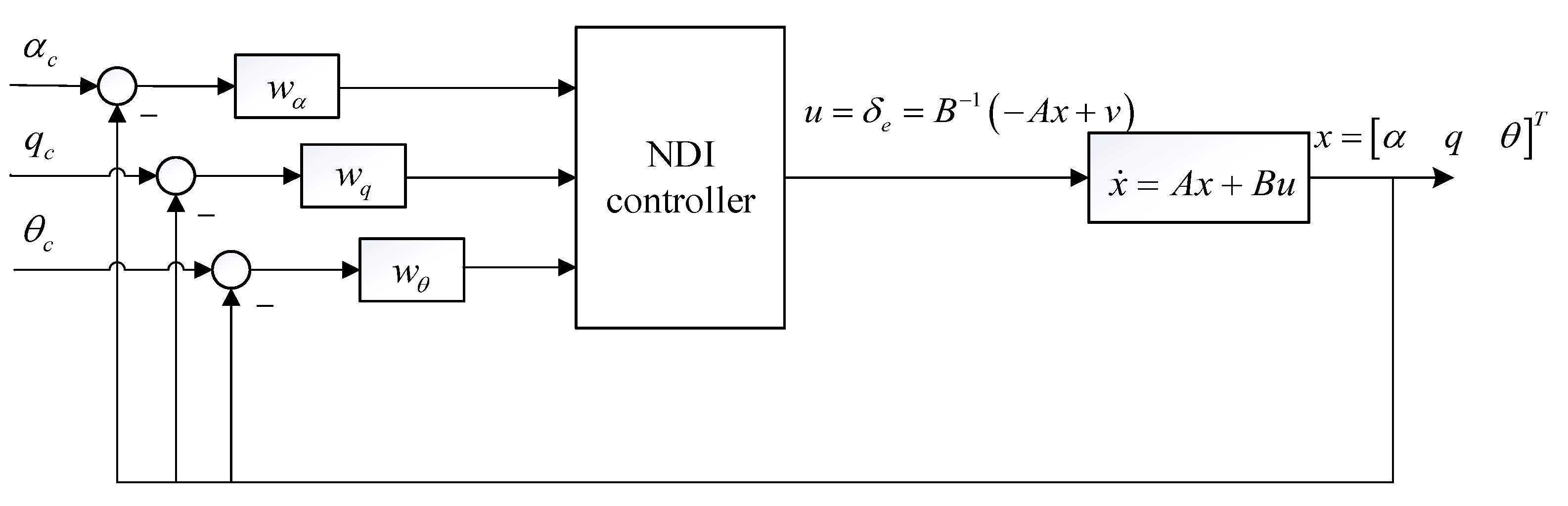
2.2. Nominal NDI Controller Design

During the HFV flight, in order to make the system state variable x = [α, q, θ]^T track the given command x_c = [α_c, q_c, θ_c]^T, a nominal NDI controller is designed according to Equation (1). When HFV has no inertia uncertainty, the nominal NDI controller is designed as follows:

$$u=B^{-1}(-Ax+v)$$

(15)

where v is the virtual controller, the design method is as follows:

$$v={\dot{x}}_c-Ke$$

(16)

where

$$e=x-x_c$$

(17)

Since the desired state quantity is usually constant, ${\dot{x}}_c$ is usually 0. K is the feedback gain matrix to be designed, the form is as follows:

$$K=\left[\begin{array}{ccc}{w}_{\alpha }& 0& 0\\ 0& w_q& 0\\ 0& 0& w_{\theta }\end{array}\right]$$

(18)

where w_α, w_q, w_θ represent the control loop bandwidth, and the values are 40 rad/s, 0.6 rad/s, and 40 rad/s, respectively. The test shows that the larger w_α, w_θ, the more severe the response curve oscillation; the smaller w_q, the more severe the response curve oscillation. The block diagram of the nominal NDI controller is shown in Figure 1.

3. Hybrid Compensation Scheme

This section mainly studies the design of an adaptive NDI controller for the HFV model with uncertain parameters of inertia to make the system closed-loop stable. In order to achieve the control objectives, the following problems need to be solved:

(1)

Considering the longitudinal two-degree-of-freedom small perturbation model, how to deal with the nonlinear term in the linearized system, and how to apply the nonlinear control method to design the nonlinear control law in the model;

(2)

Considering the parameter uncertainty of the moment of inertia in the system, how to design a suitable Lyapunov function for the state quantity and error of the system to obtain the adaptive law.

3.1. Adaptive NDI Controller for Inertia Uncertainty

Theoretically, the designed nominal NDI feedback controller (15) can make the aircraft track a given flight command, but in actual flight, the attitude angle and attitude angular velocity channels are easily affected by the external flight environment, which makes the aircraft have parameter uncertainty. The uncertainty of the moment of inertia is considered here, and it needs to be suppressed to improve the robustness of the flight control system. Model the drift characteristics of the aircraft’s moment of inertia parameters, and express the uncertainty of the moment of inertia in the following random form:

$$I_y=I_{y0}(1+\mathsf{\Delta }{I}_y)$$

(19)

where I_y represents the rotational inertia around the y-axis, I_y0 represents the nominal value of the parameter I_y, ΔI_y represents the increment of the parameter I_y, and its range is ǀΔI_yǀ ≤ I_y1, and I_y1 is positive.

In order to enhance the robustness of the system, an adaptive NDI controller is designed to make the aircraft immune to the uncertainty of the rotational inertia parameters, and the system output accurately tracks the given reference signal. The block diagram of the adaptive NDI controller is shown in Figure 2.

The adaptive NDI controller design process is as follows:

Consider the system reference model, that is, the model without uncertainty as follows:

$${\dot{x}}_m=A_m{x}_m+B_{m}u$$

(20)

The actual system model with rotational inertia uncertainty is as follows:

$${\dot{x}}_p=A_p(t)x_p+B_p(t)u$$

(21)

Based on the reference model, the designed nominal NDI control law (see Section 2.2 for the derivation process) is as follows:

$$u=g^{-1}(x)({\dot{x}}_c-Ke)$$

(22)

where $e=x-x_c$, K is the control bandwidth matrix.

The generalized error vector of the system is

$$e_1=x_m-x_p$$

(23)

and the equation with the generalized error as the state vector is

$${\dot{e}}_1=A_m{e}_1+[A_m-A_p(t)-B_p(t){\mathsf{\Theta }}_1(t)]x_p+[B_m-B_p(t){\mathsf{\Theta }}_2(t)]u$$

(24)

In order to make the dynamic response of the uncertain system (21) to the input u exactly the same as the dynamic response of the reference model (20) to the input u, the adaptive law adjusts Θ₁(t) and Θ₂(t) so that the uncertain system model matches the reference model, i.e.,

$$A_m=A_p(t)+B_p(t){\mathsf{\Theta }}_1{}^{*}$$

(25)

$$B_m=B_p(t){\mathsf{\Theta }}_2{}^{*}$$

(26)

The function with “*” represents the optimal state when the model is completely matched, and Equation (20) can be written as

$${\dot{e}}_1=A_m{e}_1+B_m{\mathsf{\Theta }}_2{}^{*-1}{\tilde{\mathsf{\Theta }}}_1{x}_p+B_m{\mathsf{\Theta }}_2{}^{*-1}{\tilde{\mathsf{\Theta }}}_{2}u$$

(27)

where the errors of the two adjustable functions are a 1 × 3-order matrix and a 1 × 1-order matrix, respectively, and satisfy

$${\tilde{\mathsf{\Theta }}}_1={{\mathsf{\Theta }}_1}^{*}-{\mathsf{\Theta }}_1$$

(28)

$${\tilde{\mathsf{\Theta }}}_2={{\mathsf{\Theta }}_2}^{*}-{\mathsf{\Theta }}_2$$

(29)

Theorem 1.

For the generalized error system (24), there is a Lyapunov function that contains the state error e₁ and the adjustable function errors (28) and (29). If there are dimensionally adjustable parameters P, R₁, and R₂ such that the derivative of the Lyapunov function satisfying the condition is less than zero, then the system (24) is stable.

Proof of Theorem 1.

The Lyapunov theory is used to design the adaptive laws, as shown below:

$$V=\frac{1}{2}{e}_1{}^{T}P{e}_1+\frac{1}{2}tr({\tilde{\mathsf{\Theta }}}_1^T{R}_1^{-1}{\tilde{\mathsf{\Theta }}}_1^T)+\frac{1}{2}tr({\tilde{\mathsf{\Theta }}}_2^T{R}_2^{-1}{\tilde{\mathsf{\Theta }}}_2^T)$$

(30)

where tr(·) represents the trace of the matrix, that is, the sum of the diagonal elements, and the Lyapunov function can be derived from time to obtain:

$$\begin{array}{l}\dot{V}=\frac{1}{2}{e}_1{}^T(P{A}_m+A_m^{T}P)e_1+tr({\dot{\tilde{\mathsf{\Theta }}}}_1^T{R}_1^{-1}{\tilde{\mathsf{\Theta }}}_1^T+x_p{e}_1{}^{T}P{B}_m{\mathsf{\Theta }}_2{}^{*-1}{\tilde{\mathsf{\Theta }}}_1)\\ \hspace{0.17em}\hspace{0.17em}\hspace{0.17em}\hspace{0.17em}\hspace{0.17em}+tr({\dot{\tilde{\mathsf{\Theta }}}}_2^T{R}_2^{-1}{\tilde{\mathsf{\Theta }}}_2^T+u{e}_1{}^{T}P{B}_m{\mathsf{\Theta }}_2{}^{*-1}{\tilde{\mathsf{\Theta }}}_2)\\ \hspace{0.17em}\hspace{0.17em}\hspace{0.17em}\le 0\end{array}$$

(31)

where P_3×3, R₁⁻¹_,3×3, R₂⁻¹_,1×1 is the positive definite symmetric matrix to be designed, and select P = diag(15, 2, 0), R₁ = diag(0.5, 0.5, 0.5), R₂ = 20. When debugging parameters, the larger R₁ is, the smaller the system oscillation is, but the slower the response speed is; the larger the R₂ is, the faster the system response speed is, but the oscillation will also increase.

For (31) to hold, the following conditions should be met:

$$A_m{}^{T}P+P{A}_m<0$$

(32)

To ensure that (31) is negative definite, the second and third terms are always 0, thence

$${\dot{\tilde{\mathsf{\Theta }}}}_1=-R_1(B_m{\mathsf{\Theta }}_2{}^{*-1})P{e}_1{x}_p{}^T$$

(33)

$${\dot{\tilde{\mathsf{\Theta }}}}_2=-R_2(B_m{\mathsf{\Theta }}_2{}^{*-1})P{e}_1{u}^T$$

(34)

where the adjustable parameter errors are

$$\{\begin{array}{l}{\tilde{\mathsf{\Theta }}}_1={{\mathsf{\Theta }}_1}^{*}-{\mathsf{\Theta }}_1\\ {\tilde{\mathsf{\Theta }}}_2={{\mathsf{\Theta }}_2}^{*}-{\mathsf{\Theta }}_2\end{array}$$

(35)

The adaptive parameter update law is designed as follows:

$${\dot{\mathsf{\Theta }}}_1=R_1(B_m{{\mathsf{\Theta }}_2}^{*-1})P{e}_1{x}_p{}^T$$

(36)

$${\dot{\mathsf{\Theta }}}_2=R_2(B_m{\mathsf{\Theta }}_2{}^{*-1})P{e}_1{u}^T$$

(37)

$${\mathsf{\Theta }}_1(t)={\displaystyle {\int }_0^t{R}_1(B_m{\mathsf{\Theta }}_2{}^{*-1})P{e}_1{x}_p{}^{T}dt+{\mathsf{\Theta }}_1(0)}$$

(38)

$${\mathsf{\Theta }}_2(t)={\displaystyle {\int }_0^t{R}_2(B_m{\mathsf{\Theta }}_2{}^{*-1})P{e}_1{u}^T}dt+{\mathsf{\Theta }}_2(0)$$

(39)

According to the above inequality (32) and the adaptive laws, Theorem 1 can be proved. Ultimately, the general system (24) is stable. □

In summary, when inertia uncertainty occurs, the passive adaptive NDI controller with multi-adaptive laws can directly compensate for the uncertainty and keep the high maneuvering HFV in stable flight.

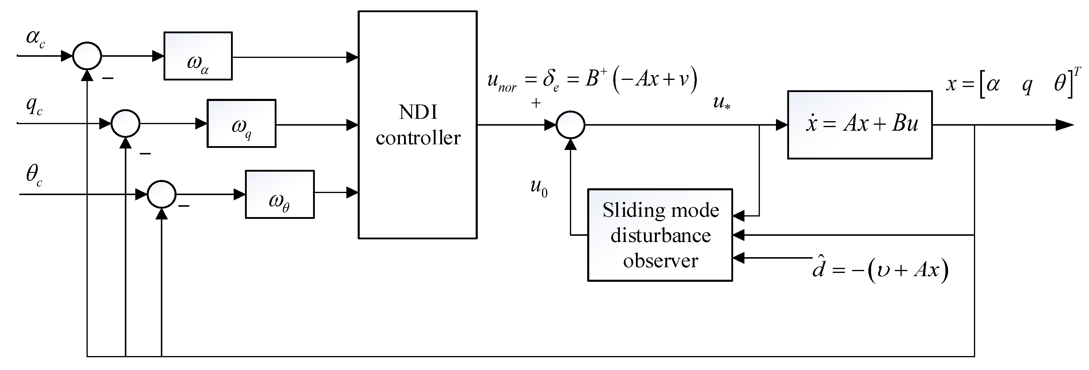
3.2. Active Sliding Mode NDI Controller for Disturbance

In order to optimize the control effect of the adaptive NDI controller, a sliding mode scheme is added here to improve the adaptive NDI controller and compensate for the influence of disturbance on the system. The nonlinear model of the aircraft under the influence of disturbance can be expressed as

$$\{\begin{array}{l}\dot{x}=Ax+Bu+d\\ y=Cx+Du\end{array}$$

(40)

d(t) in Formula (40) is the uncertain disturbance from external sources. According to the cancellation principle in NDI design, in the presence of disturbance and rotational inertia uncertainty, the nonlinear system control law is

$$u_{*}=B^{+}(-Ax+v-d)$$

(41)

The control u obtained by ignoring the disturbance solution is just an ideal flight control law. As d continues to increase, the system will slowly diverge and even become unstable. Aiming at this problem, a sliding mode disturbance observer is introduced to estimate the disturbance value, replacing d in (41), and then a new active compensation control law is used to repair the disturbance.

The block diagram of the sliding mode NDI controller is shown in Figure 3.

For the MIMO nonlinear uncertain system (40), construct the following sliding mode system with a disturbance observer:

$$\{\begin{array}{l}s=x-z\\ \dot{z}=Bu-\upsilon \\ \widehat{d}=-(\upsilon +Ax)\end{array}$$

(42)

where s = [s₁, s₂, s₃]^T is the auxiliary sliding mode surface, and the sliding mode control variable is

$$\upsilon ={[\begin{array}{ccc}{\upsilon }_1& {\upsilon }_2& {\upsilon }_3\end{array}]}^T=-\varphi sign(s)$$

(43)

and

$$sign(s)={[\begin{array}{ccc}sign(s_1)& sign(s_2)& sign(s_3)\end{array}]}^T$$

(44)

$$\varphi =diag({\varphi }_1,{\varphi }_2,{\varphi }_3)$$

(45)

thence υ can be expressed as (46), i = 1, 2, 3,

$${\upsilon }_i=-{\varphi }_{i}sign(s_i)$$

(46)

$$\upsilon ={\left[\begin{array}{ccc}-{\upsilon }_{1}sign(s_1)& -{\upsilon }_{2}sign(s_2)& -{\upsilon }_{3}sign(s_3)\end{array}\right]}^T$$

(47)

Let

$$\xi =Ax+\widehat{d}={[\begin{array}{ccc}{\xi }_1& {\xi }_2& {\xi }_3\end{array}]}^T$$

(48)

when ${\varphi }_i>\left|{\xi }_i\right|$, the observation of disturbance $\widehat{d}$ can uniformly converge asymptotically to the true value.

Taking the derivation of the first formula of (42):

$$\begin{array}{l}\dot{s}=\dot{x}-\dot{z}\\ \hspace{0.17em}\hspace{0.17em}=Ax+Bu+d-Bu+\upsilon \\ \hspace{0.17em}\hspace{0.17em}=Ax+d+\upsilon \end{array}$$

(49)

Theorem 2.

If the algorithms (43)~(47) designed for the system (42) satisfy the condition (50), the sliding mode dynamic system (42) is uniformly stable.

$$\{\begin{array}{l}{\upsilon }_i=-{\varphi }_{i}sign(s_i)\\ {\varphi }_i>\left|{\xi }_i\right|\end{array}$$

(50)

Proof of Theorem 2.

Take the Lyapunov function

$$V=\frac{1}{2}{s}^{T}s\ge 0$$

(51)

Then

$$\begin{array}{l}\dot{V}=s^T\dot{s}\\ \hspace{0.17em}\hspace{0.17em}\hspace{0.17em}={\displaystyle \sum _{i=1}^3{s}_i}{\dot{s}}_i\\ \hspace{0.17em}\hspace{0.17em}\hspace{0.17em}={\displaystyle \sum _{i=1}^3{s}_i}({\xi }_i+v_i)\end{array}$$

(52)

Define

$${\dot{V}}_i=s_i({\xi }_i+v_i)$$

(53)

because (50), we can obtain:

$$\begin{array}{l}{\dot{V}}_i=s_i({\xi }_i+v_i)\\ \hspace{0.17em}\hspace{0.17em}\hspace{0.17em}=s_i{\xi }_i-s_i{\varphi }_{i}sign(s_i)\\ \hspace{0.17em}\hspace{0.17em}\hspace{0.17em}\le s_i\left|{\xi }_i\right|-s_i{\varphi }_{i}sign(s_i)\hspace{0.17em}\\ \hspace{0.17em}\hspace{0.17em}\hspace{0.17em}<s_i{\varphi }_i-s_i{\varphi }_{i}sign(s_i)\\ \hspace{0.17em}\hspace{0.17em}\hspace{0.17em}=\{\begin{array}{l}0,s_i\ge 0\\ 2s_i{\varphi }_i<0,s_i<0\end{array}\end{array}$$

(54)

Then we can obtain

$$\{\begin{array}{l}{\dot{V}}_i<0\\ \dot{V}={\displaystyle \sum _{i=1}^3{\dot{V}}_i}<0\end{array}$$

(55)

Therefore, s is stable in the equilibrium state at the origin, satisfying the stability condition. □

When the system reaches a stable point, it can be known from Equations (40)–(42) that the observed disturbance value is

$$\widehat{d}=-(\upsilon +Ax)$$

(56)

Since υ is a switching function, there will be a lot of chattering during simulation, which will affect the tracking performance. Therefore, the relatively smooth hyperbolic tangent function tanh(s) is used to replace the switching term sign(s) to reduce the chattering.

The disturbance compensation law is designed as

$$u_o=-B^{+}\widehat{d}$$

(57)

Finally, the adaptive sliding mode NDI controller is:

$$\begin{array}{l}{u}_{*}=u_{nor}+u_o\\ \hspace{0.17em}\hspace{0.17em}\hspace{0.17em}=B^{+}(-Ax+v)-B^{+}\widehat{d}\\ \hspace{0.17em}\hspace{0.17em}\hspace{0.17em}=B^{+}(v-Ax-\widehat{d})\end{array}$$

(58)

Combining the adaptive control law with the sliding mode control law, the block diagram of the adaptive sliding mode NDI controller is shown in Figure 4.

Remark 3.

In engineering, the fast response of HFV needs a high-performance computer on a missile, which is not to solve a certain problem, but to create conditions for all the fast response needs. Our hardware is advanced enough to adapt the chattering signal with only the ultra-fast computational power of the missile-based high-performance computer and to transmit this signal in time to the composite adaptive laws designed in this study. Furthermore, any slight chattering under sea-skimming conditions can be promptly compensated by the supercomputer and the adaptive algorithm.

4. Simulation Results and Analysis

In this section, simulation experiments and result analysis are used to verify the effectiveness of the designed NDI controller to ensure that the system can track the given command. Figure 5 is the LINK-BOX semi-physical simulation platform. Links-Box automatically converts the MATLAB simulation models to the embedded control prototype and supports engineering hardware to test the models. The physical device can be directly connected to the rapid prototyping simulator to dynamically verify controller performance. The features of the software package Links-RT are: (1) adapting to the models built in MATLAB; (2) providing input and output hardware to enable users to integrate the hardware environment into the simulation models; (3) automatic conversion of MATLAB model codes to VxWorks codes.

The simulation conditions and partial control parameters are shown in

Table 2. HFV simulation control parameters.

Parameter Meaning	Symbol	Parameter Value
HFV mass	m	9295.44 kg
Pitch moment of inertia	Iy	75,673.8 kg·m2
Reference wing area	S	28.87 m2
Span	b	9.144 m2
Air density	ρ	1.22 kg/m3
Flight speed	V	5104.41 m/s
Track inclination angle	μ	0 deg (°)
Acceleration due to gravity	g	9.806 m/s2

. The simulation time is 20 s.

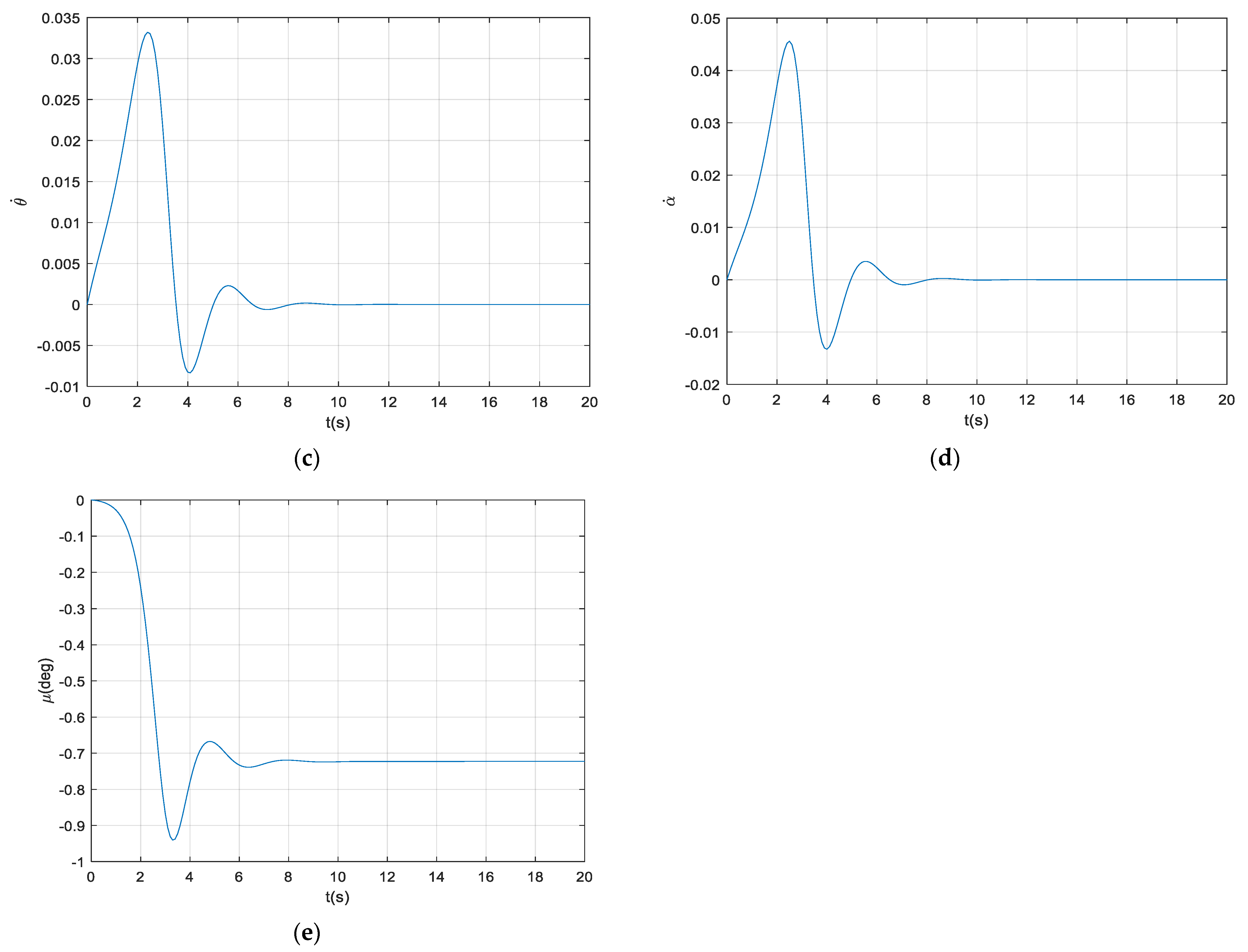
4.1. Nominal NDI Controller Simulation

The normal overload Nys of HFV is expressed as

$$Nys=\frac{V}{g}(q-\dot{\alpha })+\frac{I_{xs}}{g}\dot{q}$$

(59)

where I_xs is the distance from the center of gravity of the aircraft to the normal overload sensor. The track inclination of the aircraft is expressed as

$$\mu =\theta -\alpha$$

(60)

The small disturbance linearization processing method must be used near a certain system equilibrium point, and the equilibrium state is selected as the angle of attack α₀ = 3.25 deg.

Set the reference signals to

$${\alpha }_c=4\times \frac{\pi }{180}rad,q_c=0rad/s,{\theta }_c=3.27\times \frac{\pi }{180}rad$$

the simulation initial conditions are α = 0 rad, q = 0 rad/s, θ = 0 rad.

The simulation results of the nominal controller are shown in Figure 6.

The simulation results show that the system can quickly recover to a stable state, and the system state x = [α, q, θ]^T can track the given reference command x_c = [α_c, q_c, θ_c]^T, the derivative of the state variable can eventually tend to 0, and the normal overload Nys tends to 0, which satisfies the control objective. When the system moves longitudinally, the default sideslip angle β = 0, and the selected equilibrium state should ensure that the track inclination angle μ = 0. The simulation results show that the track inclination angle μ is finally stabilized at −0.72 deg, which is slightly different from the ideal state. There is still room for improvement in compensating for parameter perturbation.

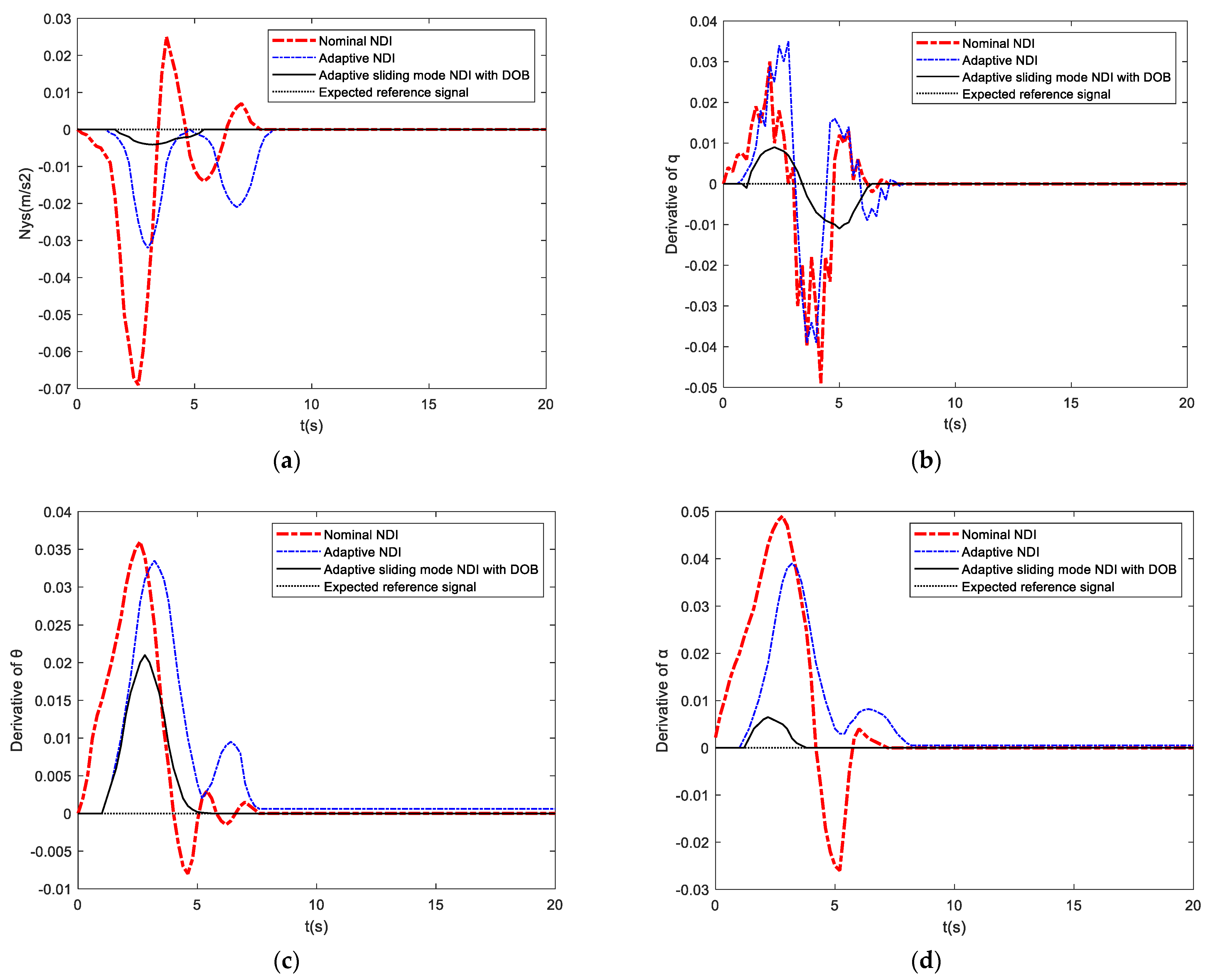
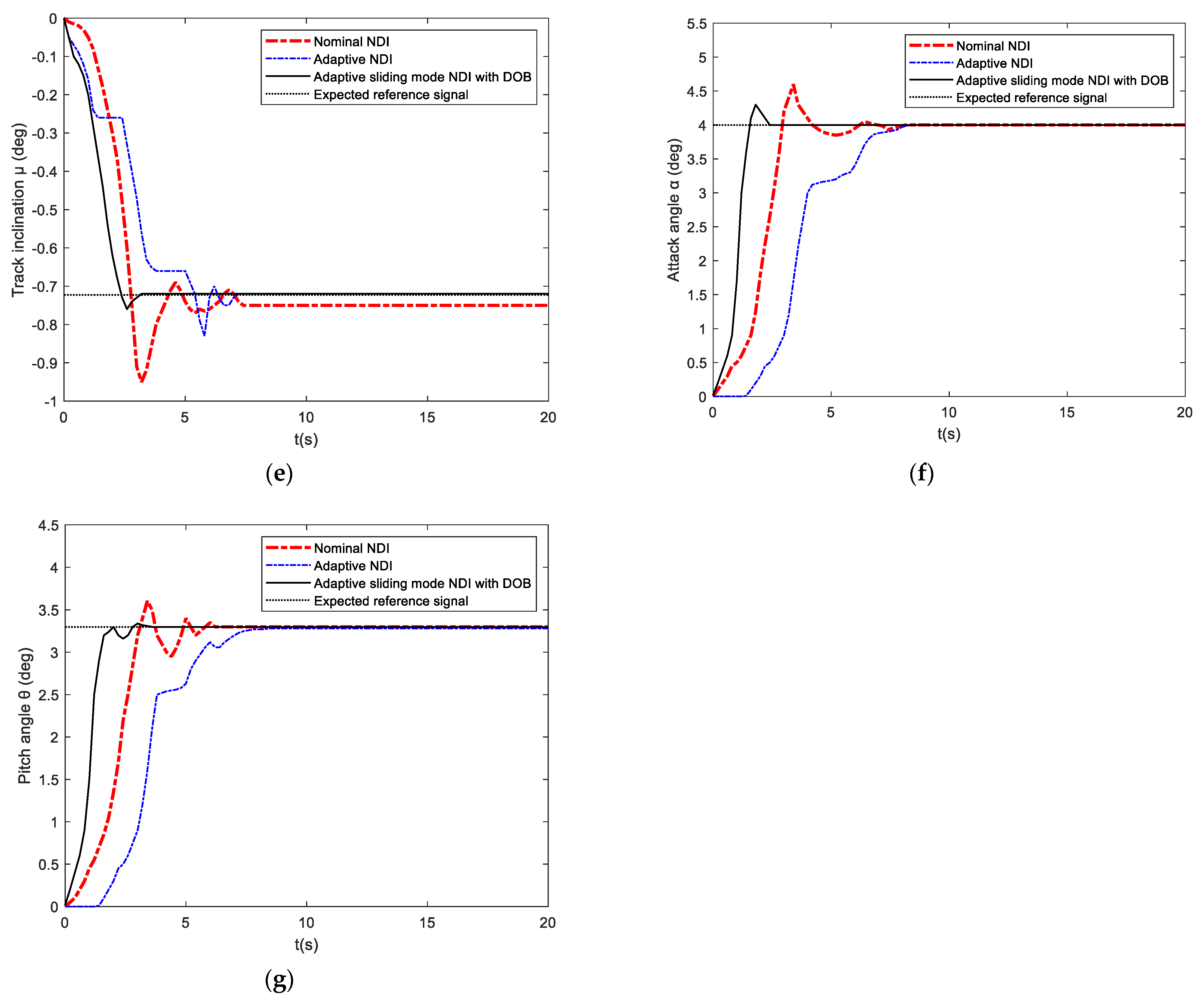
4.2. Hybrid Adaptive Compensation Simulation of Sliding Mode NDI

Set the reference signal as

$$\{\begin{array}{l}{\alpha }_c=4\times \frac{\pi }{180}rad\\ q_c=0rad/s\\ {\theta }_c=3.27\times \frac{\pi }{180}rad\end{array}$$

the initial condition as α = 0 rad, q = 0 rad/s, θ = 0 rad. The uncertainty mainly affects the aerodynamic parameters $M_z^{\alpha }$, $M_z^{{\delta }_e}$, $M_z^{\dot{\alpha }}$, $M_z^q$, from the state matrix A, B, C, and D of the system, it can be known that these four aerodynamic parameters mainly affect the pitch rate channel and the system output $\dot{q}$, thereby indirectly affecting the normal overload. Therefore, the influence of uncertainty on the system is mainly manifested in the change in pitch angle and speed. Here, the uncertainty range is enlarged to ±20%, and the uncertainty of the pitch moment of inertia I_y takes the following form:

$$I_y=I_{y0}(1+\mathsf{\Delta }{I}_y(2rand(1,1)-1))$$

(61)

The compound disturbance settings are as follows:

$$d={[0.05sin(0.1t), 0.1sint, 0.1sin(10t)]}^T$$

(62)

In the proposed adaptive sliding mode controller, select P = diag(15, 2, 0), R₁ = diag(0.5, 0.5, 0.5), R₂ = 20. Due to high-level military secrecy, only a part of the controller parameters is presented in this study.

The simulation results of NDI control, adaptive NDI control, and adaptive sliding mode NDI control are compared for the longitudinal system with ±20% moment of inertia uncertainty and are shown in Figure 7, where “DOB” means the disturbance observer.

From Figure 7, it can be seen that when the system has inertia uncertainty and elastic modal disturbance, the adaptive NDI controller can reduce the oscillation of each channel. The improved adaptive sliding mode NDI controller can more obviously suppress the oscillation of the attitude angle and angular velocity channels, effectively compensate for the disturbance and uncertain parameters of inertia, and ensure the stability and tracking performance of the HFV.

Table 3. Comparative analysis I of performance indicators between proposed algorithms.

	Nominal NDI	Adaptive NDI	Adaptive Sliding Mode NDI
ts,max	7.95	7.99	5.28
ts,min	5.01	5.10	1.61
ess,max	0.03	0.001	0.0004
ess,min	0.0003	0.0002	0.0001
ov,max	30.56%	13.89%	7.50%
ov,min	18.18%	0.005%	0.03%

is the tracking performance table based on the statistics of Figure 6. In view of the general definition of overshoot, only Figure 6e–g has overshoot [30]. The three controllers in the table represent the three stages of improving NDI in this paper: nominal, adaptive, and adaptive sliding mode.

The shortest response time (t_s,min) of the hybrid compensation NDI, that is, the adaptive sliding mode controller, is only 32% of the nominal controller, the maximum steady-state error (e_ss,max) is only 1% of the nominal controller, the overshoot (o_v,max) is only 24% of the nominal controller. Other indicators have also been greatly improved, so the active–passive hybrid compensation NDI is more suitable for high maneuvering HFV.

Table 4. Comparative analysis II of performance indicators between ideal and harsh models.

	HFV without Uncertainty, Disturbance, and Model Error	HFV in This Paper
ts,max	5.15	5.28
ts,min	2.51	1.61
ess,max	0.0003	0.0004
ess,min	0.0001	0.0001
ov,max	3.96%	7.50%
ov,min	0.001%	0.03%

shows the performance comparison result of the proposed method in the HFV model without disturbance, uncertain parameters, and modeling error and the HFV model in this paper. To ensure the fairness of the comparison, the proposed finished algorithm is used in both models.

Table 4 shows that the proposed method can also adapt to normal non-severe flight conditions. The only drawback is the response time, as the complex algorithm slows down the HFV response, resulting in a minimum response time of about 1 s. Other performance indicators are better than the harsh environment considered in this paper.

Table 5. Comparative analysis III of performance between method in [5] and proposed method.

	State-of-Art Method	Proposed Method
ts,max	27.27	5.28
ts,min	10.01	1.61
ess,max	12.29	0.0004
ess,min	1.3	0.0001
ov,max	166.76%	7.50%
ov,min	38.63%	0.03%

shows the comparative analysis result of the proposed method and the existing state-of-art method in reference [5]. To ensure fairness, the controlled object is set to the longitudinal HFV model.

Simulation result shows that the maximum response time of the existing method is beyond the simulation time interval [0, 20s] allowed by the experiment, so it cannot meet the requirements of HFV flight simulation in a real environment. The time of the proposed method is reduced by 18% of the existing method, and the steady-state errors are compressed by more than 10,000 times, which greatly improves the performance of HFV under the co-existence of multiple uncertainties in sea-skimming flight, and has obvious advantages.

5. Conclusions

The hybrid compensation method demonstrated in this study keeps HFV stable under the concurrent conditions of multi-uncertain factors. The nominal NDI compensates for the modeling error of the longitudinal model using direct subtraction of corresponding terms. Based on multi-adaptive laws, the adaptive NDI controller compensates for the inertia uncertainties, so that the HFV maintains attitude stability under high maneuvering conditions. Furthermore, a disturbance observer helps the improved sliding mode adaptive NDI controller to estimate and actively repair the disturbance. Finally, the hybrid strategy enables the HFV to regain attitude stability with passive and active compensation methods, respectively, in the face of uncertain inertia and disturbance. The proposed method solves the multi-source uncertain robust control problem of the HFV. The subsequent research direction is automatic multi-fault repair.

References

1. Han, T.; Hu, Q.; Shin, H.; Tsourdos, A.; Xin, M. Incremental twisting fault tolerant control for hypersonic vehicles with partial model knowledge. IEEE Trans. Ind. Inform. 2022, 18, 1050–1060. [Google Scholar] [CrossRef]
2. Xu, B.; Shi, Z.; Sun, F.; He, W. Barrier lyapunov function based learning control of hypersonic flight vehicle with AOA constraint and actuator faults. IEEE Trans. Cybern. 2019, 49, 1047–1057. [Google Scholar] [CrossRef] [PubMed]
3. Wang, Y.; Yang, X.; Yan, H. Reliable fuzzy tracking control of near-space hypersonic vehicle using aperiodic measurement information. IEEE Trans. Ind. Electron. 2019, 66, 9439–9447. [Google Scholar] [CrossRef]
4. Bu, X.; Xiao, Y.; Lei, H. An adaptive critic design-based fuzzy neural controller for hypersonic vehicles: Predefined behavioral nonaffine control. IEEE/ASME Trans. Mechatron. 2019, 24, 1871–1881. [Google Scholar] [CrossRef]
5. Sun, J.; Yi, J.; Pu, Z.; Tan, X. Fixed-time sliding mode disturbance observer-based nonsmooth backstepping control for hypersonic vehicles. IEEE Trans. Syst. Man Cybern. Syst. 2020, 50, 4377–5386. [Google Scholar] [CrossRef]
6. Ren, W.; Jiang, B.; Yang, H. Singular perturbation-based fault-tolerant control of the air-breathing hypersonic vehicle. IEEE ASME Trans. Mechatron. 2019, 24, 2562–2571. [Google Scholar] [CrossRef]
7. Li, F.; Xiong, J.; Lan, X.; Bi, H.; Chen, X. NSHV trajectory prediction algorithm based on aerodynamic acceleration EMD decomposition. J. Syst. Eng. Electron. 2021, 32, 103–117. [Google Scholar]
8. Sun, J.; Yi, J.; Pu, Z.; Liu, Z. Adaptive fuzzy nonsmooth backstepping output-feedback control for hypersonic vehicles with finite-time convergence. IEEE Trans. Fuzzy Syst. 2020, 28, 2320–2334. [Google Scholar] [CrossRef]
9. Yang, G.; Yao, J.; Nasim, U. Neuroadaptive control of saturated nonlinear systems with disturbance compensation. ISA Trans. 2022, 122, 49–62. [Google Scholar] [CrossRef]
10. Yang, G.; Yao, J.; Dong, Z. Neuroadaptive learning algorithm for constrained nonlinear systems with disturbance rejection. Int. J. Robust Nonlinear Control 2022, 32, 6127–6147. [Google Scholar] [CrossRef]
11. Guo, Z.; Guo, J.; Zhou, J.; Chang, J. Robust tracking for hypersonic reentry vehicles via disturbance estimation-triggered control. IEEE Trans. Aerosp. Electron. Syst. 2020, 56, 1279–1289. [Google Scholar] [CrossRef]
12. Hu, Y.; Geng, Y.; Wu, B.; Wang, D. Model-free prescribed performance control for spacecraft attitude tracking. IEEE Trans. Control Syst. Technol. 2021, 29, 165–179. [Google Scholar] [CrossRef]
13. Sun, J.; Pu, Z.; Yi, J.; Liu, Z. Fixed-time control with uncertainty and measurement noise suppression for hypersonic vehicles via augmented sliding mode observers. IEEE Trans. Ind. Inform. 2020, 16, 1192–1203. [Google Scholar] [CrossRef]
14. Mu, C.; Ni, Z.; Sun, C.; He, H. Air-breathing hypersonic vehicle tracking control based on adaptive dynamic programming. IEEE Trans. Neural Netw. Learn. Syst. 2017, 28, 584–598. [Google Scholar] [CrossRef]
15. Zhang, M.; Ali, N.; Gao, Q. Winding inductance and performance prediction of a switched reluctance motor with an exterior-rotor considering the magnetic saturation. CES Trans. Electr. Mach. Syst. 2021, 5, 212–223. [Google Scholar] [CrossRef]
16. Ma, G.; Chen, C.; Lyu, Y.; Guo, Y. Adaptive backstepping-based neural network control for hypersonic reentry vehicle with input constraints. IEEE Access 2018, 6, 1954–1966. [Google Scholar] [CrossRef]
17. Chen, L.; Wang, Q.; Ye, H.; He, G. Low-complexity adaptive tracking control for unknown pure feedback nonlinear systems with multiple constraints. IEEE Access 2019, 7, 27615–27627. [Google Scholar] [CrossRef]
18. Meng, F.; Tian, K.; Wu, C. Deep reinforcement learning-based radar network target assignment. IEEE Sens. J. 2021, 21, 16315–16327. [Google Scholar] [CrossRef]
19. An, H.; Liu, J.; Wang, C.; Wu, L. Disturbance observer-based antiwindup control for air-breathing hypersonic vehicles. IEEE Trans. Ind. Electron. 2016, 63, 3038–3049. [Google Scholar] [CrossRef]
20. Yu, X.; Li, P.; Zhang, Y. Fixed-time actuator fault accommodation applied to hypersonic gliding vehicles. IEEE Trans. Autom. Sci. Eng. 2021, 18, 1429–1440. [Google Scholar] [CrossRef]
21. Gao, K.; Song, J.; Wang, X.; Li, H. Fractional-order proportional-integral-derivative linear active disturbance rejection control design and parameter optimization for hypersonic vehicles with actuator faults. Tsinghua Sci. Technol. 2021, 26, 9–23. [Google Scholar] [CrossRef]
22. Cui, B.; Xia, Y.; Liu, K.; Zhang, J.; Wang, Y.; Shen, G. Truly distributed finite-time attitude formation-containment control for networked uncertain rigid spacecraft. IEEE Trans. Cybern. 2022, 52, 5882–5896. [Google Scholar] [CrossRef] [PubMed]
23. Ai, S.; Song, J.; Cai, G. Diagnosis of sensor faults in hypersonic vehicles using wavelet packet translation based support vector regressive classifier. IEEE Trans. Reliab. 2021, 70, 901–915. [Google Scholar] [CrossRef]
24. Li, J.; Chen, S.; Li, C.; Wang, F. Distributed game strategy for formation flying of multiple spacecraft with disturbance rejection. IEEE Trans. Aerosp. Electron. Syst. 2021, 57, 119–128. [Google Scholar] [CrossRef]
25. Li, Y. Finite time command filtered adaptive fault tolerant control for a class of uncertain nonlinear systems. Automatica 2019, 106, 117–123. [Google Scholar] [CrossRef]
26. Hu, K.; Li, W.; Cheng, Z. Fuzzy adaptive fault diagnosis and compensation for variable structure hypersonic vehicle with multiple faults. PLoS ONE 2021, 16, e0256200. [Google Scholar] [CrossRef] [PubMed]
27. Hu, K.; Chen, F.; Cheng, Z. Fuzzy adaptive hybrid compensation for compound faults of hypersonic flight vehicle. Int. J. Control Autom. Syst. 2021, 19, 2269–2283. [Google Scholar] [CrossRef]
28. Du, Y.; Jiang, B.; Ma, Y.; Cheng, Y. Robust ADP-based sliding-mode fault-tolerant control for nonlinear systems with application to spacecraft. Appl. Sci. 2022, 12, 1673. [Google Scholar] [CrossRef]
29. Xiao, B.; Hu, Q.; Wang, D.; Eng, K. Attitude tracking control of rigid spacecraft with actuator misalignment and fault. IEEE Trans. Control Syst. Technol. 2013, 21, 2360–2366. [Google Scholar] [CrossRef]
30. Su, J.; Chen, W. Model-based fault diagnosis system verification using reachability analysis. IEEE Trans. Syst. Man Cybern. Syst. 2019, 49, 742–751. [Google Scholar] [CrossRef] [Green Version]
Figure 1. Longitudinal HFV nominal NDI control scheme.
Applsci 12 11032 g001
Figure 2. Adaptive NDI control structure diagram of longitudinal HFV model.
Applsci 12 11032 g002
Figure 3. Longitudinal HFV model sliding mode NDI controller.
Applsci 12 11032 g003
Figure 4. Overall diagram of longitudinal HFV model adaptive sliding mode NDI control.
Applsci 12 11032 g004
Figure 5. Semi-physical simulation platform.
Applsci 12 11032 g005
Figure 6. Nominal NDI for HFV under modeling error. (a) Tracking curve of the normal overload Nys. (b) Tracking curve of pitch rate derivative q ˙ . (c) Tracking curve of the pitch derivative θ ˙ . (d) Tracking curve of the attack angle derivative α ˙ . (e) Tracking curve of the track inclination μ.
Applsci 12 11032 g006aApplsci 12 11032 g006b
Figure 7. Comparison of the effects of different HFV controllers under inertia uncertainty and disturbance. (a) Tracking curves of the normal overload Nys. (b) Tracking curves of pitch rate derivative q ˙ . (c) Tracking curves of the pitch derivative θ ˙ . (d) Tracking curves of the attack angle derivative α ˙ . (e) Tracking curves of the track inclination μ. (f) Tracking curves of the attack angle α. (g) Tracking curves of the pitch angle θ.
Applsci 12 11032 g007aApplsci 12 11032 g007b