The Interference Effects of Wind Load and Wind-Induced Dynamic Response of Quayside Container Cranes

Abstract

Strong wind has caused damage to group-arranged quayside container cranes in terminals and ports in recent years. Interference may amplify the wind loads in some cases. However, the interference effect among cranes has rarely been studied. In this study, high-frequency force balance tests were conducted to obtain the wind load of isolated and group-arranged container cranes. The results of the computational fluid dynamics simulation were validated by wind tunnel tests and provided the mean wind loads of all 15 types of member cranes. According to the results from wind tunnel tests, the fluctuating wind loads of each member were generated using the weighted amplitude wave superposition method. Based on dynamic finite element methods, the wind-induced responses were obtained considering the interference effect. It was found that the interference effect is the combined effects of both the shielding effect and the amplification of turbulence. Although in some cases the fluctuating and peak wind loads can increase by up to 16% and 6%, respectively, those in the most unfavorable cases are reduced by the interference effect. The interference factor for extreme nodal deformation is 0.56 and 0.69. The interference effect in container cranes mainly appears as a shielding effect, reducing the wind loads and response of the structures in unfavorable cases.

1. Introduction

In ports and terminals, quayside container cranes are used to transfer containers to and from ships and thus play an important role in cargo transportation. Given the significant growth in global trade along with rapid containerization and automation, mega quayside container cranes with an outreach of 65~70 m or more are common now. For such large dimensions, wind-related damage poses a severe threat to quayside container cranes [1]. Sixteen cranes in the Zhanjiang port in China suffered severe damage during a typhoon in 1999 [2]. At the Busan port in Korea, eight cranes designed according to the BS 2573-1 [3] code were severely damaged due to a typhoon, resulting in a loss of US$31 million [4]. The collapse of a single crane might initiate cascading failure events involving many nearby cranes and result in severe damage or even the collapse of multiple cranes [5,6,7,8]. Therefore, the wind-induced dynamic response should be carefully estimated to verify the stability and safety of the whole structure or the elements. In addition, the wind resistance of the cranes should be assessed.

To simplify the design procedure, the wind load is always considered as a static load without adjacent structures. It is found in many codes, such as British Standard, BS 2573-1 [3], American Society of Civil Engineers, ASCE 7-16 [9], European Standard, Eurocode 1-4 [10], Chinese standard, GB/T 3811-2008 [11] and Japanese standard [12]. In relevant studies on the impact of wind load on quayside container cranes, wind tunnel tests and CFD simulations were conducted (Gu, Huang & Wang [13], Han & Han [14], Huang, Wang, & Gu [15], Kang & Lee [16], Lee & Kang [17]). Xiao et al. [18] proposed a method to estimate the spatial distribution of wind loads on latticed towers and validated the method by performing wind tunnel tests. These studies mainly focused on the wind load and static wind-induced responses on the isolated crane, with no special consideration for exposure or shelter.

The wind load, especially the fluctuating component, cannot be ignored in both the kinetic and dynamic characteristics of the quayside cranes. Takahashi et al. [19] analyzed the dynamic runaway characteristics of quayside container cranes subjected to transient gusty winds and proposed the sliding state while approaching runaway and after runaway caused by a wind gust. Su et al. [20] studied the effect of stochastic dynamic transient gusty winds on the sliding and overturning of quayside container cranes and stated that dynamic transient gusty wind-induced peak response follows type III (Weibull) extreme value distribution. The above-mentioned studies employed wind loads and wind velocities according to the quasi-stationary assumption but ignored the spatial distribution of the wind loads. Sourav and Samit [4] analyzed the dynamic wind effect of quayside container cranes in stationary and nonstationary wind fields and noted that the failure vulnerability might not be the maximum for the set of parameter values for which the aerodynamic forces are maximum. Chen and Li [21] obtained the displacement of the latticed tower from nonlinear dynamic analysis. The result shows the displacements values obtained from time history analysis to be 5–28% higher than static displacements. Ziad et al. [22] conducted an aeroelastic lattice tower model in the wind tunnel test. The result shows that the resonance contribution is shown to reach a maximum of 18% of the peak response of the tower.

The wind-induced interference effect (IE) provides information regarding how an engineering structure reacts to changing forces or surface pressure in the presence of surrounding structures under wind loads. The interference effect has been studied for various structures, such as scaffoldings [23], cooling towers [24,25], tall buildings [26], and low-rise buildings [27,28,29,30] with different roof types. However, studies on the interference effect in quayside container cranes are rarely found. Other studies of lattice towers focus on the influence of antennas (Holmes et al. [31], Célio et al. [32], Patricia et al. [33]). The interference factor of microwave antenna dishes was found to be greater than one for some wind directions. This factor also depends on the solidity of the tower. However, studies on the interference effect among structures are scant.

Based on the literature, the present study focused on the interference effect on the wind loads and dynamic response among quayside cranes. High-frequency force balance tests (HFFB) were carried out in the wind tunnel to obtain the aerodynamic characteristic of the whole structure. The tests considered different wind yaw angles, structure states, and spacing to analyze the influence of IE on wind loads. Meanwhile, computational fluid dynamics (CFD) was performed to analyze the wind fields in detail, and the drag coefficients of each member were obtained as well. Based on these results, a randomly generated wind time history was used to model the wind loads considering the interference effect using the weighted amplitude wave superposition (WAWS) method. Numerical models for the quayside cranes were built in the commercial software ANSYS and the transient analysis was conducted using the finite element method (FEM). Then, the interference effect on wind-induced response was discussed. Finally, some brief conclusions were drawn and potential improvements for risk reduction for quayside cranes under strong wind were proposed.

2. The Procedure for the Analysis of the Interference Effects

Figure 1 shows the process of the wind-induced response analysis. To investigate the influence of IE on the wind load, both isolated models and group-arranged models were considered in the wind tunnel tests. The base shear force and moment were measured in the high-frequency force tests. The aerodynamic coefficients were obtained, and the fluctuating wind loads were analyzed. However, the wind tunnel test can only provide the wind load of the whole structure. Thus, CFD simulations were performed for the same cases to obtain the mean wind force of each member. Meanwhile, the wind field characteristics were investigated to seek the root cause of IE. Then, the fluctuating wind force time history of each member was determined based on the base moment spectrum by using the weighted amplitude wave superposition (WAWS) method. The wind-induced response was calculated using the finite element method (FEM). The influence of IE on the dynamic response was compared between isolated and group-arranged cranes. Finally, conclusions were summarized and some suggestions for wind prevention were provided.

3. Determination of the Wind Load

3.1. Wind Tunnel Tests

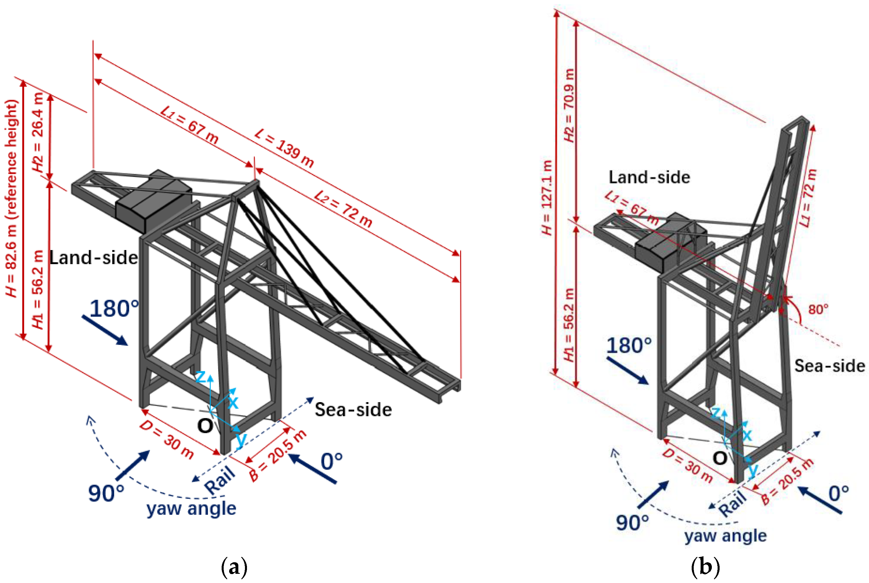
To obtain the aerodynamic force data for quayside container cranes, wind tunnel tests were conducted on rigid models. A 65T-65M container crane with a weight of 1380 t was applied as the prototype as it is the most widely used type among ports and terminals. The crane has a rated lifting capacity of 65 t and a lifting height of 65 m. The geometric characteristics of the container crane model and coordinate system are displayed in Figure 2. Both boom-down and boom-up positions were considered in the tests. 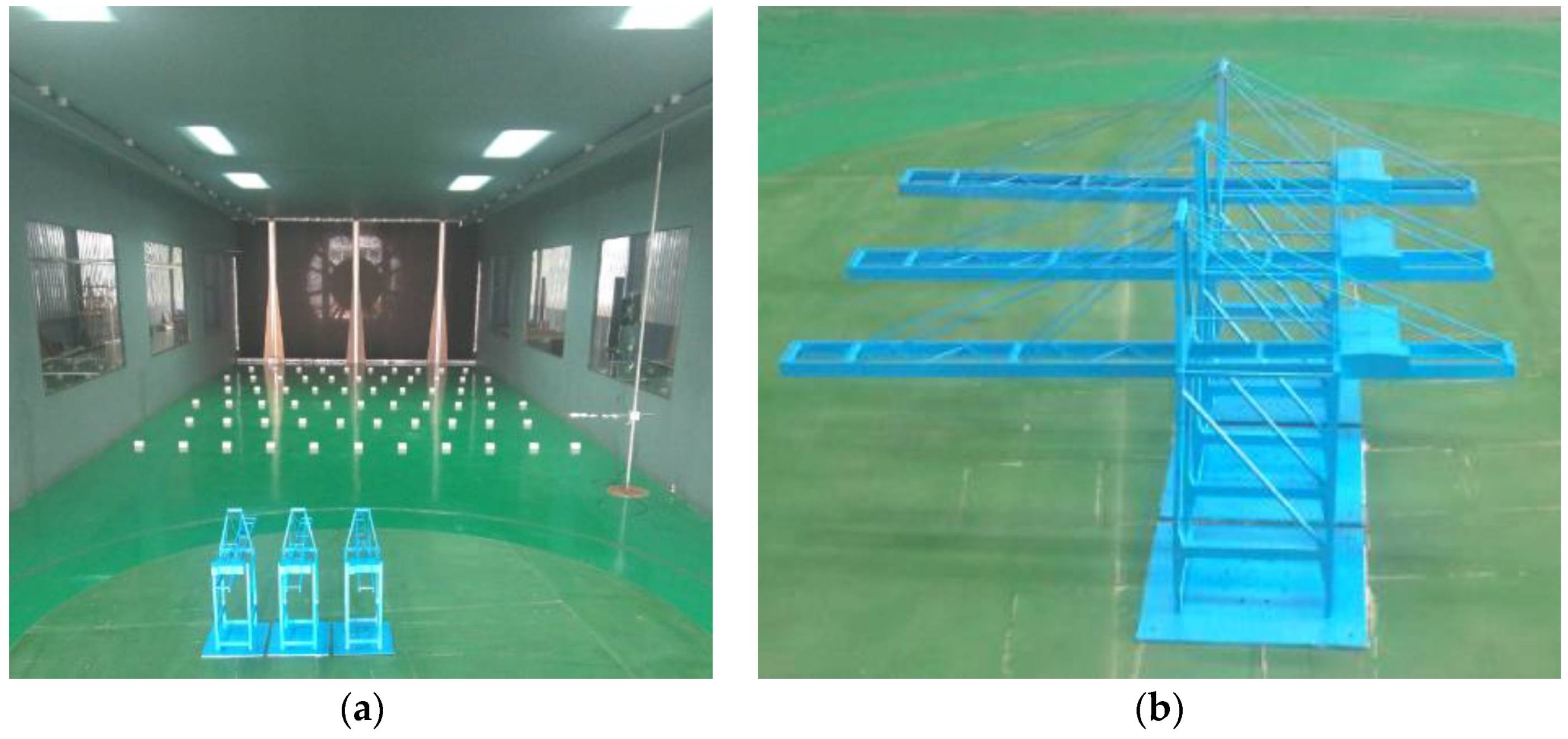Rigid models (Figure 3) with a geometric scale of 1:150 were fabricated for the wind tunnel tests with a maximum blockage ratio of 2.7%. There are two boom positions for the crane. The boom is horizontal as a boom-down state when lifting and loading containers. The non-working resting elevation angle of 80° was set in the boom-up state when resting or suffering from windstorms or other extreme weather. Aiming to model the actual arrangement pattern in ports, three models with the same size for both boom-up and boom-down positions were provided. The measured models were made of steel with welded joints so that the models were rigid enough to avoid aeroelastic effects and fluid-structure coupling.

The balance was fixed under the center of the turn table, sharing the same position with the measured model. Figure 3 shows the layout when measuring the wind load of the 3# crane with α = 0°. Thus, three layouts were included in one group-arrangement case (e.g., case No. 3 in

Table 1. Details of the wind tunnel test cases.

No.	Model Status	Arrangement	Spacing (m)
1	Boom-down	isolated	-
2	Boom-up	isolated	-
3	Boom-down	group-arranged	40
4	Boom-down	group-arranged	70
5	Boom-down	group-arranged	100
6	Boom-up	group-arranged	40
7	Boom-up	group-arranged	70
8	Boom-up	group-arranged	100

), so that all three models could be measured.

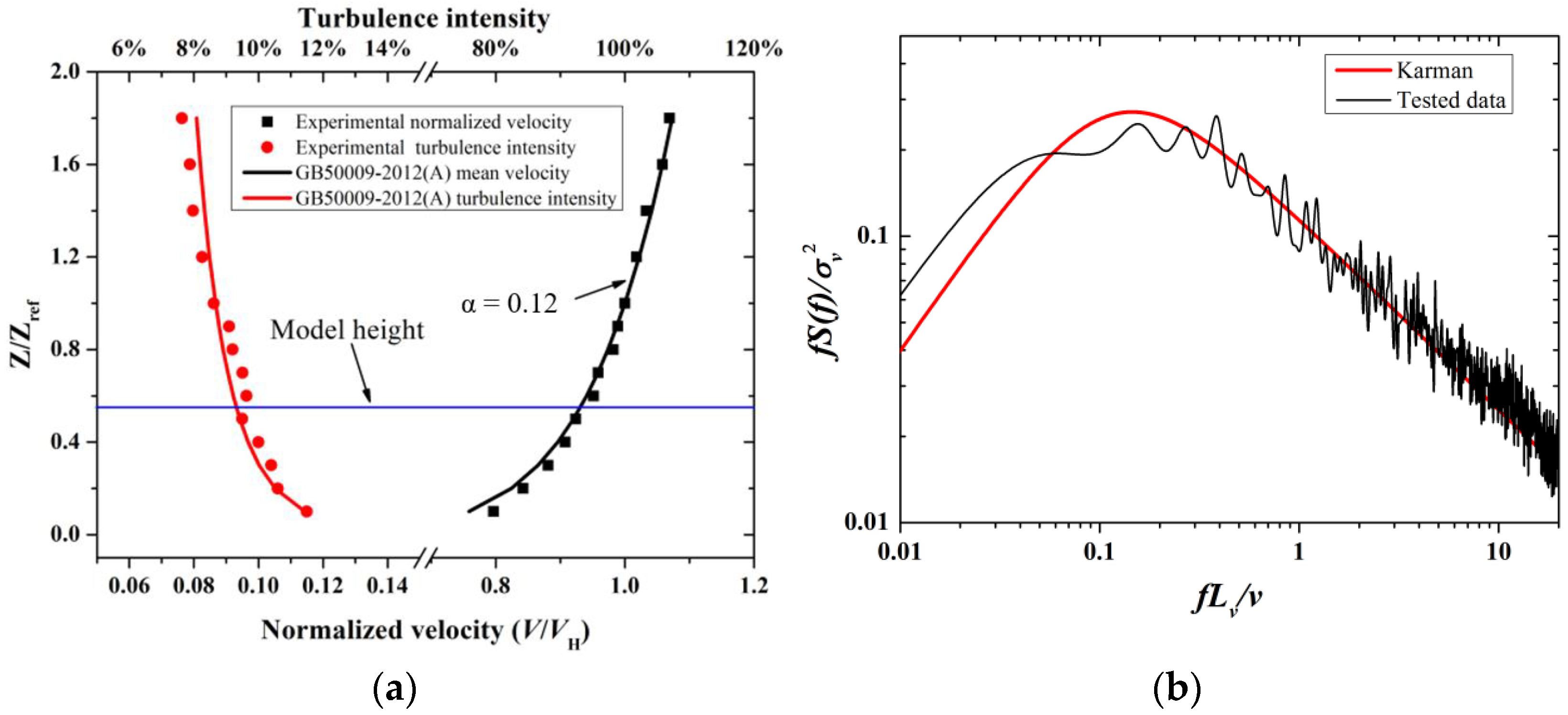
The wind tunnel tests were conducted in the boundary layer wind tunnel at Tianjin Research Institute for Water Transport Engineering (TIWTE). It is a straight-flow wind tunnel with a rectangular test section and an open area in the inlet and outlet of the tunnel. The dimensions of the wind tunnel are 4.4 m × 2.5 m × 15 m (width × height × length). 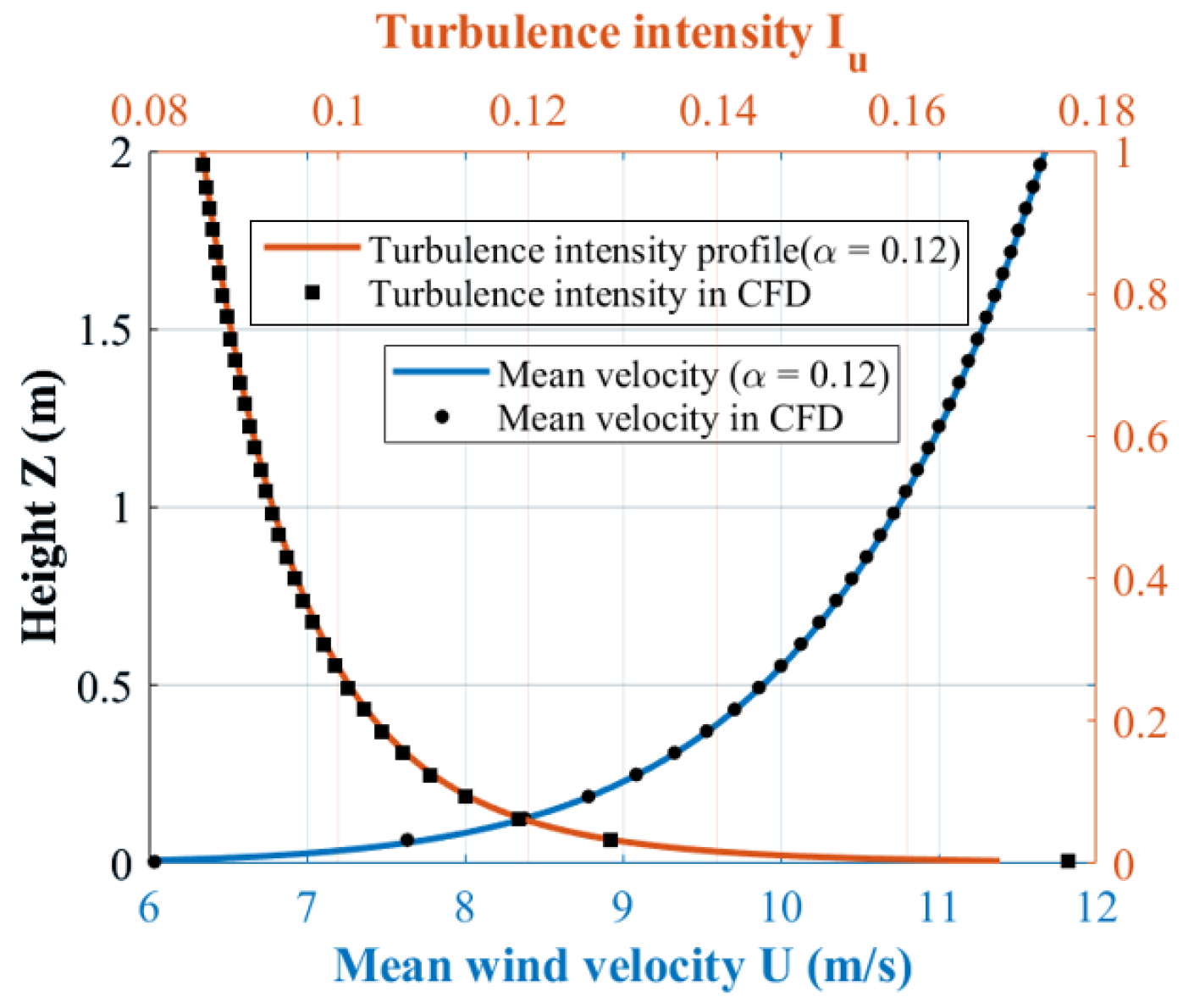In the tests, a coastal atmospheric boundary layer condition (terrain type A in Chinese code [11]) is simulated. The simulated mean wind speed profile was set to follow the power-law profile with an exponent of α = 0.12. The measured mean wind velocity, turbulence intensity profiles, and power spectrum density of fluctuating winds are shown in Figure 4, which are thought to have a good agreement with the code. The boom-down model height, H = 550 mm, was set as the reference height.

Regardless of the Reynolds number when the wind speed is beyond 5 × 10⁵, the mean aerodynamic-force coefficients acting on the crane model have nearly constant values [16]. Within this range of Reynolds number, the wind velocity is set as 10 m/s with a scale of 1:3. The wind velocity is measured in the center of the test location using a TFI Cobra Probe with a sampling rate of 1250 Hz. The reduced power spectrum of the measured wind velocity at the reference height followed the von Karman-type spectrum with an integral length scale of H at the reference height.

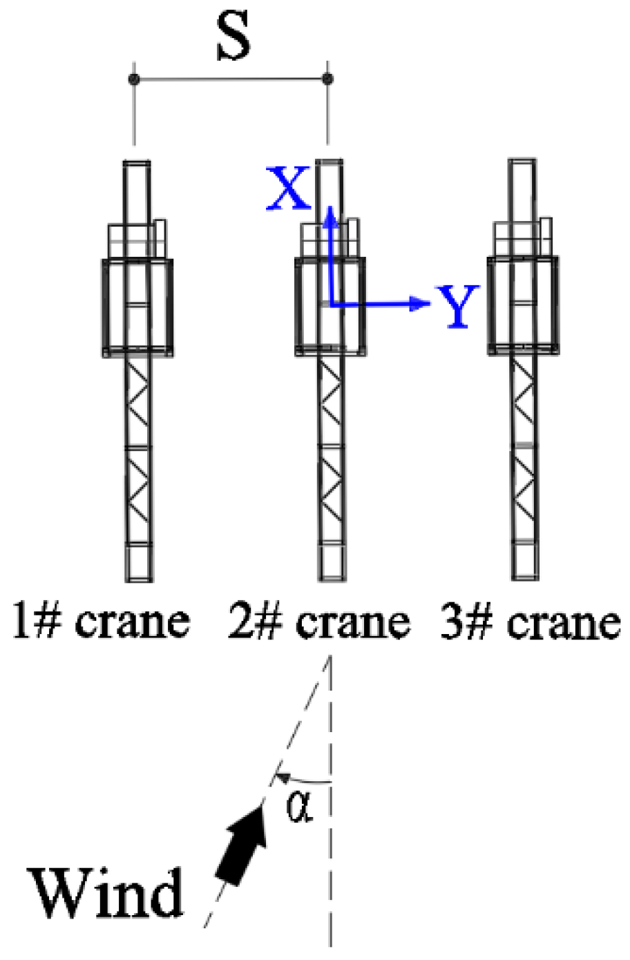
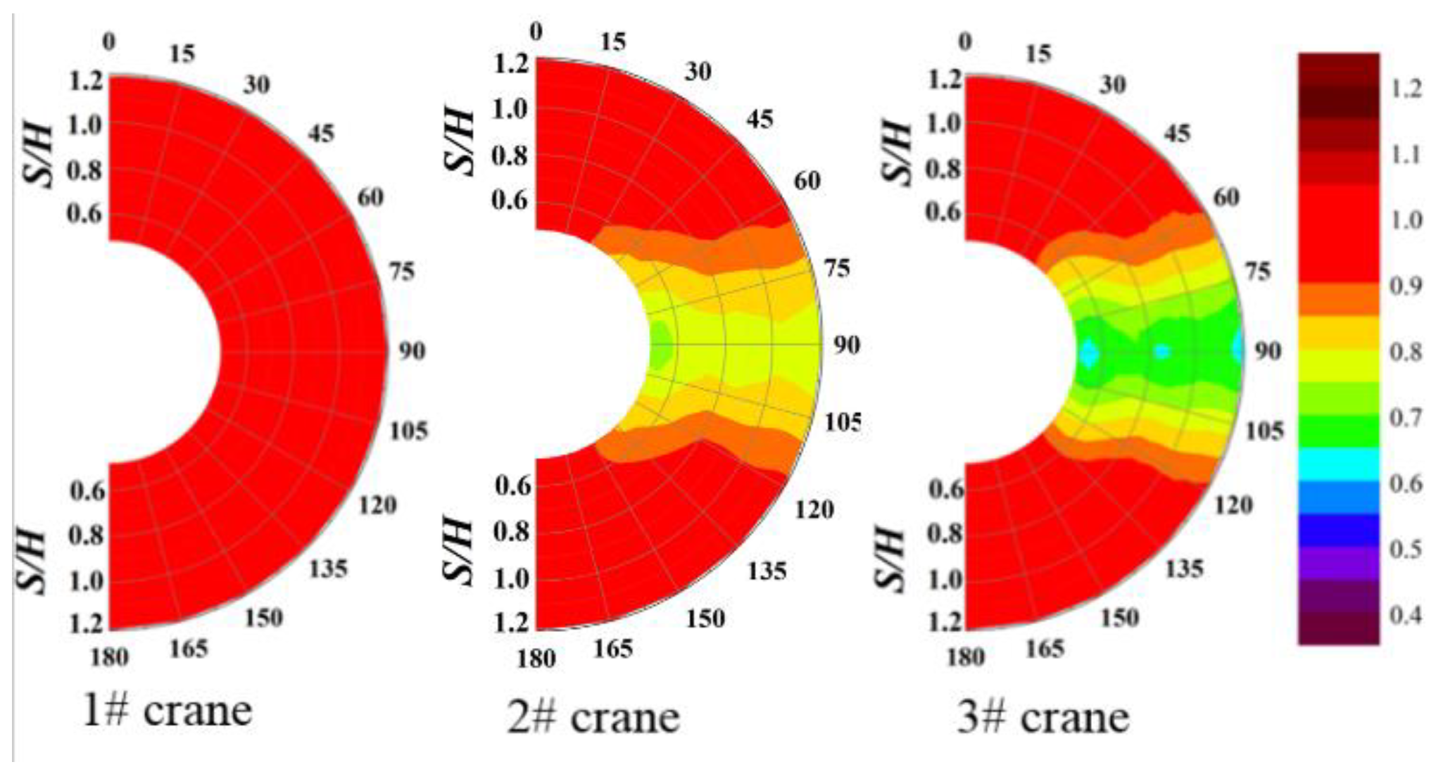
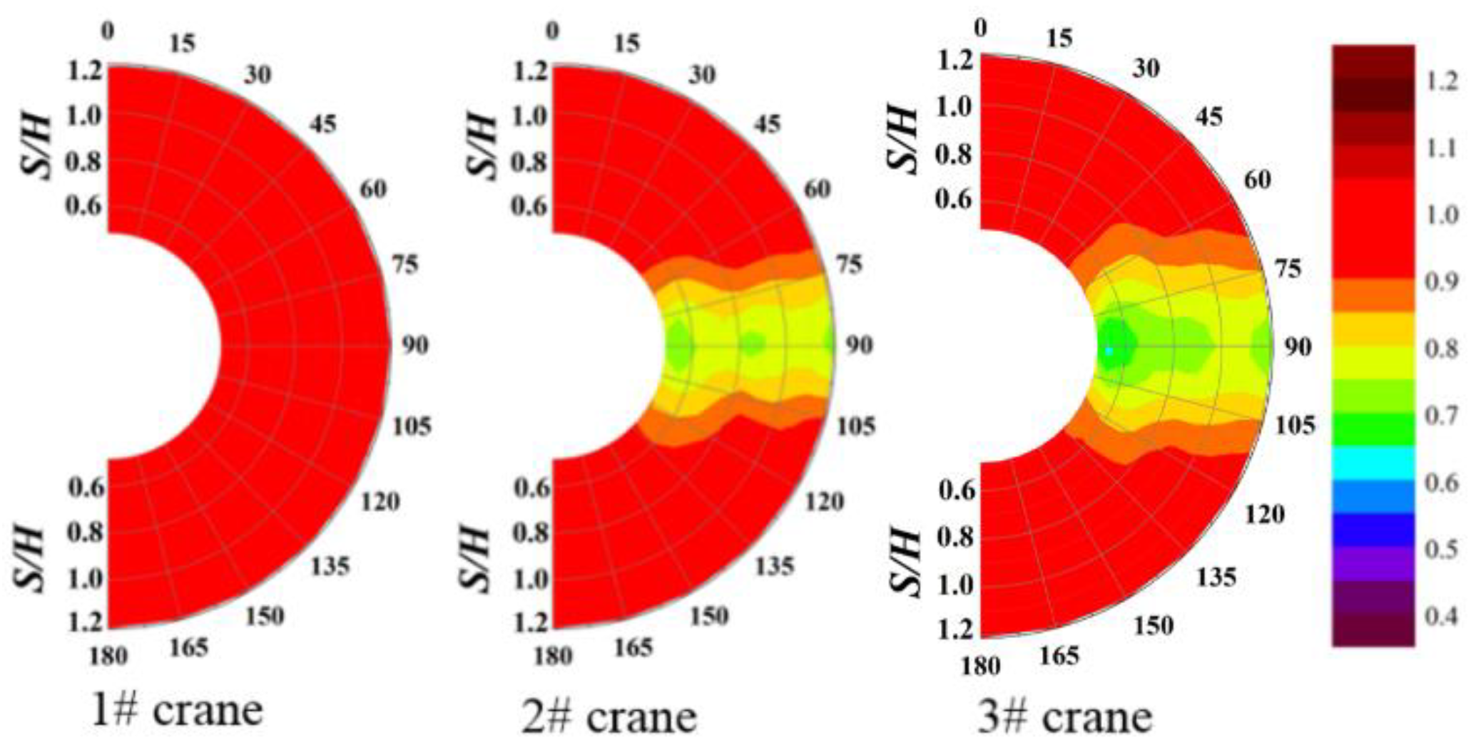
To investigate the interference among the cranes, the three models with the same state were laid in a line for both states. The nondimensional spacing S/H is defined with center spacing S and reference height H. It is set as 0.484, 0.848, and 1.211, which corresponds to 40, 70, and 100 m of the center spacing in the terminals. The top view of the group-arranged crane is demonstrated in Figure 5. The crane models are numbered 1#, 2#, and 3# along the wind direction. When suffering storms, the crane may slide along the rail according to the berthage of the ship, so that the forces along or perpendicular to the rail are always the key design parameter. Thus, the force and moment are decomposed along the body-fitted axis instead of the wind direction axis.

The test model was connected to an ATI Delta high-frequency force balance (HFFB) installed on the center of the turn table. Azimuths of 0°~180° with a step of 15° were tested. A TFI Cobra Probe was installed in the upstream direction at the reference height to measure the reference velocity U_H. As reported in previous studies (Kang & Lee [16], Lee & Kang [17]), the effect of the Reynolds number is negligible in such structures. The test wind speed was approximately 10 m/s at the reference height. The sampling rate (f_s) of the wind force/moment was 1000 Hz, and the duration of sampling (T_s) was 60 s. The test cases are listed in Table 1.

F_i and M_i indicate the forces and moments measured along the body axes, where i is X or Y axis. These wind force/moments were transformed into nondimensional coefficients using the following equations at each sampling time:

$$C_{F_i}=\frac{F_i}{0.5\rho U_0^{2}A}$$

(1)

$$C_{M_i}=\frac{M_i}{0.5\rho U_0^{2}AH}$$

(2)

where A refers to the windward projected area and H is the reference area and reference height, respectively. The mean and root mean square (RMS) values of wind force/moment coefficients ${\overline{C}}_{\lambda }$ and ${\tilde{C}}_{\lambda }$ are calculated by the following equations:

$${\overline{C}}_{\lambda }=\frac{1}{N}{\displaystyle \sum _{i=0}^{N-1}{C}_{\lambda }(t_i)}$$

(3)

$${\tilde{C}}_{\lambda }=\sqrt{\frac{1}{N-1}{\displaystyle \sum _{i=0}^{N-1}{[C_{\lambda }(t_i)-{\overline{C}}_{\lambda }]}^2}}$$

(4)

where $\lambda =F_x,F_y,M_x \mathrm{or} M_y$. It is the arbitrary wind force/ moment component. N is the length of the sampling time points. $t_i$ is the i-th time point of the series. It is proved that the probability distributions of the resultant force coefficient for both isolated and group-arranged cranes obey the Gaussian distribution. And the peak force/moment coefficients ${\hat{C}}_{\lambda }$ are calculated by:

$${\hat{C}}_{\lambda }={\overline{C}}_{\lambda }+g\times {\tilde{C}}_{\lambda }$$

(5)

where g is the peak factor. According to the Davenport Method [34] for calculating the peak factor of a Gaussian process, the value of which is taken as 3.

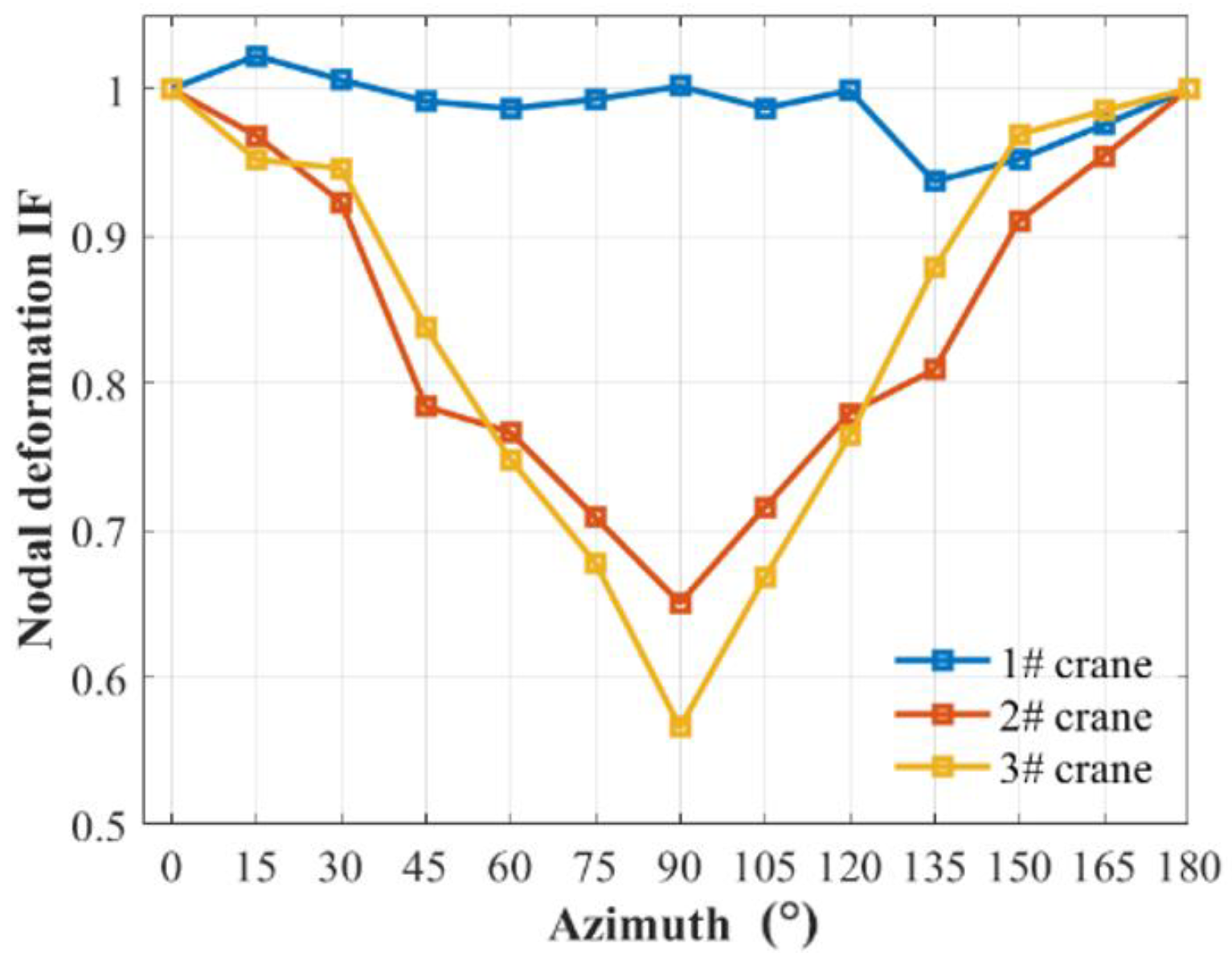
It was found that the RMS wind force/moment coefficients are usually 12~15% of the mean wind coefficients. The most unfavorable cases and the corresponding coefficient values are summarized in

Table 2. The most unfavorable azimuths and values for each wind force/moment coefficient.

Items	Boom Down				Boom Up
	Azimuth	Mean	RMS	Peak	Azimuth	Mean	RMS	Peak
CFx	15/165°	0.80	0.13	1.15	30/150°	0.94	0.19	1.30
CFy	75/105°	1.24	0.16	1.65	60/120°	1.40	0.25	1.82
CMx	75/105°	0.76	0.10	1.05	60/120°	1.08	0.10	1.45
CMy	15/165°	0.47	0.08	0.62	30/150°	0.63	0.06	0.88

. It shows that the most unfavorable cases of C_Fy and C_Mx always occur at 90 ± 15°, and the most unfavorable also occur at the azimuths, which deviate 15° perpendicular to the rail direction.

3.2. CFD Simulation

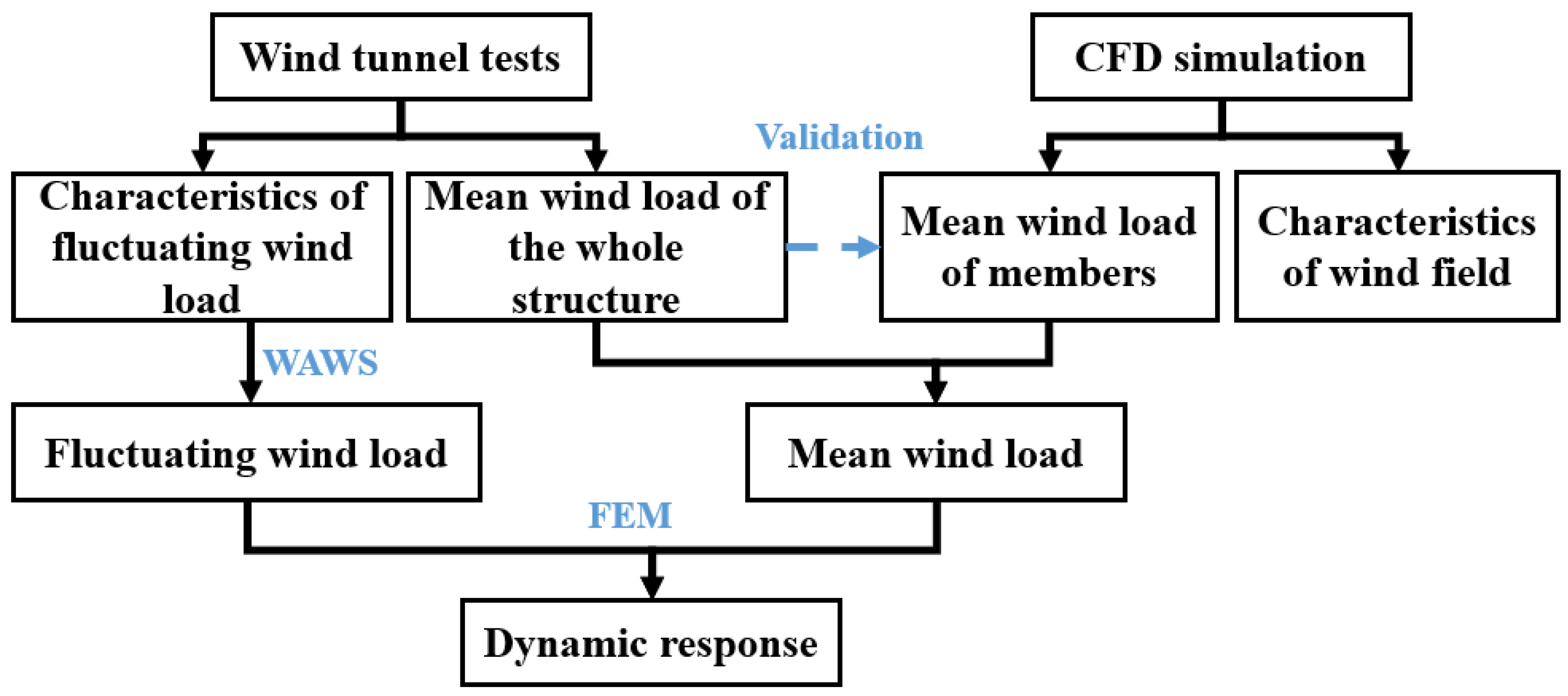
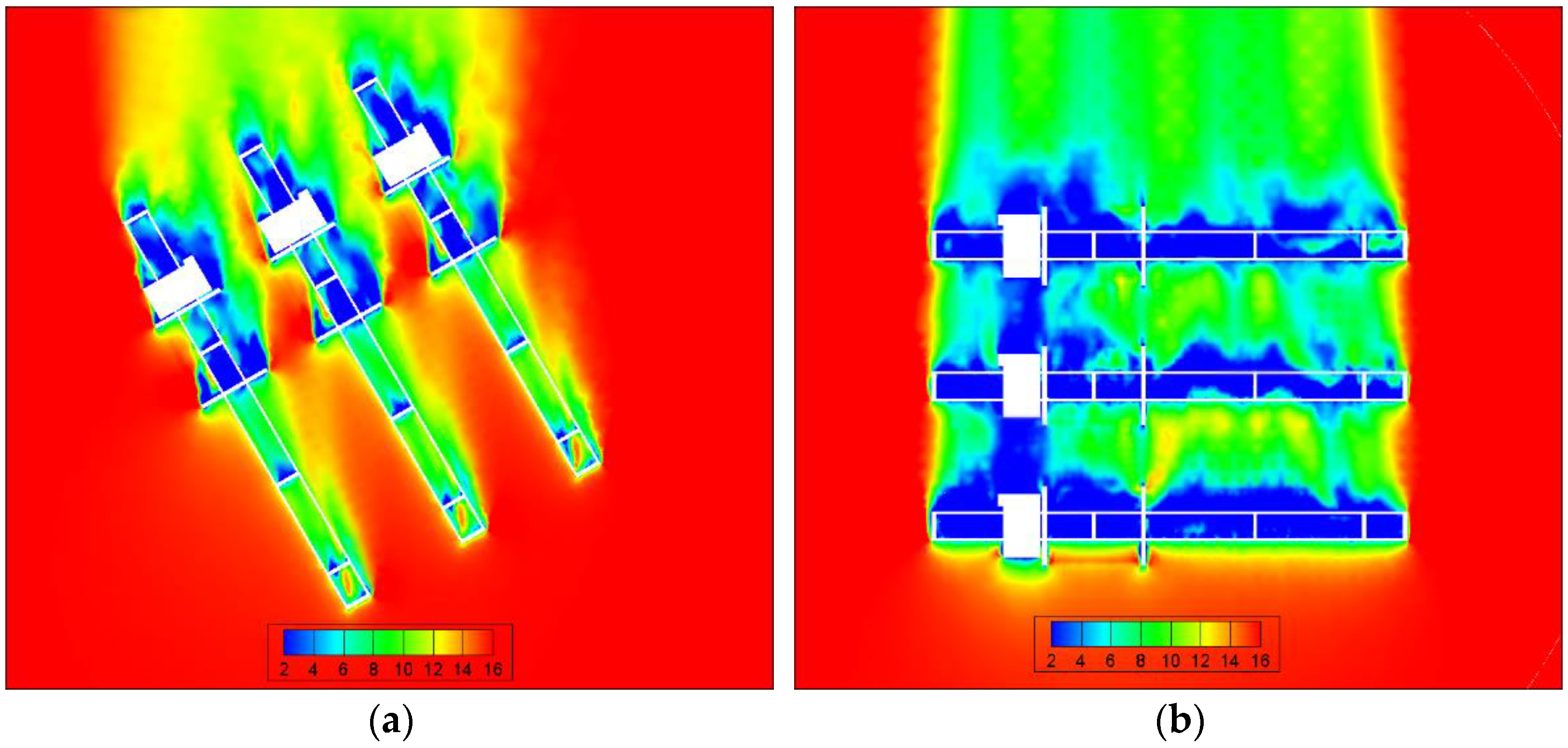
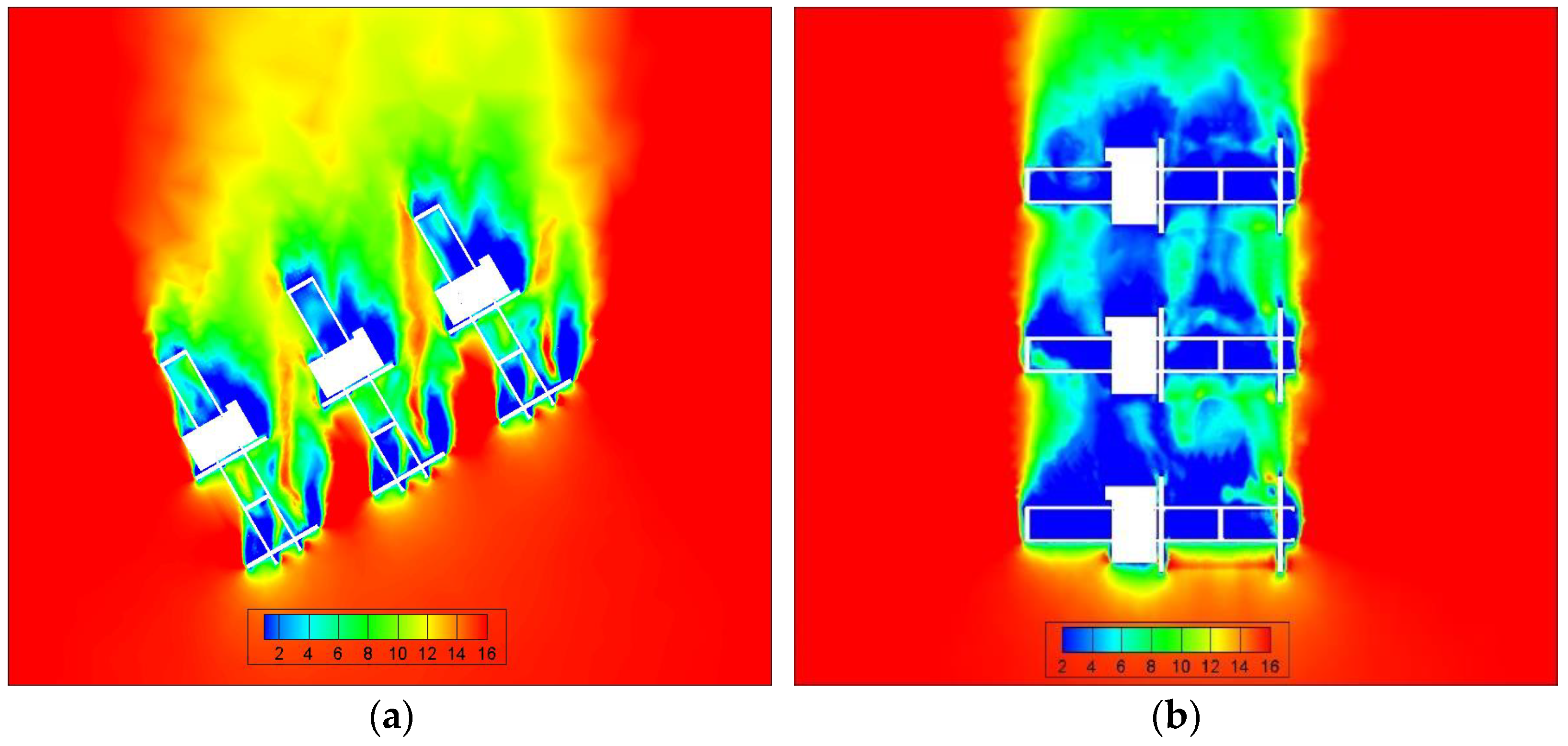
The CFD simulation was carried out to capture the characteristics of the wind field along the structure, aiming to find the root cause of the IE effect on wind loads. Meanwhile, the wind force of each member of each case was obtained, serving as an important supplement for the investigation of wind loads and the preparation of dynamic response calculation.

The CFD simulation was conducted using the Fluent 17.0 software platform. The 3D steady Reynolds stress model (RSM) was adopted in the computation, as it was shown to be appropriate by Huang [15]. The coupling of pressure and velocity was computed using the SIMPLE method. The first-order dispersion scheme was applied for the moment equation, turbulent kinetic energy, and turbulent dissipation rate. According to the convergence standard, all the variables must remain below 10⁻⁴. The same scale and test cases were adopted as those in the wind tunnel tests.

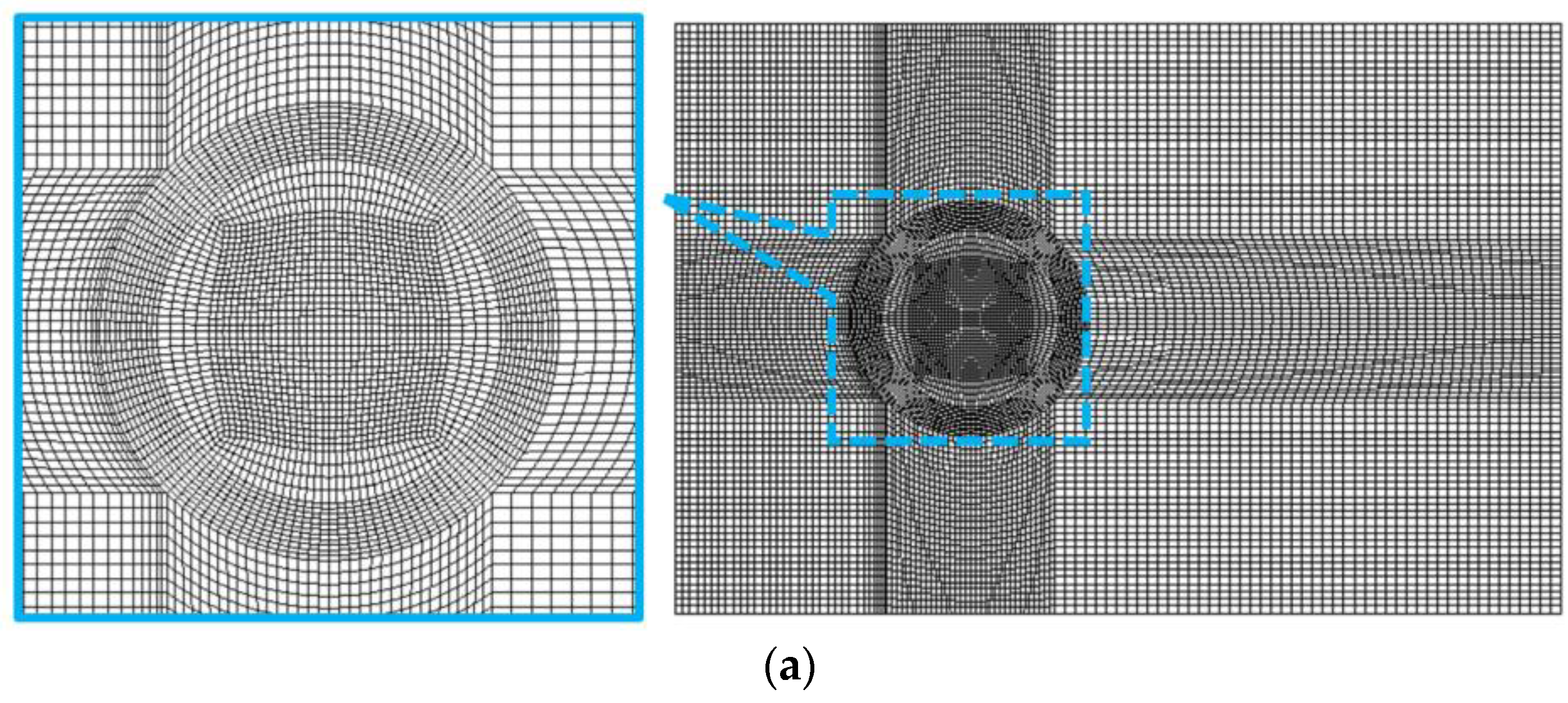
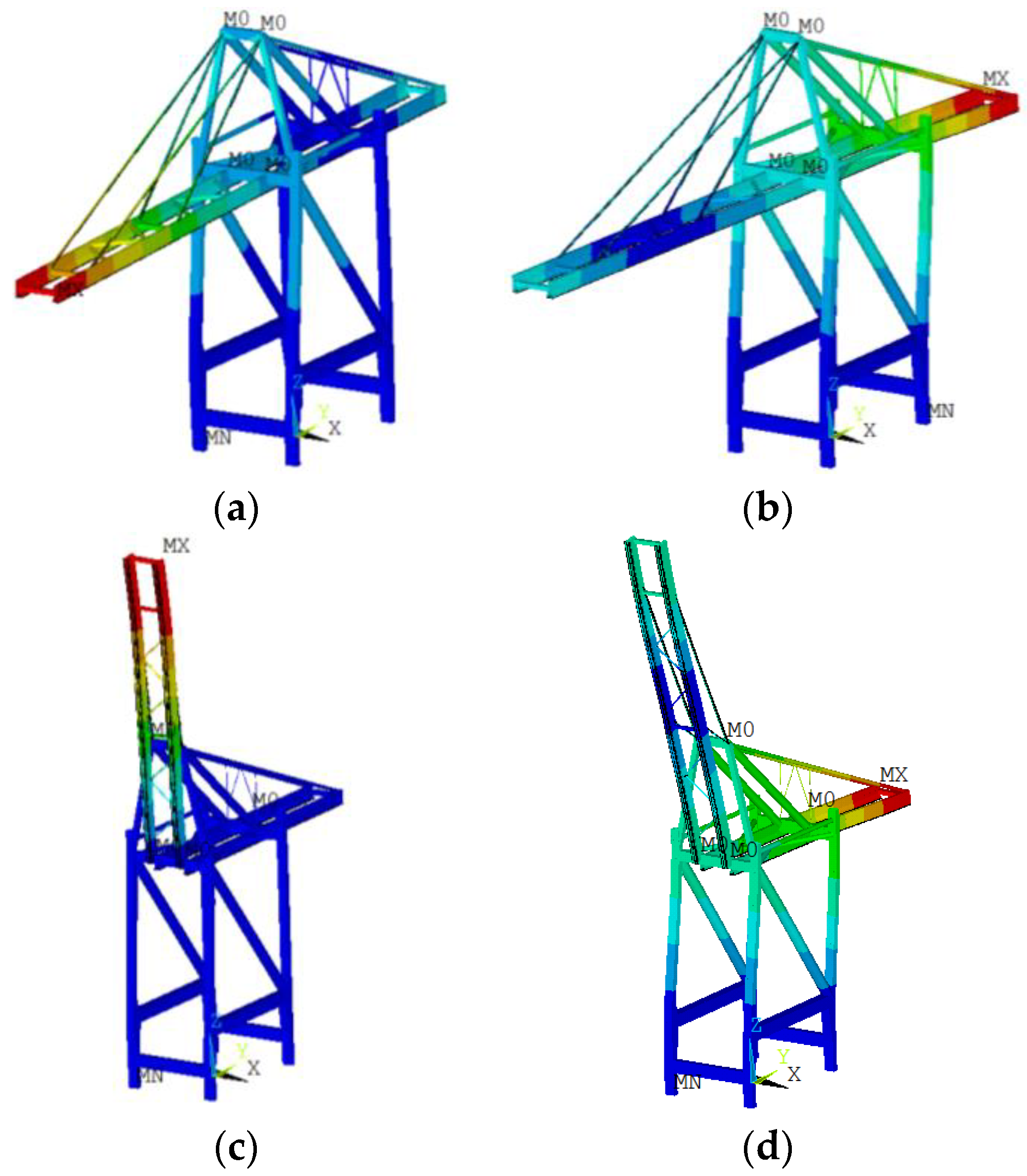
As shown in

Table 3. Parts of the CFD model.

No.	Component Name	No.	Component Name
1	Machine house	9	Inner forestays
2	Boom	10	Brace beams
3	Girder	11	Horizontal beams
4	Portals	12	Legs
5	Sill beams	13	A-frame beams
6	Backstays	14	Restrictions
7	Upper diagonals	15	A-frame
8	Outer forestays

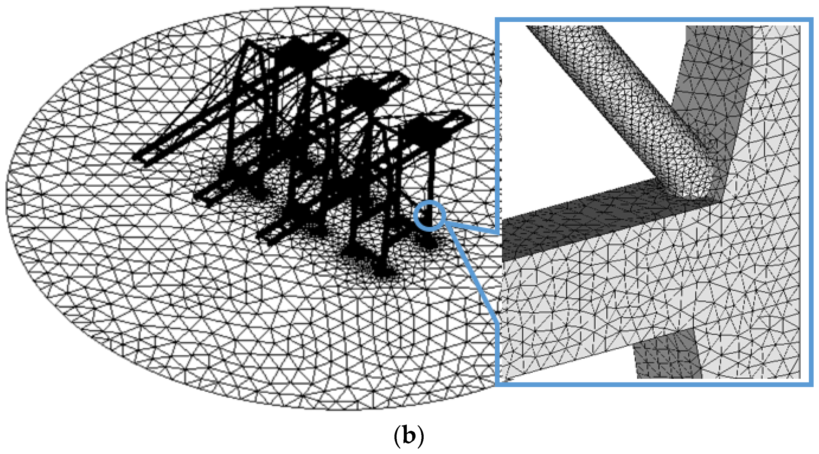
, the CFD model is divided into 15 parts according to the category of the members in the code. Because of the complicated geometry of the model, the computational domain is divided into a cylindrical interior field and an exterior field. Unstructured tetrahedral meshes are applied in the interior area, and structured hexahedral meshes are used in the outer area (Figure 6). The interior mesh is denser to better capture the airflow characteristics around the model. The grids are merged in nodes on the surface between two fields, so the boundary condition of the surface is set as ‘Interior’. The area around the main and diagonal members is encrypted by constructing a 10-layer boundary layer grid with an equal growth ratio of 1.1. The total number of meshes reaches 7 million. The mesh outside the interior domain is constant. So only the interior part is changed according to the model (isolated or group-arranged ones), spacing, and azimuth. The dimensions and the boundary condition of the computation domain are demonstrated in Figure 7. The computational domain is configurated as a simple rectangular box. It has dimensions of 3.33 × 6.67 × 10 m³ (500 × 1000 × 1500 m³ for prototype model) to ensure the magnitude is larger than 5, 40, and 15 times of the height, width, and length of the crane model. The maximum the blockage ratio is less than 1%.

The mesh independency analysis is performed in this study. The trial test of the C_Fy is performed by varying the number of meshes, and the results obtained are shown in

Table 4. C_Fy values for different numbers of meshes.

Number of meshes (million)	3.54	5.38	7.58	11.46
CFy	1.234	1.206	1.195	1.191
Error (%)	3.87	1.47	0.58	0.22

. Despite the number of meshes varying widely, the calculated C_Fy are similar, with an error of 3.2%, and 5.38 million meshes satisfied the calculation requirements and could guarantee high calculation efficiency. After comprehensive consideration, the 7.58 million mesh scheme was conservatively used in the subsequent analysis.

For mean wind velocity U (in m/s), the target vertical profile is the same as the wind tunnel one. The velocity inlet is set according to the following equations:

$$U(z)=U_{ref}{(\frac{z}{z_{ref}})}^{\alpha }$$

(6)

with z_ref = 550 mm (equal to H), U_ref = 10 m/s and α = 0.12. As shown in Figure 8, the CFD inlet profiles for mean wind velocity and turbulence intensity agree well with that specified in the codes. The vertical profile of turbulent kinetic energy k over height z is calculated based on the target mean velocity profile and the turbulence intensity above the ground.

$$k(z)=I_U{(z)}^2\cdot U{(z)}^2$$

(7)

The turbulence dissipation rate ε (m²/s³) is calculated as

$$\epsilon (z)=\frac{u^{*3}}{\kappa (z+z_0)}$$

(8)

where κ is the von Karman constant (κ = 0.4) and u* the friction velocity calculated by

$$u^{*}=\frac{\kappa \cdot U_{ref}}{\ln (\frac{z_{ref}+z_0}{z_0})}$$

(9)

The aerodynamic roughness length for the ground plane of the domain representing water was derived from the updated Davenport roughness classification z₀ = 0.0002 m [35]. The test cases of the CFD simulations can cover those of wind tunnel tests. Furthermore, the spacing of the model in the CFD cases is smaller for both two crane states, which is set as 40~100 m with a step of 10 m.

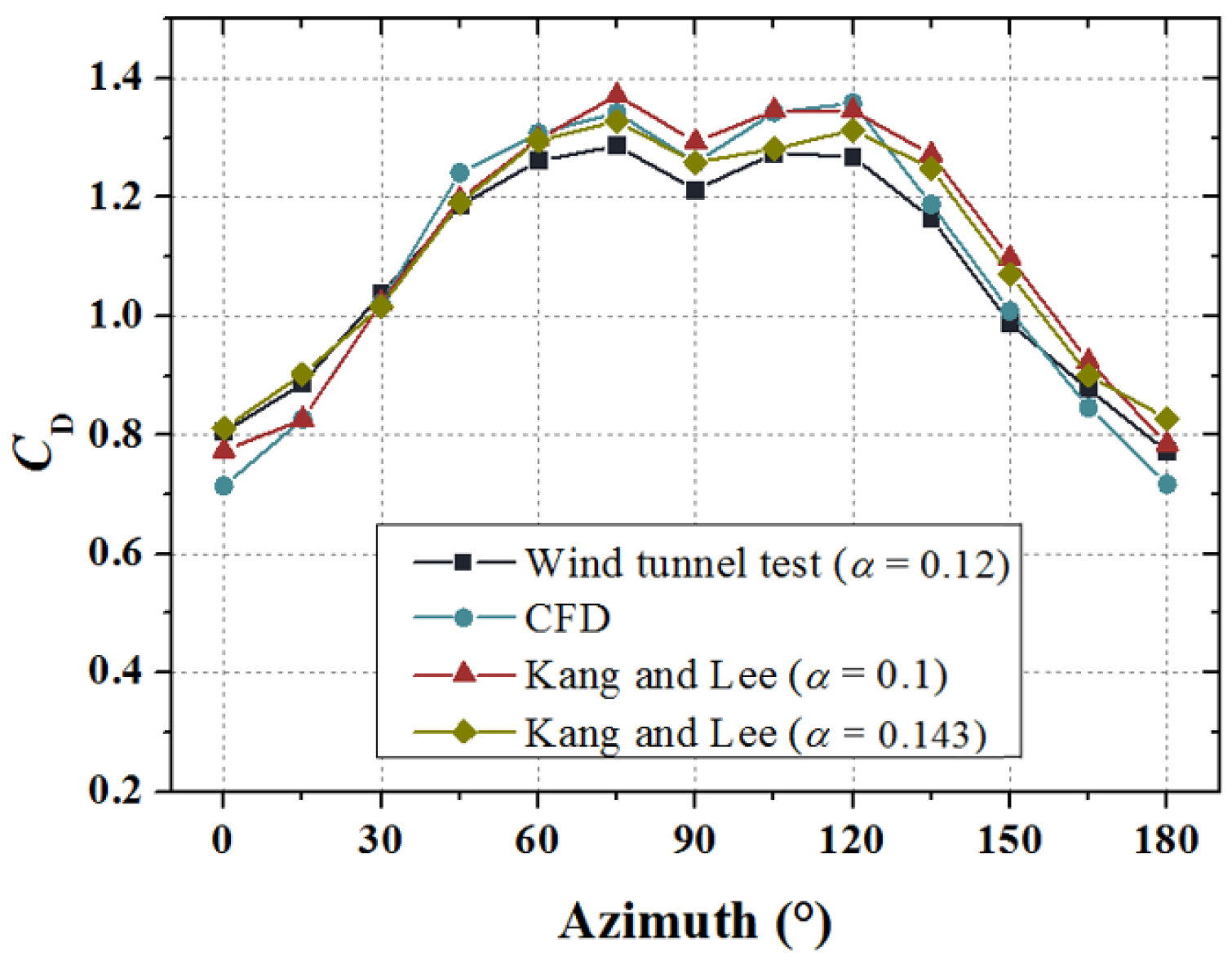
The mean drag coefficient values for the boom-down crane in the wind tunnel test are shown in Figure 9. For comparison, the results of Kang and Lee’s [16] wind tunnel test with the pow-law exponents of 0.143 and 0.1 are also demonstrated in the figure. The results obtained in the current study are in good agreement with previous investigations. The most unfavorable azimuth is 75° for the boom-down state in the wind tunnel tests, which also corresponds with the conclusions drawn by Kang and Lee [16]. Additionally, the wind force of each member was obtained and validated by wind tunnel tests, and the results were applied when calculating the wind-induced response. Moreover, the force and moment coefficients of CFD simulation in all cases were compared with that of the wind tunnel tests to check the accuracy. 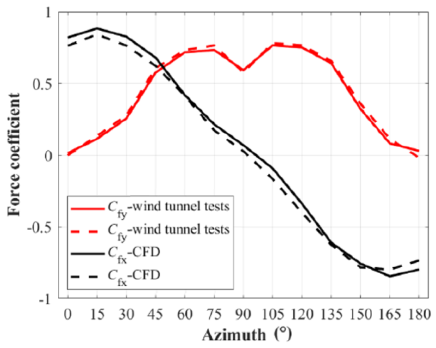As shown in Figure 10, the force coefficient of 3# crane in case 3 was demonstrated and showed that the results agreed well.

3.3. Stochastic Simulation

Based on the wind tunnel tests, the wind force of the individual members was assumed to have the same wind load characteristic as that of the whole body (Xiao et al. [18]). In addition, the same mean root square of wind force was used. Katagiri [36] noted that the nondimensional auto-power spectrum of the wind load is independent of the height. Thus, $S_F(f)$ can be expressed as follows:

$$S^{\prime }{}_F(f)=\frac{S_F(f,z_i)}{{\sigma }_F^2(z_i)}=\frac{S_F(f,z_j)}{{\sigma }_F^2(z_j)}$$

(10)

where $S^{\prime }{}_F(f)$ is the nondimensional auto-spectrum, ${\sigma }_F$ is the RSM of the wind force of each member (assumed to be the same as that for the whole structure), and $z_i$ is the height of the i-th member (determined according to [37]). The cross-power spectrum $S_{Fij}(f,z_i,z_j)$ can be simplified as

$$S_{Fij}(f,z_i,z_j)={\sigma }_F(z_i){\sigma }_F(z_j)S^{\prime }{}_F(f)coh(p_i,p_j)$$

(11)

where $coh(p_i,p_j)$ [37] is the coherence function of the wind load between members. $p_i$ and $p_j$ is the coordinate of the i-th and j-th member. It is related to the position of the member. Therefore, the spectrum of the base moment can be deduced as

$$S_M(f)={\displaystyle \sum _{i=1}^N{\displaystyle \sum _{j=1}^N{S}_{Fij}(f,z_i,z_j)}}{z}_i{z}_j$$

(12)

according to Equation (11), it can be expressed as,

$$S_M(f)={\displaystyle \sum _{i=1}^N{\displaystyle \sum _{j=1}^N{\sigma }_F(z_i){\sigma }_F(z_j)S^{\prime }{}_F(f)coh(p_i,p_j)}}{z}_i{z}_j$$

(13)

Thus,

$$S^{\prime }{}_F(f)=\frac{S_M(f)}{{\displaystyle \sum _{i=1}^N{\displaystyle \sum _{j=1}^N{\sigma }_F(z_i){\sigma }_F(z_j)coh(p_i,p_j)}}{z}_i{z}_j}$$

(14)

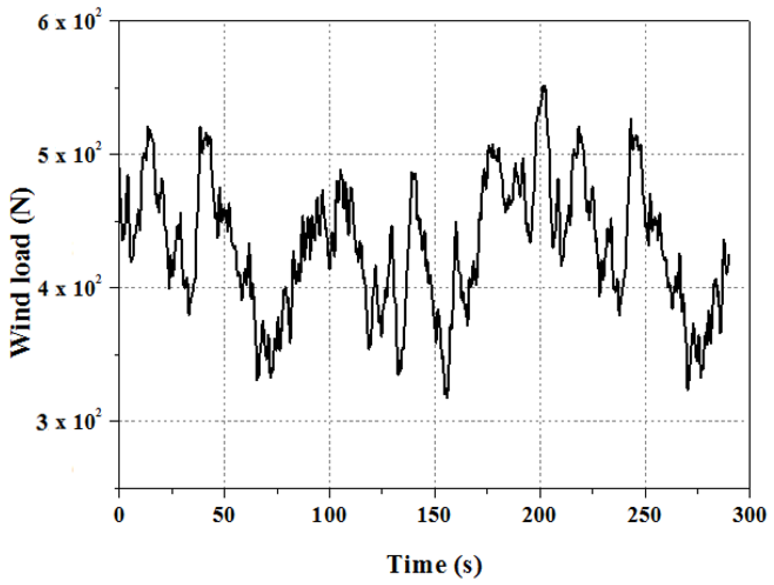
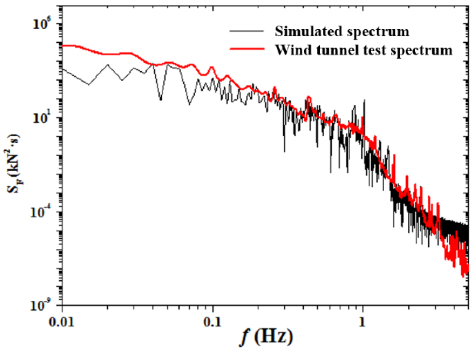
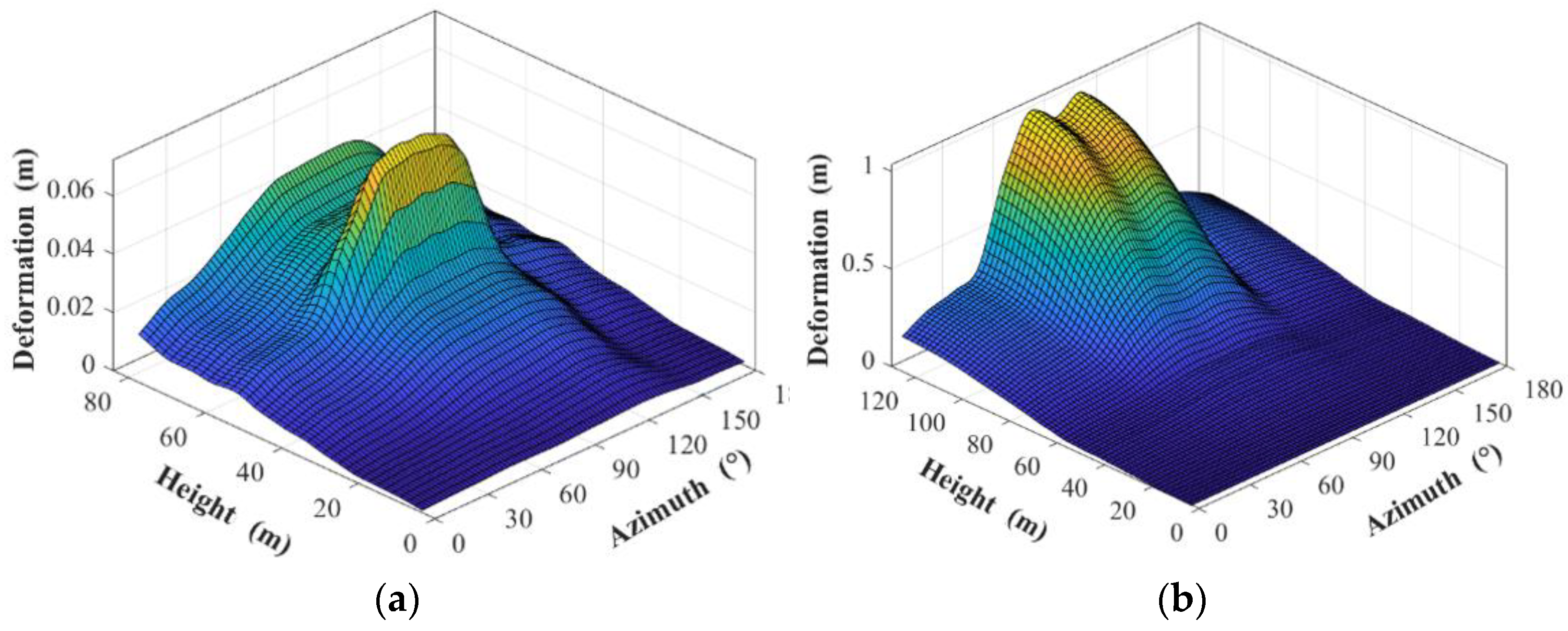
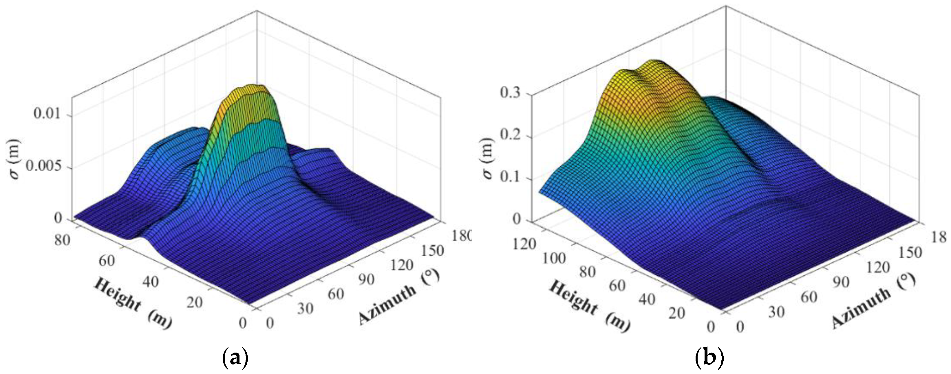
where the spectrum of the base moment $S_M(f)$ can be deduced by the results of the HFFB tests. According to Equation (14), the wind force history of members can be generated according to the moment spectrum and the fluctuating wind force coefficients obtained in the wind tunnel tests. Based on the above deduction, the WAWS was carried out and wind load time history of each member was obtained. Each element in the FEM model, corresponding to each member, was meshed uniformly with several nodes. The wind load of the member was distributed uniformly on nodes attached on it. The wind load time history on the top point of the boom-down crane generated by WAWS is shown in Figure 11. As shown in Figure 12, the sum of the members’ wind force time history is calculated as the base shear force, which was compared with the results of the wind tunnel tests of the corresponding case.

4. Discussion

4.1. Interference Effects of Wind Loads

To investigate the interference effect, container cranes were arranged in a line, similar to their arrangement in ports and terminals. To study the interference effect more quantitatively, we introduced the interference factor [38] (IF, also known as buffeting or shielding factor) to assess the interference effects imposed by the surrounding structures quantitatively:

$$IF=\frac{F_{\mathrm{g}}}{F_i}$$

(15)

where F_g and F_i represent the force on a group-arranged building considering the IE and force on an isolated building, respectively. IF < 1 means that the IE will reduce the wind load of the crane. IF > 1 means that the IE will increase the wind load. We calculated the mean interference factor (MIF), dynamic interference factor (DIF), and extreme interference factor (EIF) by force or moment coefficients ${\overline{C}}_{\lambda }$, ${\tilde{C}}_{\lambda }$, and ${\hat{C}}_{\lambda }$ defined previously.

The MIF of the group-arranged cranes with S/H = 0.484~1.211 for both states are demonstrated in Figure 13 and Figure 14. It was found that the minimum IF is 0.6 and 0.7 when α = 90° with minimum spacing for boom-down and boom-up states, respectively. A more significant and larger influence range was found in boom-down cranes compared with the corresponding cases of boom-up cranes, noting the factor is always smaller in the boom-down state. The IE is more dominant on crane 3# as compared to crane 2# because of the presence of one more upstream structure. The factor reduces by 13% and 18% as a windward shielding crane locates when α = 90° with minimum spacing. This influence becomes less dominant as wind direction deviates 90°. In addition, as the spacing changes larger, the influence range of the interference effect became smaller and less dominant. As for crane 2#, an interference effect can be observed in α = 30°~150° when S/H = 0.484, while the range shrinks to about 60~120° for the boom-down crane. A similar tendency can also be determined in crane 3# and boom-up state. However, crane 1#, the upstream one, is not affected by the interference effect regardless of the nondimensional spacing and crane state. The IF of these cases is always around 1.0.

Table 5. Maximum MIF with different spacings.

Nondimensional Spacing	Interference Factor
	MIFMx						MIFFy
	Boom-Down			Boom-Up			Boom-Down			Boom-Up
	Value	Position	α	Value	Position	α	Value	Position	α	Value	Position	α
		No.	(°)		No.	(°)		No.	(°)		No.	(°)
0.484	2#	15	1.000	2#	15	1.020	1#	15	1.002	1#	15	0.981
0.848	2#	15	1.000	2#	30	1.031	1#	15	1.006	2#	30	1.022
1.211	2#	15	1.018	2#	60	1.041	1#	15	1.032	1#	60	1.002

,

Table 6. Maximum DIF with different spacings.

Nondimensional Spacing	Interference Factor
	DIFMx						DIFFy
	Boom-Down			Boom-Up			Boom-Down			Boom-Up
	Value	Position	α	Value	Position	α	Value	Position	α	Value	Position	α
		No.	(°)		No.	(°)		No.	(°)		No.	(°)
0.484	1.165	3#	165	0.983	1#	60	1.243	3#	165	0.987	1#	60
0.848	1.126	3#	165	1.009	3#	45	1.217	3#	165	1.014	3#	45
1.211	1.088	3#	165	1.052	1#	60	1.140	3#	165	1.046	1#	60

and

Table 7. Maximum EIF with different spacings.

Nondimensional Spacing	Interference Factor
	EIFMx						EIFFy
	Boom-Down			Boom-Up			Boom-Down			Boom-Up
	Value	Position	α	Value	Position	α	Value	Position	α	Value	Position	α
		No.	(°)		No.	(°)		No.	(°)		No.	(°)
0.484	1.060	3#	165	0.988	1#	15	1.116	3#	165	0.984	1#	60
0.848	1.054	2#	15	0.982	1#	30	1.104	3#	165	0.994	1#	30
1.211	1.022	3#	180	1.028	1#	60	1.064	1#	180	1.036	1#	60

provide the maximum values of MIF, DIF, and EIF as well as the occurrence cases under different nondimensional spacings. The following findings can be observed:

• For the mean wind load, the maximum interference factor occurred in boom-down crane 1# for S/H = 0.484. The amplification of the mean wind load is not dominant in the case of group-arranged cranes, indicating that the influence of the interference effect on the mean wind load can be neglected;
• For the dynamic wind load, the DIF of the boom-down cranes is always high, which is similar to the distribution of EIF values. In addition, the maximum DIF always occurred when α = 165°. Amplification of the wind loads is observed in some cases of boom-down cranes, especially for crane 3#, and the effect became more dominant as the spacing became smaller. However, the IE is negligible among boom-up cranes;
• The interference effect is more obvious in the DIF and MIF. Values of the three IF exhibited different distributions. The value of the DIF is higher and the maximum is 1.24, indicating fluctuating wind loads may increase more than 20% for the boom-down crane 3#;
• Though the RMS and peak wind forces are amplified in some cases, the most unfavorable case in terms of the peak wind force coefficients do not change significantly. It attributes that the most unfavorable cases are always the cases in which IE reduces the wind loads.

To explain the phenomenon and mechanism of IE on the group-arranged cranes, two cases of α = 30° and 90° with minimum spacing are shown in this section. The contour plots of the horizontal wind velocity for both states of group-arranged cranes are shown in Figure 15 and Figure 16 respectively. The boom height (57 m in prototype) is selected for the slice plane. And the wave flow around the jib and machine house can be demonstrated. It is found that when α is or near 90°, more members are hidden behind from the windward structures, 1# or 2# crane. As shown in Figure 15a, compared with that of the boom-up state, when the jib is horizontally settled in the boom-down state, more windward members are shielded. Though the wake flow may enhance turbulence, the shading effect is always dominant and tends to reduce wind loads. Thus, the IE is thought as the combined effects of both the shielding effect and the amplification of turbulence. As for the boom-down crane at α = 165°, the shielding effect is so wake that the turbulence generated by the wave flow amplified the extreme wind loads. However, because of the lifting boom, the windward boom-up crane mainly affects the seaside girder and part of the machine house. Thus, IE is less obvious than that of the boom-down crane and the factor is near 1.

4.2. Interference Effects of Wind-Induced Response

The prototype finite element model was established using the ANSYS 17.0 software platform. Yield stress for the two main types of steel, Q345, and Q235, were 310 and 215 MPa, respectively. Q235 is mainly used in auxiliary materials, whereas Q345 is widely used in the main material. Beam 188 and Mass 21 elements were, respectively, used to simulate the members and the mass of the auxiliary facilities, such as machine houses and lifts. By using the subspace method in the modal analysis, the first three natural frequencies and the vibration modal characteristics were obtained, as shown in

Table 8. The first five natural frequencies of the quayside container crane models.

No.	Frequency/Hz
	Boom Down	Boom Up
1	0.335	0.289
2	0.527	0.527
3	0.727	0.800
4	1.091	0.867
5	1.434	1.214

. The first two modal shapes are shown in Figure 17.

The design wind velocity [12] for both boom-down and boom-up quayside container crane is 20 m/s and 40 m/s (3 s gust wind speed) for the quayside crane. The same value was specified in our research for both isolated and group-arranged cranes. The transient dynamic full-time history analysis can then be conducted using the Newmark-β method. The damping ratio is set as 2% and the collection period is 660 s (the first 60 s is discarded avoiding the impact effect). Both wind load and self-weight were considered. According to the nodal deformation wind vibration coefficient ${\beta }_i$ is adopted, which can be calculated by the following two formulas:

$${\beta }_i=\frac{{\overline{r}}_i+r_i}{{\overline{r}}_i}=1+\frac{\mu {\sigma }_i}{\overline{r}}$$

(16)

$${\sigma }_i{}^2={\displaystyle {\sum }_{j=1}^n{(R_j-{\overline{r}}_i)}^2/(n-1)}$$

(17)

where ${\sigma }_i$ is the mean square error of the deformation of i-th node. $\mu$ is gust loading factor and is taken to be 2.5 [39]. ${\overline{r}}_i$ is the mean deformation. $r_i$ is the RMS value of fluctuating deformation. $R_j$ is the j-th sampling point of the time history for the deformation response, which can be obtained by the dynamic analysis of the structure under instantaneous wind loads. n refers to the number of sampling points.

The ū and σ of displacements for both isolated boom-up and boom-down cranes are shown in Figure 18 and Figure 19. The maximum ū and σ displacements always occur at the far end of the crane jib (node 119 for boom-down and node 174 for boom-up state), the height of which is 52 m and 125 m for boom-down and boom-up states, respectively. And these points are also the peak points of the displacement surface locates, which are 0.072 m and 1.01 m for maximum mean deformation and 0.012 m and 0.27 m for maximum RSM deformation. According to the ū and σ deformation surface, 75~105°are the unfavorable azimuths. The maximum wind vibration coefficient is 1.42 and 1.70 for the boom-down and boom-up cranes, respectively.

The response of the nodes with maximum deformation, that is node 119 for the boom-down state and node 174 for the boom-up state, when α = 90° and S/H = 0.484 of both states are demonstrated in Figure 20. In these cases, the IE is the most obvious. As for the freestanding crane, both peak and mean deformation do not change considerably. It attributed to the similar distribution of wind loads for 1# group-arranged crane and isolated one. As for the 3# crane, the peak value of the node deformation is 0.1 m and 1.8 m, with the IF of 0.56 and 0.70 for boom-down and boom-up state respectively. According to the dynamic response, the group arrangement is suggested when suffering storms or typhoons.

Figure 21 and Figure 22 show the IF for peak deformation of boom-down and boom-up 3# crane respectively. The nodes of the jib and upper parts, with a height of more than 57 m, are proven to have a more significantly reduce in peak dynamic deformation when α = 60~120°. Similar to the tendency in wind loads, a larger influence range of IE is found in the boom-down crane compared with that of the boom-up one. Figure 23 and Figure 24 show the IF for peak deformation of the endpoint of the jib for the boom-down and boom-up crane respectively. It was found that the curves have a similar tendency with those of the wind load interference factor, with more members hidden back from the windward ones. The cases with favorable interference effects always occur near α = 90°. Although in some cases the dynamic wind loads were increased by up to 16%, the IE did not increase the dynamic response of most unfavorable cases (isolated cranes) significantly. The maximum IF is 1.054 at the end of the jib for the boom-down 3# crane with α = 165°. The amplification in the dynamic response of the IE is not obvious and it does not occur in the most unfavorable azimuth. Therefore, the current codes could envelop the amplification in the dynamic response of the IE.

5. Conclusions

A series of wind tunnel tests on 1:150 scaled-down isolated and group-arranged quayside cranes models is conducted using the HFFB tests. CFD simulations of the corresponding cases were conducted for verification. Under different wind incidence azimuths, the force and moment coefficients along or vertical to the rail of the whole crane body or isolated members were obtained. Based on the tests and simulation, the wind force time histories were generated by WAWS, and the wind-induced responses were analyzed according to the finite element models. The main findings of the study are summarized as follows:

• Based on the results of HFFB, the wind load spectra were deduced. WAWS was applied to generate fluctuating wind forces. Combined with the mean wind loads obtained by CFD simulation, the wind-force time history of each member was generated. The proposed analysis method was first applied on the quayside container cranes;
• The most unfavorable azimuth of the boom-up and the boom-down crane is 75°/105° and 60°/120°, respectively. In some cases, the fluctuating wind loads can increase by up to 16%, while the wind loads of most unfavorable cases will not change greatly. The minimum IF is 0.6 and 0.7 for boom-down and boom-up crane, respectively;
• The interference effect is thought as the combined effects of both shielding effect, which reduce the wind load, and the amplification of turbulence. The shielding effect always exerts a greater influence on the boom-down cranes with less center spacing and becomes more dominant when the wind direction approaches 90°;
• Similar to the wind load patterns, the IE mainly reduced the wind response. The minimum interference factor of peak nodal deformation is 0.59 and 0.70 for the boom-down and boom-up crane respectively. The group arrangement is suggested when suffering storms or typhoons. Furthermore, the current codes could cover the amplification in the wind-induced response of the IE.

References

1. McCarthy, P.; Soderberg, E.; Dix, A. Wind damage to dockside cranes: Recent failures and recommendations. Lifeline Earthquake Engineering in a Multi-hazard Environment. In Proceedings of the American Society of Civil Engineers Technical Council on Lifeline Earthquake Engineering Conference (TCLEE), Oakland, CA, USA, 28 June–1 July 2009. [Google Scholar]
2. Zhang, C.H.; Sun, W.; Peng, X.Q. Numerical simulation of interference effects on the port container groups under strong wind. J. Huaqiao Univ. Nat. Sci. 2010, 31, 69–73. [Google Scholar]
3. BS 2573-1; British Standard. Rules for the Design of Cranes Part 1: Specifications for Classification, Stress Calculations, and Design Criteria for Structures (4th Revision). BSI: San Jose, CA, USA, 1983.
4. Gur, S.; Chaudhuri, S.R. Vulnerability assessment of container cranes under stochastic wind loading. Struct. Infrastruct. Eng. 2014, 10, 1511–1530. [Google Scholar] [CrossRef]
5. Jordan, M.A. Dockside container cranes: Reprinted from PORTS ’95. In Proceedings of the Sponsored by the Committee on Ports and Harbors of the Waterway, Port, Coastal, and Ocean Engineering Division/ASCE, Tampa, FL, USA, 13–15 March 1995. [Google Scholar]
6. McCarthy, P.; Jordan, M.; Lee, K.; Werner, S. Increasing hurricane winds dockside crane retrofit recommendations. In Proceedings of the ASCE Ports Conference, San Diego, CA, USA, 25–28 March 2007. [Google Scholar]
7. McCarthy, P.; Vazifdar, F. Securing cranes for storm wind: Uncertainties and recommendations. In Proceedings of the ASCE Ports Conference, Houston, TX, USA, 2004. [Google Scholar]
8. Morris, C.A.; Hoite, S. The Future of Quayside Container Crane. In Proceedings of the Post Conference Workshop, China Ports, China. 1997. Available online: http://www.liftech.net/wp-content/uploads/1997/03/The-Future-of-Quayside-Container-Cranes.pdf (accessed on 6 October 2022).
9. ASCE. Minimum Design Loads and Associated Criteria for Buildings and Other Structures; ASCE 7: Reston, VA, USA, 2016. [Google Scholar]
10. ISO 4032:2016; Cranes-Wind Load Assessment. ISO Copyright Office: Geneva, Switzerland, 2016.
11. GB/T 3811-2008; Design Rules for Cranes. General Administration of Quality Supervision, Inspection and Quarantine of the People’s Republic of China: Beijing, China, 2008.
12. JIS B 8830-2001; Cranes-Wind Assessment. Japanese Industrial Standards Committee: Tokyo, Japan, 2001.
13. Gu, M.; Huang, P.; Wang, Y.J. Numerical simulation of mean wind loads on a container crane and its comparison with experimental results. J. Tongji Univ. Nat. Sci. 2008, 36, 1024–1027. [Google Scholar]
14. Han, D.S.; Han, G.J. Force coefficient at each support point of a container crane according to the wind direction. Int. J. Precis. Eng. Man. 2011, 12, 1059–1064. [Google Scholar] [CrossRef]
15. Huang, P.; Wang, Y.J.; Gu, M. Experimental research on mean wind loads of a quayside container crane. J. Tongji Univ., Nat. Sci. 2007, 35, 1384–1389. [Google Scholar]
16. Kang, J.H.; Lee, S.J. Experimental study of wind load on a container crane located in a uniform flow and atmospheric boundary layers. Eng. Struct. 2008, 30, 1913–1921. [Google Scholar] [CrossRef]
17. Lee, S.J.; Kang, J.H. Wind load on a container crane located in atmospheric boundary layers. J. Wind. Eng. Ind. Aerod. 2008, 96, 193–208. [Google Scholar] [CrossRef]
18. Xiao, Z.Z.; Li, Z.L.; Wang, Z.S.; Yan, Z.T.; Ren, K. Wind-induced vibration analysis of UHV transmission tower based on the HFFB tests. Eng. Mech. 2010, 27, 218–225. [Google Scholar]
19. Takahashi, K.; Abe, M.; Fujino, T. Runaway characteristics of gantry cranes for container handling by wind gust. Mech. Eng. J. 2016, 3, 15-00679-16. [Google Scholar] [CrossRef] [Green Version]
20. Su, N.; Peng, S.T.; Hong, N.N. Stochastic dynamic transient gusty wind effect on the sliding and overturning of quayside container cranes. Struct. Infrastruct. E 2021, 17, 1271–1283. [Google Scholar] [CrossRef]
21. Chen, L.; Li, L. Investigation on dynamic response of steel tower structure under time-history wind load. Appl. Mech. Mater. 2012, 166–169, 8. [Google Scholar] [CrossRef]
22. Azzi, Z.; Elawady, A.; Irwin, P.; Chow, A.G.; Shdid, C.A. Aeroelastic modeling to study the wind-induced response of a self-supported lattice tower. Eng. Struct. 2021, 245, 112885. [Google Scholar] [CrossRef]
23. Feng, W.; Tamura, Y.; Yoshida, A. Interference effects of a neighboring building on wind loads on scaffolding. J. Wind. Eng. Ind. Aerod. 2014, 125, 1–12. [Google Scholar]
24. Li, G.; Cao, W.B. Structural analysis and optimization of large cooling tower subjected to wind loads based on the iteration of pressure. Struct. Eng. Mech. 2013, 46, 735–753. [Google Scholar] [CrossRef]
25. Ke, S.T.; Wang, H.; Ge, Y.J. Interference effect and the working mechanism of wind loads in super-large cooling towers under typical four-tower arrangements. J. Wind. Eng. Ind. Aerod. 2017, 170, 197–213. [Google Scholar] [CrossRef]
26. Kareem, A.; Kijewski, T.; Lu, P.C. Investigation of interference effects for a group of finite cylinders. J. Wind. Eng. Ind. Aerod. 1998, 77–78, 503–520. [Google Scholar] [CrossRef] [Green Version]
27. Holmes, J.D. Wind pressure on tropical housing. J. Wind. Eng. Ind. Aerod. 1994, 53, 105–123. [Google Scholar] [CrossRef]
28. Li, G.; Gan, S.; Li, Y.X.; Wang, L. Wind-induced interference effects on low-rise buildings with gable roof. J. Wind. Eng. Ind. Aerod. 2017, 170, 94–106. [Google Scholar] [CrossRef]
29. Quan, Y.; Gu, M.; Yukio, T.; Huang, P. Aerodynamic interference of wind loads on roofs of low-rise buildings. J. Tongji Univ. Nat. Sci. 2009, 37, 1576–1580. [Google Scholar]
30. Pindado, S.; Meseguer, J.; Franchini, S. Influence of an upstream building on the wind-induced mean suction on the flat roof of a low-rise building. J. Wind. Eng. Ind. Aerod. 2011, 99, 889–893. [Google Scholar] [CrossRef] [Green Version]
31. Holmes, J.D.; Banks, R.W.; Roberts, G. Drag and aerodynamic interference on Microwave dish antennas and their supporting towers. J. Wind. Eng. Ind. Aerod. 1993, 50, 263–270. [Google Scholar] [CrossRef]
32. Carril, C.F., Jr.; Isyumov, N.; Brasil, R.M.L.R.F. Experimental study of the wind forces on rectangular latticed communication towers with antennas. J. Wind. Eng. Ind. Aerod. 2003, 91, 1007–1022. [Google Scholar] [CrossRef]
33. Martín, P.; Elena, V.; Loredo-Souz, A.M.; Camaño, E.B. Experimental study of the effects of dish antennas on the wind loading of telecommunication towers. J. Wind. Eng. Ind. Aerod. 2016, 149, 40–47. [Google Scholar] [CrossRef]
34. Preumont, A. On the peak factor of stationary Gaussian processes. J. Sound. Vib. 1985, 100, 15–34. [Google Scholar] [CrossRef]
35. Wieringa, J. Updating the Davenport roughness classification. J. Wind. Eng. Ind. Aerod. 1992, 41–44, 357–368. [Google Scholar] [CrossRef]
36. Katagiri, J.; Nakamura, O.; Ohkuma, T. Wind-induced lateral-tensional motion of a tall building. J. Wind. Eng. Ind. Aerod. 1992, 41–44, 1127–1137. [Google Scholar] [CrossRef]
37. Zou, L.H.; Li, F.; Liang, S.G.; Shi, T.Y.; Chen, Y. Study on spatial correlation of along-wind fluctuating wind load of lattice tower. J. Tongji Univ. Nat. Sci. 2019, 46, 96–103. [Google Scholar]
38. Khanduri, A.C.; Stathopoulos, T.; Bédard, C. Wind-induced interference effects on building—A review of the state-of-art. Eng. Struct. 1998, 20, 617–630. [Google Scholar] [CrossRef]
39. Ke, S.T.; Ge, Y.J.; Zhao, L.; Tamura, Y. A new methodology for analysis of equivalent static wind loads on super-large cooling towers. J. Wind. Eng. Ind. Aerod. 2012, 111, 30–39. [Google Scholar] [CrossRef]
Figure 1. Process of calculating the wind-induced response.
Applsci 12 10969 g001
Figure 2. Test models: (a) boom-down state; and (b) boom-up state.
Applsci 12 10969 g002
Figure 3. Photos of wind tunnel tests: (a) wind tunnel test arrangement; and (b) group-arranged rigid models.
Applsci 12 10969 g003
Figure 4. Simulated wind parameters in the wind tunnel tests: (a) mean speed and turbulence intensity; and (b) longitudinal turbulence spectrum at the reference height.
Applsci 12 10969 g004
Figure 5. The top view of the group-arranged cranes.
Applsci 12 10969 g005
Figure 6. Grid diagram of the computational domain: (a) interior part; and (b) exterior part.
Applsci 12 10969 g006aApplsci 12 10969 g006b
Figure 7. Boundary conditions of the computation domain.
Applsci 12 10969 g007
Figure 8. CFD inlet profiles for mean wind velocity and turbulence intensity.
Applsci 12 10969 g008
Figure 9. Drag coefficient values in current and previous studies.
Applsci 12 10969 g009
Figure 10. Force coefficient in CFD simulation and wind tunnel tests.
Applsci 12 10969 g010
Figure 11. Simulation of the wind force time history.
Applsci 12 10969 g011
Figure 12. Validation of the simulated base shear force.
Applsci 12 10969 g012
Figure 13. MIFFy of boom-down cranes.
Applsci 12 10969 g013
Figure 14. MIFFy of boom-up cranes.
Applsci 12 10969 g014
Figure 15. Contour plots of the horizontal wind velocity at the height of the jib of boom-down crane (h = 57 m): (a) α = 30°; and (b) α = 90°.
Applsci 12 10969 g015
Figure 16. Contour plots of the horizontal wind velocity at the height of the jib of the boom-up crane (h = 57 m): (a) α = 30°; and (b) α = 90°.
Applsci 12 10969 g016
Figure 17. Modal shapes for the FEM model: (a) 1st mode of boom-down crane; (b) 2nd mode of boom-down crane; (c) 1st mode of boom-up crane; and (d) 2nd mode of boom-up crane.
Applsci 12 10969 g017
Figure 18. Mean deformation of the quayside cranes: (a) boom-down state; and (b) boom-up state.
Applsci 12 10969 g018
Figure 19. RMS of deformation of the quayside cranes: (a) boom-down state; and (b) boom-up state.
Applsci 12 10969 g019
Figure 20. Displacement response time history of the node at the end of jib for both states (α = 90°, S/H = 0.484).
Applsci 12 10969 g020
Figure 21. IF for peak deformation of boom-down 3# crane.
Applsci 12 10969 g021
Figure 22. IF for peak deformation of boom-up 3# crane.
Applsci 12 10969 g022
Figure 23. IF for peak deformation of the 119# node of boom-down crane.
Applsci 12 10969 g023
Figure 24. IF for peak deformation of the 174# node of boom-up crane.
Applsci 12 10969 g024