Abstract
The underwater acoustic target signal is affected by factors such as the underwater environment and the ship’s working conditions, causing the generalization of the recognition model is essential. This study is devoted to improving the generalization of recognition models, proposing a feature extraction module based on neural network and time-frequency analysis, and validating the feasibility of the model-based transfer learning method. A network-based filter based on one-dimensional convolution is built according to the calculation mode of the finite impulse response filter. An attention-based model is constructed using the convolution network components and full-connection components. The attention-based network utilizes convolution components to perform the Fourier transform and feeds back the optimization gradient of a specific task to the network-based filter. The network-based filter is designed to filter the observed signal for adaptive perception, and the attention-based model is constructed to extract the time-frequency features of the signal. In addition, model-based transfer learning is utilized to further improve the model’s performance. Experiments show that the model can perceive the frequency domain features of underwater acoustic targets, and the proposed method demonstrates competitive performance in various classification tasks on real data, especially those requiring high generalizability.
1. Introduction
Underwater acoustic target passive recognition is a technology that is used to recognize the target type through a sonar system based on target radiation noise. Generally speaking, different ship targets have different hull structures, mechanical vibration characteristics and propeller structures. These factors lead to differences in radiated noise. Furthermore, due to the difference in ship working conditions and the interference of time-varying and space-varying underwater acoustic channels and ocean noise, the ship’s radiated noise collected by hydrophones is complicated and fuzzy. Complexity and fuzziness increase the difficulty of underwater acoustic target recognition. Therefore, improving the underwater acoustic target recognition performance of a sonar system can be difficult.
The method based on artificial intelligence enables complex data modelling and is suitable for algorithm design in complex scenes. Several researchers have applied artificial intelligence to underwater acoustic target recognition. Nowadays, ship target classification and recognition methods based on artificial intelligence are mainly divided into two kinds. One is the method of traditional machine learning, and the other is the method of deep learning. Classical machine learning methods include feature extraction and classifier design. Researchers extract various features from the ship’s radiated noise signal based on traditional methods, such as waveform structure features [1,2,3], frequency characteristics and time-frequency analysis [4,5,6,7,8,9,10,11,12], and auditory perception features [13,14,15,16,17]. Then, the extracted features are input into the traditional machine learning classifiers, such as the classifier based on the statistical analysis method or the classifier based on the simple neural network [18,19]. Although traditional machine learning methods can complete some recognition tasks, recognition accuracy is limited by the complex underwater environment, diversification of ship target working conditions, feature extraction of excessive artificial intervention and simple classifier design. To solve these problems, researchers applied deep learning to underwater acoustic target recognition. Generally speaking, the underwater acoustic target recognition algorithm based on deep learning first inputs the primary features or original signals into the deep neural network. The neural network then learns from a large amount of data to generate high-level embedded representations. Finally, these embedded high-level representations are used for classification. In recent years, a large number of studies have been conducted on neural network structure [20,21,22,23] and learning strategies [24,25] based on simple feature input or raw signal input. Some studies have been conducted on the performance and integration form of multiple feature combinations [26,27,28] based on the combination feature method. Furthermore, there are some methods to study data enhancement [29] and data generation [30] for deep network training. The deep learning method is a data-driven technology. It learns feature extraction and target representation from training data, avoiding the inefficiency and information loss of manual feature extraction. However, due to the lack of underwater acoustic target data, there are still many problems in the application of deep learning for underwater acoustic target recognition tasks, which are worthy of further study. When deep learning is used to conduct features on limited data, the neural network may pay too much attention to information or noise irrelevant to target features but related to dataset attributes in the learning process, and the features extracted may only apply to the training dataset and lack interpretability. The random initialization of the neural network model parameters, however, introduces many uncertainties, which aggravates the models’ over-fitting on the limited amount of data. These defects result in the weak generalization ability of the underwater acoustic target recognition algorithm based on deep learning and limit the practicality of the underwater acoustic target recognition algorithm. For example, in the case of a limited amount of training data, the recognition of underwater acoustic targets of the same voyage shows high accuracy, but the accuracy of underwater acoustic targets of different voyages is seriously reduced. Similarly, many fields cannot directly use deep learning to model simply because of data attributes. Researchers try to use domain knowledge or optimization-based strategies to assist modeling and have made some progress [31,32,33,34].
In this paper, to solve the problem of generalization modeling using deep learning, the design of an interpretable algorithm and the deployment of a transfer learning method are considered. In terms of interpretable algorithm design, instead of piling up the network structures, this paper proposes a feature extraction module based on a neural network, which integrates key technologies of signal processing and neural networks, such as digital filtering technology, time-frequency analysis technology and attention mechanisms. Using neural network learning, we try to optimize the design of intelligent algorithms from an interpretable perspective. In particular, the neural network-based feature extraction module receives a one-dimensional signal from the time domain and applies a neural network to realize digital filtering and time-frequency feature extraction. The frequency band suitable for the current classification task is mined from the signal by the feature extraction module, and the frequency response of the neural network can be output in real-time. For the deployment of transfer learning methods, inspired by image recognition, researchers train the neural network model on the large-scale dataset of ImageNet [35] and transfer the trained model to downstream image processing tasks, achieving good results. However, in the field of audio pattern recognition, the performance of pre-trained audio pattern recognition systems on large-scale datasets is still a problem yet to be solved. For underwater acoustic target recognition, the feasibility of the pre-trained model needs to be discussed and verified, especially when the pre-training task is not related to the underwater acoustic target recognition. The underwater sound recognition performance of the pre-trained model trained on large-scale audio pattern recognition data is verified in this paper.
The following sections are divided into four parts. Section 2 describes the design of the feature extraction module of an attention-based neural network (FEM-ATNN), including the design of a time domain filter based on a single convolution kernel and the design of the Fourier transform module based on the attention mechanism. Section 3 describes the selection of the network model and the validation of model-based transfer learning. Section 4 discusses the feasibility and effectiveness of the proposed method in underwater acoustic target classification tasks and conducts various experiments. Finally, the full text is summarized in Section 5.
2. Feature Extraction Module of Attention-Based Neural Network
Inspired by time-frequency analysis and the characteristics of neural networks, this paper constructs a feature extraction module based on neural networks, designing a set of attention-based digital filters to perform time-domain filtering and extract time-frequency features. The proposed module can process raw signals end-to-end, which perceives the optimization parameters according to the specific task and improves the generalization of the recognition algorithm. Firstly, a time-domain filter based on a single one-dimensional convolution kernel (1D-CK) is proposed, called a time-domain filter with convolution kernel (TFCK). TFCK can sense the frequency response of a specific classification task and implement the equivalent function of a finite impulse response (FIR) filter with the linear phase. Secondly, a time-frequency analysis module of an attention-based neural network (TFA-ATNN) is realized using the fully connected network and a set of 1D-CKs. The Fourier transform component is constructed by 1D-CK. A set of components are used to construct the time-frequency transposition layer and conduct the time-frequency information extraction. The information fusion layer is used to fuse the outputs of the time-frequency transposition layer, and the fusion results are sent to the attention generator to extract features. A brief description of FEM-ATNN is shown in Figure 1.
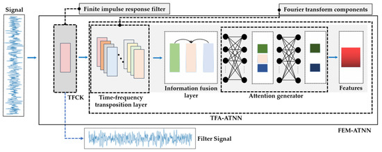
Figure 1.
A brief description of the method in this paper: firstly, TFCK is used to filter the raw signal; secondly, a set of convolution kernels are adopted to extract the time-frequency feature from the filtered signal; finally, an attention-based network is conducted to features.
2.1. Time-Domain Filter with Convolution Kernel
The FIR filter can retain the target signal and suppress the interference. It performs weighting processing on the continuous input signal, then obtains the filtered signal by accumulation. An Nth-order FIR filter multiplies N times and accumulates N-1 times to complete one filtering operation. This process is expressed as follows:
where and represent the output and input of the filter, denotes the filtering coefficient, and N denotes the order of the filter. As for one-dimensional convolution operations with convolution kernels of odd length, it can be expressed as:
where and denote the output and input of the 1D-CK, denotes the weight of the 1D-CK, N denotes the kernel size of the 1D-CK, s denotes the stride of the convolutional layer, denotes the bias, and denotes the activation function. Therefore, an FIR filter can be designed based on a single 1D-CK that the bias and activation function of it are removed. When the stride and kernel size of convolution are set to 1 and N, 1D-CK can be treated as a Nth-order FIR filter with a delay of . For the classification task, the FIR filter conducted by 1D-CK can be regarded as an adaptive filter or a fixed-parameter filter, which can be optimized parameters by gradient descent adaptively or filtered the raw signal according to fixed optimal parameters, named TFCK. TFCK is shown in Figure 2.
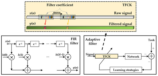
Figure 2.
The schematic diagram of TFCK.
The parameter design method of TFCK is the same as that of the traditional FIR filter. For a specific underwater acoustic target recognition task, TFCK can learn the filter’s frequency response by gradient descent. In other words, it can automatically search for the frequency range suitable for the current classification task from the data. The adjustment strategy of TFCK includes two stages: the pre-trained stage and the training stage. In the pre-trained stage, all parameters of 1D-CK are adaptively learned according to a specific classification task. By observing the feedback of the neural network, we can analyze the inner workings and behavior of the models, strengthen the extraction of high-value information and suppress the perception of noise by the neural network. In the training stage, we can adjust and fix the parameters of 1D-CK according to the feedback of the network in the pre-trained stage, optimize the ability of the neural network to suppress low-value information and make the subsequent network easier to learn the generalized embedding features. Two stages are shown in Figure 3.
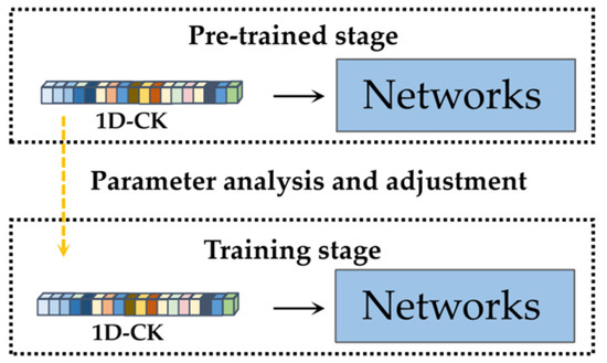
Figure 3.
Adjustment strategy of TFCK.
Figure 4 shows the frequency response of TFCK in the classification task of the ShipsEar [36] dataset.
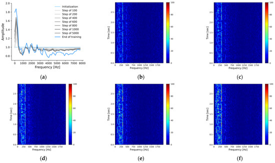
Figure 4.
The frequency response of TFCK and spectrograms of a filtered signal at a specific frequency band in the pre-trained stage. (a) The frequency response of TFCK; (b) Initialization; (c) The step of 100; (d) The step of 400; (e) The step of 1000; (f) End of training.
It can be seen that in the classification task of ShipsEar, TFCK is very sensitive to low-frequency information at the initial stage of training. The training process gradually amplifies the importance of low-frequency information, and the neural network finds several peaks with similar intervals. At the last stage of the training process, the perception of the neural network is finally stabilized within a range, and the redundant information for the current network architecture and the classification task is fed back. The high-frequency information of ship radiated noise is seriously lost through the underwater acoustic channel, and the low-frequency information can spread further in the underwater environment. Usually, the identifiable information from ship radiated noise received by the hydrophone is concentrated in the low-frequency of the raw signal. This result means that the knowledge of TFCK learned from the data is consistent with the cognition of experts in underwater acoustic target recognition, which is also the same as the objective laws of physics. According to the result, the differentiated information among categories in the data set is mainly concentrated below 600 Hz. Therefore, the parameters of TFCK can be optimized to complete the classification task better than before. The parameter of Equation (2) is set to (4), and the 1D-CK is set according to the traditional low-pass FIR filter of 1500 Hz cutoff frequency.
2.2. Time-Frequency Analysis Module of Attention-Based Neural Network
As a classical time-frequency analysis method, the short-time Fourier transform (STFT) can reflect the frequency change of ship radiated noise over time. Firstly, TFA-ATNN uses a set of 1D-CKs to embed the Fourier transform into the neural network, so that the neural network is able to extract time-frequency features. Secondly, the attention mechanism is conducted to improve the perception ability of the neural network for frequency. Discrete Fourier transform (DFT) can decompose frequency components from complex time-domain waveforms and is an important method for signal analysis and processing. In this paper, DFT is realized based on 1D-CK. DFT can be expressed as Equations (3) and (4):
where denotes the time-domain signal sequence, and the discrete Fourier transform and its inverse transform are and . In order to realize the discrete Fourier transform by convolution neural layer, Equation (3) is expressed in matrix form, as follows:
where is used to replace . In addition, according to the Euler formula, Equation (3) can be decomposed into the representation of an imaginary component and a real component. The decomposition is as follows:
The typical convolutional neural network layer is represented by Equation (7):
where represents the output feature, represents the convolution kernel, represents the feature set, represents the bias, denotes the convolution kernel number, denotes the layer number, and is the convolution operation of the convolutional neural network. In particular, for the one-dimensional convolution layer that only inputs single-channel time series signals, when the length of the input signal and the convolution kernel are equal and the bias, activation function and padding are removed, Equation (7) can be transformed into Equation (8):
where represents the output of the convolution kernel, represents the input signal, and represents the weight of the convolution kernel. In order to realize the Fourier transform, we set two groups of convolution kernels to calculate the imaginary component and real component of the Fourier transform, respectively. The weights of these two groups of convolution kernels can be fixed according to the sine basis functions and cosine basis functions in Equation (6). The number of convolution kernels is constrained by the number of points in the Fourier transform, and it is also equal to the number of points in the Fourier transform divided by two and plus one. Therefore, a one-dimensional convolution layer based on removing bias, activation function and padding can realize Fourier transform operation. Furthermore, the STFT with different time resolution and frequency resolution can be realized by optimizing the size, step length and basis function of the convolution kernel, as shown in Figure 5. This module is called the basic STFT module based on the convolutional neural network (BSTFT-CNN). In addition, in order to attenuate sidelobe height and weaken the impact of spectrum leakage, Hanning window action on convolution kernels. Specifically, the Hanning window with length M is expressed as Equation (9):
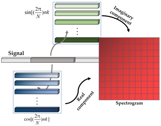
Figure 5.
The schematic diagram of the BSTFT-CNN.
Since the parameters of convolution kernels in the BSTFT-CNN are initialized by the standard sine basis functions and cosine basis functions, the network after the BSTFT-CNN will learn the frequency components extracted by the BSTFT-CNN indiscriminately. However, there are obvious frequency domain characteristics in ship radiated noise. The attention module of the short-time Fourier transform adopts the full connection layer with shared parameters (FCSP), hoping that the neural network can learn to automatically fuse the stable frequency components in the input signal and achieve a more stable recognition effect than before. This paper embeds an attention mechanism into the BSTFT-CNN to construct a convolution neural network time-frequency feature extraction module with an attention mechanism, which is called TFA-ATNN, as shown in Figure 6. The TFA-ATNN adopts the FCSP, hoping that the neural network will automatically extract the stable frequency components in the input signal to improve the stability of the recognition algorithm.
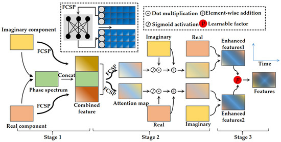
Figure 6.
The schematic diagram of TFA-ATNN.
The TFA-ATNN is mainly divided into three stages. In stage 1, the TFA-ATNN uses two FCSPs to learn the information that stably exists in the imaginary or real component and combine the components and phase spectrum as a combined features. In stage 2, the FCSP is used to fuse the combined feature. Feature fusion generates two attention maps, which are used for enhancement of imaginary and real components, respectively. In the last stage, a learnable factor is used to combine the enhanced spectrum generated by the result of enhancement. Finally, the combination result is the output features that could be sent to the network for embedding and extracting.
Specifically, the size of one of the component outputs by the BSTFT-CNN is , where is the number of time points and is the number of frequency points. In order to make it easier for the model to capture the stable frequency distribution, FCSP is proposed to constrain the relationship between frequency components. Its operation is expressed as Equation (10):
where is one of the output features of the BSTFT-CNN, which includes features of real components and imaginary components. is the parameter matrix of the FCSP, and its size is in stage 1, which depends on input and output. is the matrix output by the FCSP. represents the imaginary component, represents the real component, and subscript 1 represents stage 1. The number of neural units in the single layer of the FCSP is equal to the number of frequency points.
In stage 2, the TFA-ATNN combines the imaginary component, the real component and the phase component together, which is different from the classical attention mechanisms, such as SENet [37] and CBAM [38], to obtain attention information from the current layer to ensure that the model has sufficient information to extract the relationship between frequency components. The feature matrix is fused by concat, and the fused matrix is called . After the is obtained, it is input into the FCSP of stage 2, as in Equation (11):
where is the gate function, here it is sigmoid. dot multiplication to get , which is called the enhancement imaginary component. dot multiplication to get , called the enhancement real component. Finally, the weight factor with learning ability is used to fuse enhanced spectrums of the real and imaginary components. It is convenient for the neural network to initialize the weights of attention mechanisms adaptively according to tasks and parameters. Equation (12) describes the enhancement process:
where denotes the features extracted by the TFA-ATNN. Except for the parameters in the BSTFT-CNN, all parameters in the TFA-ATNN are adjusted during the training stage. The parameters that can be adjusted during the training stage in the TFA-ATNN are presented in Table 1.

Table 1.
Parameters of TFA-ATNN.
3. Deployment of Underwater Acoustic Target Recognition Network and Validation of Model Based Transfer Learning
Deep learning is a data-driven technique where training is performed on datasets and the trained models can be used to handle specific tasks. Data is scarce for the underwater acoustic target recognition task, especially in specific application scenarios. Training the model initialized by random parameters on scarce data always limits the model’s performance. Initializing the model with pre-trained parameters may improve the model’s performance, but this improvement depends on the size, type of pre-trained data, and the way transfer learning is done. The improper use of the pre-trained model will introduce negative optimization, resulting in a decline in performance. In audio pattern recognition, many researchers are exploring the effectiveness of the pre-trained model.
Inspired by Large-Scale Pretrained Audio Neural Networks (PANNs) [39], we conducted experiments to verify the applicability of the pre-trained model of the audio pattern recognition task in the underwater acoustic target recognition task. This paper transfers the audio pattern recognition model trained on large-scale data (AudioSet [40]) to an underwater acoustic target recognition task. Firstly, a strong audio pattern recognition model is trained under the condition of large-scale audio pattern recognition data. Then, the pre-trained model is transferred to the underwater acoustic target recognition task. Specifically, the parameters of the underwater acoustic target recognition model are initialized by using the parameters of the audio pattern recognition model. Finally, the transferred underwater acoustic target recognition model is trained on a specific underwater acoustic signal dataset. A typical deep neural network for classification is usually composed of two parts. The first part is the backbone network (Backbone) for extracting high-level features, including convolutional neural networks (CNN), transformers, time-delay neural networks (TDNN), etc. The other part is the neural network used for classification, and the fully connected network (FC) is a classic classification neural network. In order to improve the high-level feature extraction performance of neural networks, this paper implements model-based transfer learning on the backbone network. The schematic diagram of the model-based transfer learning strategy in this paper is shown in Figure 7.
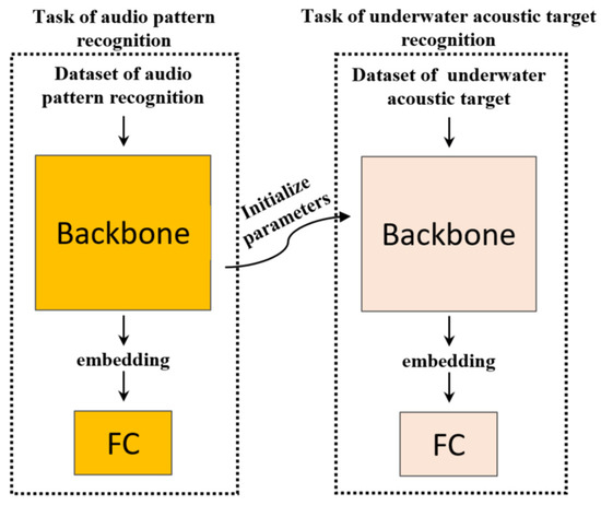
Figure 7.
The schematic diagram of model based transfer learning strategy.
The Visual Geometry Group (VGG) of Oxford University has proposed a backbone network with superior feature extraction performance called VGGNet [41]. The backbone network performs superiorly in image recognition, semantic segmentation, speech processing and other fields. Since then, researchers have applied VGGNet as a feature extractor to large-scale audio event detection tasks and achieved excellent results [40,42], called VGGish. In terms of model selection of the backbone network, this paper designs two backbones based on VGGish. VGGish is composed of continuously stacked convolution kernels, which have strong feature extraction performance and are easy to implement and expand. Typically, algorithms implemented on the VGGish can easily embed other deep learning techniques to further improve performance. Therefore, VGGish is suitable as the backbone for algorithm performance verification. In this paper, we use a pre-trained model to initialize the parameters in the backbone, and only initialize the common layers when the layers of different backbones are not completely consistent, to further ensure the versatility of the algorithm. The method and parameters of pre-training according to PANNs. Backbone 1 and Backbone 2 are shown in Table 2. In the convolutional layer, the C(64,3,1) means that there are 64 convolution kernels, the size of each is 3 × 3, and the stride is 1. Avg-pooling(1,2) means that the average pooling is 1 × 2.
Table 2.
Backbones are used in this paper.
After embedding feature extraction of Backbone, the full connected neural network is used as the classifier to classify the target. The fully connected network structures of Backbone 1 and Backbone 2 are almost identical, with only slight differences in parameters, as shown in Table 3. In Table 3, FC(512,256) means that the input size is 512 and the output size is 256. The x means the number of categories of classified tasks. Connect Backbone 1 and Classifier 1 to construct Network 1, and connect Backbone 2 and Classifier 2 to construct Network 2. In the training stage of the networks, the classifiers’ parameters are not initialized with pre-trained parameters, and all parameters need to be adjusted.
Table 3.
Classifiers are used in this paper.
4. Experiments and Discussion
4.1. Experimental Dataset
This paper conducts experiments on ShipsEar that consist of recordings from different regions of the Spanish Atlantic coastline in northwestern Spain during the autumn of 2012 and the summer of 2013, most of the data was collected at Porto Vigo (42°14.5′ N 008°43.4′ W) or nearby. The Port of Vigo is located within the Vigo River, a submerged river valley 35 km long, 10 km wide at its widest point, and has a maximum depth of less than 45 m. The recording equipment is the Hyd SR-1 hydroacoustic recorder. The core of this recorder is a hydrophone with a sensitivity of −193.5 dB re 1 V/1 uPa and a frequency response range of 1 Hz–28 kHz.
Vigo port is one of the largest fishing ports in the world, and there is a huge flow of fishing vessels on the waterway. The data-target categories collected in this area are diverse. Researchers deploy the hydrophones under the water and schedule labels according to vessel movement information obtained from the port authority and the Automatic Identification System for vessels. Original recordings were clipped to preserve information from the beginning to the end of the event or pass-by. ShipsEar comes from these edited recordings, which included 90 recordings in wav format lasting from 15 s to 10 min. The recordings contain 11 types of ship radiated noise signals, of which types of ship radiated noise signals can be divided into five categories based on vessel size according to [36], as is shown in Table 4. Each recording of ShipsEar contains only one type of vessel. The records in different recordings may come from different voyages, even if they are the same vessel type.
Table 4.
Target category on ShipsEar.
4.2. Experimental Methods
This section describes the experimental design and experimental details. This paper proposed FEM-ATNN to improve the underwater acoustic target recognition model’s accuracy, robustness and generalization. In addition, we verify the feasibility of applying the audio data pre-trained model to underwater acoustic target recognition. Due to the diversity in the speed of vessels, environment and navigation states, there are differences in ship radiated noise under different voyages. In short, the difference in radiated noise is closely related to the voyage. The difference in radiated noise at the beginning and end of a long-term voyage is greater than that in a short period. The difference in radiation noise between different voyages is more likely than that of the same voyage. For an intelligent system, the greater the difference between training and test data, the more generalized the model will be. Generally speaking, there are three ways to divide training data and test data: random segmentation, front/back segmentation, and different recording segmentation. Three types of division represent three different task difficulties, from simple to challenging. The method of evenly segmenting the recordings and randomly selecting the training set and test set may obtain high accuracy, but it is too easy and cannot well evaluate the underwater acoustic target recognition algorithm because the training data and test data are highly similar in the near seconds. Therefore, this paper designs two classification tasks according to front/back segmentation and different recording segmentations based on ShipsEar, selects 88 recordings for experiments, and both tasks divide recordings into five categories according to Table 4. Task 1 is to construct a fourfold dataset by dividing each of the recordings into four pieces on average according to the time sequence. This division method can separate training data and test data to a certain extent, which is suitable for evaluating the fitting ability of the neural network model. Arranging each recording as training or test data in a 3-1 ratio is Task 2. Task 2 is difficult because the underwater acoustic target recognition algorithm should be able to identify the unknown voyages even if the specific target is not present in the training set. Task 2 is more suitable for evaluating the algorithm’s generalization and practicability than Task 1. We use Network 1 in Task 1 and conduct Network 2 in Task 2. All data is downsampled to 16 kHz, and 3626 records of data are obtained through division and simple selection, and the duration of each data point is 3 s.
Based on two classification tasks, this paper arranges four groups of results comparisons to evaluate the proposed method’s performance. The first results compare the FEM-ATNN with multi-resolution STFT on task 2. The second experiment uses standard STFT as the primary feature to verify the performance of model-based transfer learning on task 1. The third experiment conducts the FEM-ATNN and model-based transfer learning in the same model, evaluates it on Task 1 and Task 2, and compares it with Mel filter bank energy (FBank), Mel frequency cepstral coefficients (MFCC) and linear frequency cepstral coefficients (LFCC). The last group of results compares the proposed method with other methods using ShipsEar in recent years. All the networks are trained by random gradient descent. Adam is used as the optimizer. The training minibatch is set to 32, the initial learning rate is set to 0.005, and the learning rate is decreased once every 5000 steps. The decline factor is 0.1, and a total of 15,000 steps are trained. The extraction methods of FBank, MFCC and LFCC refer to torchaudio [43]. FBank extracted with window size 2048 and hop length 1024. For FBank, the number of Mel filters is 128, followed by a logarithmic operation to extract input features. STFTs also utilize a logarithmic operation to extract input features in the training stage. For MFCC and LFCC, the number of mfc coefficients is set to 40, the number of linear filters is set to 128 and the number of lfc coefficients is set to 40. The convolution kernel size of TFCK is set to 63 as a low-pass FIR filter with a 1500 Hz cutoff frequency, and the parameters are locked in the training stage. The kernel size and strides of FEM-ATNN are set to 1024 and 512, respectively. Finally, we use recognition accuracy, recall rate, accuracy, and F1-score to evaluate the performance of the network.
4.3. Experimental Results and Discussion
This paper proposed a time-frequency analysis method based on neural networks, and our calculation process and implementation were derived from the original Fourier transform. Therefore, the first experiment in this paper compares the proposed method with the short-time Fourier transform method to consider the advantages of the proposed method. The STFTs with different parameters carry different information because STFTs with different parameters have different frequencies and time resolutions. It can be predicted that different pieces of information will lead to different final recognition performances. Therefore, this paper selects the STFT of a series of typical parameters for comparison to evaluate the performance of the proposed method. Experiment 1 is carried out on the most challenging Task 2 to evaluate the generalization of various methods. The STFT with multi-resolutions as the primary feature is extracted to the same backbone network, and the classification performance of these primary features is compared with the model based on the FEM-ATNN. The window length of STFTs is from 512 to 8192, and the hop length is set to half of the window length. Table 5 shows the result of experiment 1.
Table 5.
Recognition results of the FEM-ATNN and the multi-resolution STFT.
The STFT with different resolutions shows different performances in Experiment 1. Among them, the STFT has the best performance, with a window length of 2048. Its accuracy rate reaches 78.0%, which is significantly higher than others, especially compared with the window lengths of 4096 and 8192. The accuracy of the FEM-ATNN reaches 83.9%, which is 9.1%, 8.4%, 5.9%, 14.8% and 15.9% higher than the STFT with windows lengths from 512 to 8192, respectively.
Experiment 2 verifies the feasibility of transferring the model, which is pre-trained on the large-scale audio pattern recognition data, to the underwater acoustic target recognition task. The advantage of transfer learning is to transfer knowledge from other fields to the current field. For a simple task with little difference between training data and test data, the effect is often not noticeable. Therefore, we not only use tasks with differences between training data and test data but also evaluate the boundary performance of model-based transfer when the training data and test data are similar. Task 1 provides a variety of test data and training data combinations, so we conduct experiments on Task 1 to facilitate a complete evaluation of the algorithm’s performance. Task 1 divides each recording into four folds in chronological order. The differences between different folds and folds are not consistent. In other words, it is more challenging to use the head fold as the test set than the middle fold as the test set because the test data cut from the middle of the recordings is more similar to the surrounding training data. In order to evaluate it objectively, we used standard STFT as the primary feature in this experiment to compare the performance between the pre-trained and the random models. STFT-2048 is input into the backbone network as the primary feature because it is performed best in Task 2. The results of Experiment 2 are shown in Table 6.
Table 6.
Recognition results of model based transfer learning.
Table 6 shows the performance of the backbone network using pre-trained model parameter initialization and random initialization. The results show that model-based transfer learning can improve performance most of the time. The pre-trained model parameters can be used to initialize the backbone of the underwater acoustic target recognition model when the backbone is pre-trained on large-scale audio data unrelated to underwater acoustics. It is worth noting that the number of layers of the backbone used for underwater acoustic target recognition is different from that of the pre-trained backbone. We extract some layer parameters from the pre-training model to initialize all the layer parameters of the underwater acoustic target recognition backbone. That is, partial layer parameters are extracted from the pre-training model to initialize all layer parameters of the underwater acoustic target recognition network. The simple method effectively improves the recognition performance.
The previous experiments proved the effectiveness of the proposed method and the feasibility of model migration, but the experiments were evaluated independently. Experiment 3 was devoted to the model-based transfer to the FEM-ATNN-based model (FEM-ATNN-trans) and conducted experiments on Task 1 and Task 2. In addition, the STFT is only a fundamental time-frequency analysis method used in Experiment 1. Experiment 3 added other mainstream time-frequency analysis methods to the comparison, including MFCC, LFCC and FBank. The backbone of those methods is consistent with the FEM-ATNN-based model according to Task 1 and Task 2. The details of those features are described in the second paragraph of the Experimental Method section. The results are shown in Table 7.
Table 7.
Recognition results of proposed method and methods based on mainstream primary features.
For Task 1, fold 1 and fold 2 are selected for the experiment because they are the representative subtasks in Task 1, according to challenges. They represent the most challenging subtasks and the simplest subtasks in Task 1, as shown in Experiment 2. The test data of fold 1 is in the front of each recording, and the test data of fold 2 is in the middle. The difference between the test data and the training data of fold 2 is smaller than that of fold 1.
Although the subtask based on fold 2 is easier to achieve high accuracy than the subtask based on fold 1, it is still meaningful to experiment on the subtask based on fold 2. An overfitting algorithm may achieve high accuracy in simple tasks and show decadence in challenging tasks. Conversely, the model with solid generalization may perform both on complex and simple tasks because it has learned the high-level representation that can distinguish categories. As shown in Table 7, the FEM-ATNN-trans is superior to other methods in all tasks, especially in Task 2. The challenge of Task 2 is that it requires the algorithm to learn adequate generalization information from training data, which must meet the needs of the underwater acoustic target recognition task. In addition, the accuracy of the FEM-ATNN-trans is 3.9% higher than that of the FEM-ATNN in Table 5, which further verifies the effectiveness of the proposed method and model-based transfer learning.
Furthermore, we compare the FEM-ATNN-trans with other existing methods that have used the ShipsEar dataset, as shown in Table 8. Accuracy is used as a comparative measure because most papers use it to compare their results. The baseline is a machine learning method proposed in the ShipsEar research [36] with an accuracy of 75.4%. The accuracy of our method is the result of the representative subtask of Task 1, according to Table 7.
Table 8.
Comparison between the proposed method and other methods used ShipsEar.
The methods in Table 8 show studies in recent years, and our method shows competitive performance. On the one hand, most of the methods in Table 8 segment the recordings and randomly sample the adjacent segments as the train or test data, which is lower in classification difficulty than Task 1 used in this paper. On the other hand, some methods in the table adopt data augmentation technology, such as methods of No.7 and No.8, which both used SpecAugment. The FEM-ATNN-trans does not use data augmentation technology but still performs well.
5. Conclusions
In this paper, a time-frequency feature extraction module based on the attention mechanism neural network is proposed, which combines the operation mechanism of the convolutional neural network, time-domain filtering and Fourier transform. The proposed method can extract the input time domain signal directly, which is an end-to-end training model. Classic deep learning methods search for features through neural networks such as black-box models, and it is difficult for researchers to analyze the inner workings and behavior of the models. The proposed method can output the frequency domain response of the neural network in real-time. It is convenient for researchers to understand the neural network learning process, which helps to strengthen the network model and improve its generalization. In addition, the feasibility of transferring non-underwater acoustic data as pre-trained data to underwater acoustic target recognition is verified. A series of classification experiments demonstrate the effectiveness of the proposed method, especially for tasks with a demand for model generalization ability.
Author Contributions
Conceptualization, D.L. and F.L.; methodology, D.L.; software, F.L. and D.L.; validation, T.S., D.Z. and L.C.; resources, T.S.; investigation, D.Z.; writing—original draft preparation, X.Y. and D.L.; writing—review and editing, X.Y. and L.C.; supervision, T.S. All authors have read and agreed to the published version of the manuscript.
Funding
This research received no external funding.
Institutional Review Board Statement
Not applicable.
Informed Consent Statement
Not applicable.
Data Availability Statement
Data available in a publicly accessible repository. The data presented in this study are openly available in available at 10.1016/j.apacoust.2016.06.008 in ref [36].
Conflicts of Interest
The authors declare no conflict of interest.
References
- Meng, Q.; Yang, S.; Piao, S. The classification of underwater acoustic target signals based on wave structure and support vector machine. J. Acoust. Soc. Am. 2014, 136, 2265. [Google Scholar] [CrossRef]
- Meng, Q.; Yang, S. A wave structure based method for recognition of marine acoustic target signals. J. Acoust. Soc. Am. 2015, 137, 2242. [Google Scholar] [CrossRef]
- Jiang, J.; Wu, Z.; Lu, J.; Huang, M.; Xiao, Z. Interpretable features for underwater acoustic target recognition. Measurement 2020, 173, 108586. [Google Scholar] [CrossRef]
- Lourens, J. Classification of ships using underwater radiated noise. In Proceedings of the COMSIG 88@ m_Southern African Conference on Communications and Signal Processing, Pretoria, South Africa, 24 June 1989; pp. 130–134. [Google Scholar] [CrossRef]
- Rajagopal, R.; Sankaranarayanan, B.; Rao, P.R. Target classification in a passive sonar-an expert system ap-proach. In Proceedings of the International Conference on Acoustics, Speech, and Signal Processing, Albuquerque, NM, USA, 3–6 April 1990; pp. 2911–2914. [Google Scholar] [CrossRef]
- Ferguson, B.G. Time-frequency signal analysis of hydrophone data. IEEE J. Ocean. Eng. 1996, 21, 537–544. [Google Scholar] [CrossRef]
- Boashash, B.; O’Shea, P. A methodology for detection and classification of some underwater acoustic signals using time-frequency analysis techniques. IEEE Trans. Acoust. Speech Signal Process. 1990, 38, 1829–1841. [Google Scholar] [CrossRef]
- Liu, J.; He, Y.; Liu, Z.; Xiong, Y. Underwater Target Recognition Based on Line Spectrum and Support Vector Machine. In Proceedings of the 2014 International Conference on Mechatronics, Control and Electronic Engineering (MCE-14), Shenyang, China, 29–31 August 2014. [Google Scholar] [CrossRef]
- Ou, H.; Allen, J.S.; Syrmos, V.L. Automatic classification of underwater targets using fuzzy-cluster-based wavelet signatures. J. Acoust. Soc. Am. 2009, 125, 2578. [Google Scholar] [CrossRef]
- Huang, Q.; Azimi-Sadjadi, M.R.; Tian, B.; Dobeck, G. Underwater target classification using wavelet packets and neural networks. In Proceedings of the 1998 IEEE International Joint Conference on Neural Networks Proceedings. IEEE World Congress on Computational Intelligence, Anchorage, AL, USA, 4–9 May 2002. [Google Scholar] [CrossRef]
- Zeng, X.-Y.; Wang, S.-G. Bark-wavelet Analysis and Hilbert–Huang Transform for Underwater Target Recognition. Def. Technol. 2013, 9, 115–120. [Google Scholar] [CrossRef]
- Jahromi, M.S.; Bagheri, V.; Rostami, H.; Keshavarz, A. Feature Extraction in Fractional Fourier Domain for Classification of Passive Sonar Signals. J. Signal Process. Syst. 2019, 91, 511–520. [Google Scholar] [CrossRef]
- Tucker, S. Auditory Analysis of Sonar Signals. Ph.D. Thesis, University of Sheffield, Britain, UK, 2001. [Google Scholar]
- Zhang, L.; Wu, D.; Han, X.; Zhu, Z. Feature Extraction of Underwater Target Signal Using Mel Frequency Cepstrum Coefficients Based on Acoustic Vector Sensor. J. Sensors 2016, 2016, 1–11. [Google Scholar] [CrossRef]
- Wang, S.; Zeng, X. Robust underwater noise targets classification using auditory inspired time–frequency analysis. Appl. Acoust. 2014, 78, 68–76. [Google Scholar] [CrossRef]
- Li-Xue, Y.; Ke-An, C.; Bing-Rui, Z.; Yong, L. Underwater acoustic target classification and auditory feature identification based on dissimilarity evaluation. Acta Phys. Sin. 2014, 63, 134304. [Google Scholar] [CrossRef]
- Mohankumar, K.; Supriya, M.H.; Pillai, P.S. Bispectral Gammatone Cepstral Coefficient based Neural Network Classifier. In 2015 IEEE Underwater Technology (UT); IEEE: Piscataway, NJ, USA, 2015; pp. 1–5. [Google Scholar] [CrossRef]
- Hemminger, T.; Pao, Y.-H. Detection and classification of underwater acoustic transients using neural networks. IEEE Trans. Neural. Netw. 1994, 5, 712–718. [Google Scholar] [CrossRef] [PubMed]
- Yang, H.; Gan, A.; Chen, H.; Pan, Y.; Tang, J.; Li, J. Underwater acoustic target recognition using SVM ensemble via weighted sample and feature selection. In Proceedings of the 2016 13th International Bhurban Conference on Applied Sciences and Technology (IBCAST), Islamabad, Pakistan, 12–16 January 2016; pp. 522–527. [Google Scholar] [CrossRef]
- Doan, V.-S.; Huynh-The, T.; Kim, D.-S. Underwater Acoustic Target Classification Based on Dense Convolutional Neural Network. IEEE Geosci. Remote Sens. Lett. 2022, 19, 3029584. [Google Scholar] [CrossRef]
- Hu, G.; Wang, K.; Liu, L. Underwater Acoustic Target Recognition Based on Depthwise Separable Convolution Neural Networks. Sensors 2021, 21, 1429. [Google Scholar] [CrossRef] [PubMed]
- Tian, S.; Chen, D.; Wang, H.; Liu, J. Deep convolution stack for waveform in underwater acoustic target recognition. Sci. Rep. 2021, 11, 1–14. [Google Scholar] [CrossRef]
- Cao, X.; Togneri, R.; Zhang, X.; Yu, Y. Convolutional Neural Network With Second-Order Pooling for Underwater Target Classification. IEEE Sensors J. 2018, 19, 3058–3066. [Google Scholar] [CrossRef]
- Li, C.; Liu, Z.; Ren, J.; Wang, W.; Xu, J. A Feature Optimization Approach Based on Inter-Class and Intra-Class Distance for Ship Type Classification. Sensors 2020, 20, 5429. [Google Scholar] [CrossRef]
- Yang, H.; Xu, G.; Yi, S.; Li, Y. A New Cooperative Deep Learning Method for Underwater Acoustic Target Recognition. In OCEANS 2019-Marseille; IEEE: Piscataway, NJ, USA, 2019; pp. 1–4. [Google Scholar] [CrossRef]
- Zhang, Q.; Da, L.; Zhang, Y.; Hu, Y. Integrated neural networks based on feature fusion for underwater target recognition. Appl. Acoust. 2021, 182, 108261. [Google Scholar] [CrossRef]
- Wang, X.; Liu, A.; Zhang, Y.; Xue, F. Underwater Acoustic Target Recognition: A Combination of Multi-Dimensional Fusion Features and Modified Deep Neural Network. Remote Sens. 2019, 11, 1888. [Google Scholar] [CrossRef]
- Luo, X.; Feng, Y.; Zhang, M. An Underwater Acoustic Target Recognition Method Based on Combined Feature With Automatic Coding and Reconstruction. IEEE Access 2021, 9, 63841–63854. [Google Scholar] [CrossRef]
- Liu, F.; Shen, T.; Luo, Z.; Zhao, D.; Guo, S. Underwater target recognition using convolutional recurrent neural networks with 3-D Mel-spectrogram and data augmentation. Appl. Acoust. 2021, 178, 107989. [Google Scholar] [CrossRef]
- Kamal, S.; Mujeeb, A.; Supriya, M.H. Generative adversarial learning for improved data efficiency in underwater target classification. Eng. Sci. Technol. 2022, 30, 101043. [Google Scholar] [CrossRef]
- Raissi, M.; Perdikaris, P.; Karniadakis, G. Physics-informed neural networks: A deep learning framework for solving forward and inverse problems involving nonlinear partial differential equations. J. Comput. Phys. 2019, 378, 686–707. [Google Scholar] [CrossRef]
- Shahbazi, A.; Monfared, M.S.; Thiruchelvam, V.; Fei, T.K.; Babasafari, A.A. Integration of knowledge-based seismic inversion and sedimentological investigations for heterogeneous reservoir. J. Southeast Asian Earth Sci. 2020, 202, 104541. [Google Scholar] [CrossRef]
- Chen, Y.; Lu, L.; Karniadakis, G.E.; Negro, L.D. Physics-informed neural networks for inverse problems in nano-optics and metamaterials. Opt. Express 2020, 28, 11618–11633. [Google Scholar] [CrossRef]
- Khayer, K.; Kahoo, A.R.; Monfared, M.S.; Tokhmechi, B.; Kavousi, K. Target-Oriented Fusion of Attributes in Data Level for Salt Dome Geobody Delineation in Seismic Data. Nonrenewable Resour. 2022, 31, 2461–2481. [Google Scholar] [CrossRef]
- Deng, J.; Dong, W.; Socher, R.; Li, L.-J.; Li, K.; Fei-Fei, L. ImageNet: A large-scale hierarchical image database. In Proceedings of the 2009 IEEE Conference on Computer Vision and Pattern Recognition, Miami, FL, USA, 20–25 June 2009; pp. 248–255. [Google Scholar] [CrossRef]
- Santos-Domínguez, D.; Torres-Guijarro, S.; Cardenal-López, A.; Pena-Gimenez, A. ShipsEar: An underwater vessel noise database. Appl. Acoust. 2016, 113, 64–69. [Google Scholar] [CrossRef]
- Hu, J.; Shen, L.; Sun, G. Squeeze-and-Excitation Networks. In Proceedings of the IEEE Conference on Computer Vision and Pattern Recognition (CVPR), Salt Lake City, UT, USA, 18–23 June 2018; pp. 7132–7141. [Google Scholar]
- Woo, S.; Park, J.; Lee, J.Y.; Kweon, I.S. CBAM: Convolutional block attention module. arXiv 2018, arXiv:1807.06521. [Google Scholar]
- Kong, Q.; Cao, Y.; Iqbal, T.; Wang, Y.; Wang, W.; Plumbley, M.D. PANNs: Large-Scale Pretrained Audio Neural Networks for Audio Pattern Recognition. IEEE/ACM Trans. Audio, Speech, Lang. Process. 2020, 28, 2880–2894. [Google Scholar] [CrossRef]
- Gemmeke, J.F.; Ellis, D.P.W.; Freedman, D.; Jansen, A.; Lawrence, W.; Moore, R.C.; Plakal, M.; Ritter, M. Audio Set: An ontology and human-labeled dataset for audio events. In Proceedings of the 2017 IEEE International Conference on Acoustics, Speech and Signal Processing (ICASSP), New Orleans, LA, USA, 5–9 March 2017; pp. 776–780. [Google Scholar] [CrossRef]
- Simonyan, K.; Zisserman, A. Very Deep Convolutional Networks for Large-Scale Image Recognition. arXiv 2014, arXiv:1409.1556. [Google Scholar]
- Hershey, S.; Chaudhuri, S.; Ellis, D.P.W.; Gemmeke, J.F.; Jansen, A.; Moore, R.C.; Plakal, M.; Platt, D.; Saurous, R.A.; Seybold, B.; et al. CNN architectures for large-scale audio classification. In Proceedings of the 2017 IEEE International Conference on Acoustics, Speech and Signal Processing (ICASSP), New Orleans, LA, USA, 5–9 March 2017; pp. 131–135. [Google Scholar] [CrossRef]
- Yang, Y.Y.; Hira, M.; Ni, Z.; Astafurov, A.; Chen, C.; Puhrsch, C.; Quenneville-Bélair, V. Torchaudio: Building Blocks for Audio and Speech Processing. In Proceedings of the 2022 IEEE International Conference on Acoustics, Speech and Signal Processing (ICASSP), Singapore, 22–27 May 2022; pp. 6982–6986. [Google Scholar] [CrossRef]
- Fernandes, R.P.; Apolinário, J.A., Jr. Underwater target classification with optimized feature selection based on Genetic Algorithms. SBrT 2020. [Google Scholar] [CrossRef]
- Xie, J.; Chen, J.; Zhang, J. DBM-Based Underwater Acoustic Source Recognition. In Proceedings of the 2018 IEEE International Conference on Communication Systems (ICCS), Chengdu, China, 19–21 December 2018; pp. 366–371. [Google Scholar] [CrossRef]
- Luo, X.; Feng, Y. An Underwater Acoustic Target Recognition Method Based on Restricted Boltzmann Machine. Sensors 2020, 20, 5399. [Google Scholar] [CrossRef] [PubMed]
- Yang, H.; Gu, H.; Yin, J.; Yang, J. GAN-based Sample Expansion for Underwater Acoustic Signal. J. Physics: Conf. Ser. 2020, 1544, 12104. [Google Scholar] [CrossRef]
- Hong, F.; Liu, C.; Guo, L.; Chen, F.; Feng, H. Underwater Acoustic Target Recognition with a Residual Network and the Optimized Feature Extraction Method. Appl. Sci. 2021, 11, 1442. [Google Scholar] [CrossRef]
- Khishe, M. DRW-AE: A Deep Recurrent-Wavelet Autoencoder for Underwater Target Recognition. IEEE J. Ocean. Eng. 2022, 47, 1083–1098. [Google Scholar] [CrossRef]


Publisher’s Note: MDPI stays neutral with regard to jurisdictional claims in published maps and institutional affiliations. |
© 2022 by the authors. Licensee MDPI, Basel, Switzerland. This article is an open access article distributed under the terms and conditions of the Creative Commons Attribution (CC BY) license (https://creativecommons.org/licenses/by/4.0/).