Abstract
Reflectance Transformation Imaging (RTI) is a non-contact technique which consists in acquiring a set of multi-light images by varying the direction of the illumination source on a scene or a surface. This technique provides access to a wide variety of local surface attributes which describe the angular reflectance of surfaces as well as their local microgeometry (stereo photometric approach). In the context of the inspection of the visual quality of surfaces, an essential issue is to be able to estimate the local visual saliency of the inspected surfaces from the often-voluminous acquired RTI data in order to quantitatively evaluate the local appearance properties of a surface. In this work, a multi-scale and multi-level methodology is proposed and the approach is extended to allow for the global comparison of different surface roughnesses in terms of their visual properties. The methodology is applied on different industrial surfaces, and the results show that the visual saliency maps thus obtained allow an objective quantitative evaluation of the local and global visual properties on the inspected surfaces.
1. Introduction
Mastering the functional properties of manufactured surfaces is a major scientific and industrial challenge for a wide variety of applications [1]. The functional properties of surfaces cover a large spectrum. A non-exhaustive list includes tribological properties [2,3], properties associated with material mechanics [4], wettability [5], biological properties, and functional parameters linked to light–surface interaction. This approach induces many issues and scientific challenges, in particular, the choice of measurement technology, the choice of the scale for both measurement and analysis tasks, and the choice of filtering and post-treatment methods. In this context, the RTI imaging method is currently experiencing significant growth [4,6,7] and is positioned as a complement to conventional techniques in industry, which are often based on 3D microscopy for the measurement of surface roughness.
During the RTI acquisition, the orientation of the light source varies around the surface and passes through a hemispherical space (constant distance). A fixed camera positioned orthogonally to the surface captures the response of the surface (local reflectance) for different lighting angles (angular reflectance). From the acquisition, N stereo-photometric type images are obtained, each pixel of which corresponds to a discrete measurement of the reflectance of the corresponding point on the surface, as shown in Figure 1, where and represent the components associated with the directions of illumination projected in the horizontal plane.
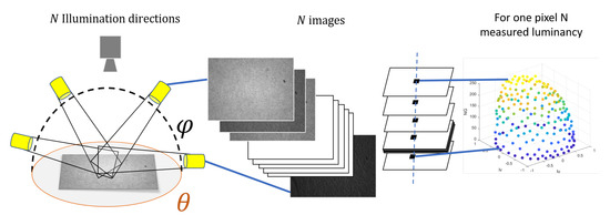
Figure 1.
Diagram of an RTI acquisition.
RTI was originally developed at HP labs by Malzbender et al. [8,9] under a name, Polynomials Texture Mappings (PTM), that refers to the implemented modeling method. Other modeling methods have been developed, such as the HSH (Hemispherical Harmonics) model [10,11,12,13], the DMD (Discrete Modal Decomposition) method [14,15,16,17], and the approach based on RBF (Radial Basis Function) [18,19]. Particularly important development has occurred in the field of the digitization of historical and cultural heritage objects [20,21,22]. More recently, this technique has been implemented in the context of a wide variety of industrial applications. These applications have often been related to the challenge of mastering of surface appearance perception and the automation of inspection processes [23,24], although other applications have been found in biomedicine, forensics [25], materials mechanics [4,26], and the analysis of tribological properties [17]. The richness of the contribution of the RTI technique is linked to the quality and variety of surface information that it can estimate. Indeed, this type of acquisition makes it possible to characterize the local angular reflectance of surfaces, i.e., the way light is re-emitted at each point as a function of the angle of illumination. Certain descriptors can statistically describe the angular reflectance response of a surface from RTI data (Figure 2). This type of information is particularly relevant for issues related to surface appearance quality [27], where the challenge lies in increasing the robustness of the results obtained from conventionally implemented sensorial analysis [28,29,30]. The RTI technique makes it possible to estimate characteristics linked to the local micro-geometry of surfaces, such as local descriptors of slopes, curvatures, and even topographic descriptors, through integration following the stereophotometric technique. In addition, the specularity and diffusion components provide access to sub-pixel light behaviors, as responses from multiple surface points can be integrated into a single pixel. Thus, we can observe the response of a point on the surface despite it being geometrically of a smaller size than the resolution of the sensor. RTI acquisition and characterization makes it possible to more directly measure and describe aspect function, i.e., the effect that is not geometry intrinsic and is instead created by the geometry of the surface [7,31].
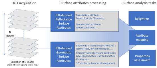
Figure 2.
Description of an RTI acquisition and the different types of descriptors.
Therefore, depending on the density of the acquisition angles and the methods chosen, RTI acquisition can lead to obtaining a voluminous and complex set of data [18,32,33]. Estimation of the descriptors constitutes a first step in data reduction, which allows a better understanding of the local surface characteristics and facilitates the analysis and post-processing carried out based on this type of acquisition. However, these descriptors vary in terms of unit, amplitude, and even dispersion; analyzed independently, they generally do not make it possible to match the various stakes of analysis in the context of controlling the appearance of manufactured surfaces. In this article, we propose a methodological contribution to answer this problem. The proposed method consists in locally (intra-surface) or globally (inter-surface) estimating the visual saliency from the data and descriptors extracted from RTI acquisitions.
Indeed, saliency maps aim to respond to an important issue for manufacturers, mentioned above, which is to allow better detection while assessing the criticality of aspect anomalies. In Section 2, we show how a multivariate and multi-scale analysis of the descriptors previously extracted from the RTI acquisitions can be used to determine the local saliency of the points/pixels of the inspected surface in an efficient way. This approach is then extended in Section 3 to the analysis of global anomalies, i.e., the mapping of the difference in appearance between one or more surface states and a reference surface state. These maps make it possible to functionally quantify the distance between two surfaces, i.e., in terms of overall appearance thereby meeting the challenge of managing the manufacturing and surface finishing processes, which require that differences in terms of appearance between surfaces be discriminated and evaluated.
2. Visual Saliency Estimation
The visual saliency of a pixel of an image corresponds to its ability to attract attention in relation to other points on the surface, in particular in relation to its neighbors. When observing a set, a human concentrates most of their perceptual and cognitive resources on the most salient subset. Therefore, estimation of visual saliency is an important issue in the analysis and characterization of the appearance of surfaces. The mapping of points with appearance attributes that are different from those of their environment and the quantification of these deviations are essentials that provide objective support for many surface inspection and analysis tasks. In the literature, an approach for calculating saliency from RTI data has already been proposed by Pitard et al. [16] based on the analysis of the Discrete Modal Decomposition coefficients, an experimental model for relighting. Here, we propose to extend this approach using the set of descriptors extracted from RTI data and to improve the performance of visual saliency estimation on multiple levels by taking multi-scale aspects into account in the calculation.
In order to illustrate the proposed methodology, we apply it to an application surface associated with the watch industry, specifically, a watch dial with a precious material deposit and a polished finish. Manufactured micro-scratches in known locations and with different geometric characteristics were made on the surface with a scratch test machine (Anton Paar ). The characteristics of this sample are shown in Figure 3. The acquisitions were carried out with a custom device consisting of a monochromatic two-thirds active pixel-type CMOS sensor with a resolution of 12.4 MPix () and a white uniform light (high power LED). In terms of RTI acquisition modalities, 149 angular positions distributed homogeneously in the angular space () were acquired, with an exposure time of 125 ms.
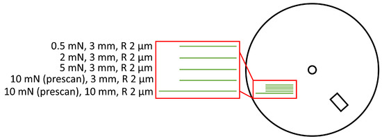
Figure 3.
Representation of the watch dial with standardized scratches. The red rectangle represents the acquisition zone.
2.1. Proposed Methodology
In order to identify and evaluate surface anomalies in the context of appearance quality control, it is necessary to be able to compare the points of the surface with each other using an objective criterion. A point is an anomaly when its behavior is different from its neighborhood or from the sought function. As the comparison cannot be absolute, only relative, this amounts to calculating distances between surface points. The distance, called the saliency in the case of intra-surface distances, is estimated from a multivariate analysis of the descriptors of the observed pixel descriptors Y relative to the average values of descriptors of the reference pixels X associated with the neighborhood under consideration. The method chosen here is based on the Mahalanobis distance [34], as illustrated in Figure 4, and is described in Equation (1) below:
where the matrix corresponds to the descriptor vectors of length k of n observation pixels and the matrix corresponds to the descriptor vectors of length k of m reference pixels used to estimate the distance. Here, and are respectively associated with the covariance matrix and the average of X over the dimension of the descriptors. During computation of the distance, the centering is performed on the dimension of the descriptors.
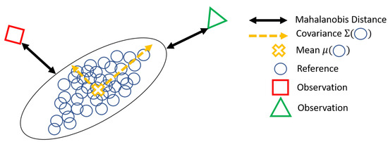
Figure 4.
Diagram of the Mahalanobis distance.
The Mahalanobis distance has the advantage of being a unitless and data scale-invariant multivariate method of analysis, and takes into account both the scatter and correlation of the data. Thus, several different unit and scale descriptors can be used when calculating the Mahalanobis distance, and the different descriptors can be weighted according to their respective dispersions. The choice of descriptors used when estimating saliency is important, as each allows the discrimination of different behaviors, which may potentially be antagonistic. Therefore, it is necessary to estimate which descriptors are the most relevant for characterizing a desired behavior, for example, a type of aspect abnormality, or to choose them based on experience or prior knowledge. An example is presented in Figure 5 highlighting the the significant difference in the saliency maps (monovaried in this case) depending on the choice of descriptor(s), here, the geometrics and the statistics descriptors, respectively, of the angular reflectance response.
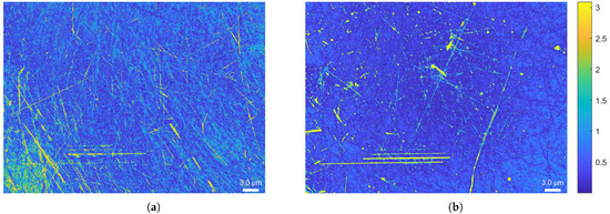
Figure 5.
Saliency maps derived from an RTI acquisition with an exposure time () of 125 ms on a polished watch dial with micro-scratches of different amplitudes: (a) Saliency from geometric descriptors and (b) Saliency from statistic descriptors.
2.2. Multi-Level Optimization Criterion
When estimating saliency, the most salient pixels sought are included among those used for reference. However, including salient pixels among the reference pixels can significantly modify the value of the descriptors. Depending on the case, the saliency estimated at each point can be over- or underestimated by the number and intensity of the salient points in the zone considered. For example, the salient points of the surface may have their saliency levels underestimated when are compared, in terms of distance, with points of the surface that have the same salience as themselves. If these points are salient, they probably have similar characteristics, and therefore similar descriptors. On the other hand, the non-salient points of the surface have their saliency levels increased because, althoough their characteristics are far from the salient ones, they are used as a reference. To overcome this problem, we propose the level factor saliency optimization method described in Equation (2). This method allows both the standard deviation and the mean of the saliency of the reference pixels used for the saliency computation to be reduced by removing the outliers (high saliency values). The method, which is illustrated in Figure 6, begins with an initialization step in which the saliency of the pixels studied must be estimated for the first time. A percentage of pixels is then removed based on the deviation from the mean of a distribution of points considered to be normal, corresponding to the most salient points of the reference pixels, before iterating the calculation of the distance with the remaining reference pixels.
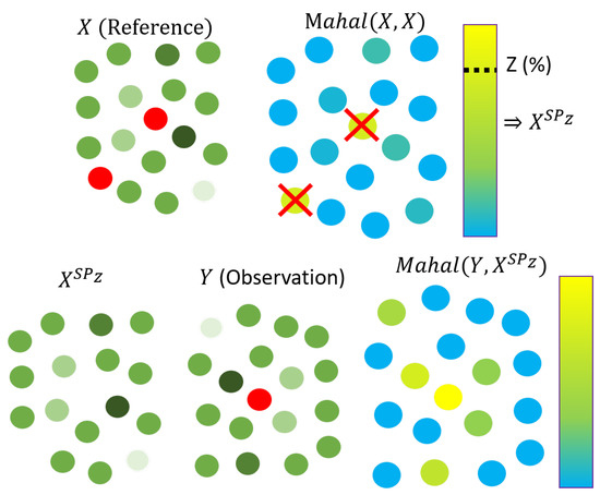
Figure 6.
Diagram of level factor visual saliency.
The percentage of pixels to remove is a parameter of the method, and is defined by the user beforehand. This parameter can be defined automatically to ensure that the standard deviation or the mean of the saliency of the reference pixels is close to a desired value. Figure 7 shows the effect of the choice of the percentage when using the level factor saliency estimation method; the higher the percentage, the greater the dynamics of the saliency. This increase in dynamics allows better visual observation of surface anomalies on the saliency maps, and helps with the segmentation and classification of surface anomalies.
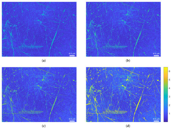
Figure 7.
Level factor saliency map estimated with the statistics descriptors calculated from an RTI acquisition of a watch dial with micro-scratches: (a) Saliency map ; (b) Saliency map ; (c) Saliency map ; (d) Saliency map .
Level factor saliency filters out salient pixels with a certain percentage. Moreover, it is possible to compress the saliency information from several level factors into a single saliency called the multi-level saliency. Multi-level saliency is computed from the weighted sum of differents factor levels of saliency, as described in the Equation (3). In our case, the weight of a level factor saliency corresponds to its entropy in order to take into account the disparity of the saliency information [35]. The results of multi-level saliency can be seen in Figure 8.
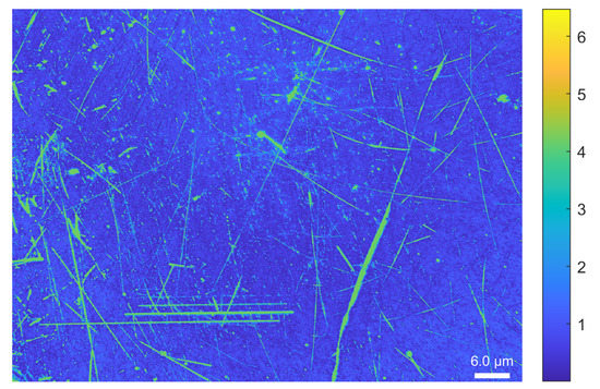
Figure 8.
Multi-level saliency map estimated with the statistics descriptors calculated from an RTI acquisition of the watch dial: Saliency map multi-level , , , .
2.3. Multi-Scale Saliency
The estimation of the visual saliency of a point on the surface depends on the points used as reference, and in particular on the possible presence of salient points in the reference considered, as mentioned in the previous section. Another important parameter is the scale of observation, which is even more the case when analysing the appearance of surfaces, where it is well known that scale effects are particularly important in perception. Thus, an anomaly may appear more or less salient when the surface is observed locally or as a whole, and the saliency must therefore integrate these scale factors. For example, many small and weak surface anomalies can be attenuated by the presence of large anomalies in the neighbors or their presence among the reference surface points. Conversely, changing the scale of observation by varying the size of the neighborhood around the calculation point can increase the saliency value of the weakest anomalies and facilitate their detection/evaluation. The calculation of the scale factor saliency makes it possible to solve this problem using a sliding window, as described in Equation (4) and illustrated in Figure 9.
where corresponds to the sliding window centered on pixel of size pixels and are the coordinates of the pixels in the sliding window.
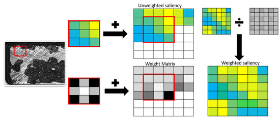
Figure 9.
Diagram of scale factor visual saliency.
At each sliding window position, the saliency of the points contained in the window is calculated by taking these same points as a reference. However, in order to take into account that the salience varies with the distance from the considered neighborhood, the calculation is weighted using a 2D Gaussian function, thus allocating more weight in the estimation of the salience to the points close to the calculation point. At each saliency calculation, a weight matrix is filled with the Gaussian function when moving the sliding window. The different parameters of the algorithm are then the size of the window , the translation step of the window , and the standard deviation of the Gaussian function .
The result of the scale factor salience can be seen in Figure 10. It can be seen that the number of small anomalies increases when the size of the sliding window decreases. Moreover, we observe that the area and the level of salience of anomalies detected with a small window seems to decrease. This reduction is due to the proportionality (or not) of salient points inside the sliding window. Indeed, when taking the whole of the surface, the surface anomalies are proportionally less numerous than the other points of the surface. However, by decreasing the observation scale, the surface anomalies become proportionally more numerous when they are inside the observation window.
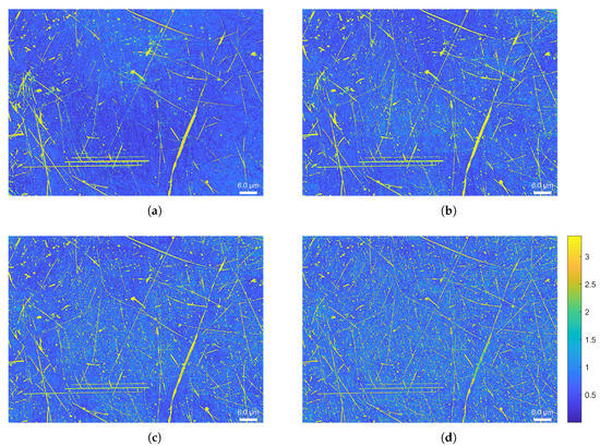
Figure 10.
Scale factor saliency maps estimated with the statistics descriptors calculated from an RTI acquisition of the watch face: (a) Saliency map ; (b) Saliency map ; (c) Saliency map ; (d) Saliency map .
Similar to multi-level saliency, it is possible to calculate multi-scale saliency from several scale factor saliency measurements, as described in Equation (5) and shown in Figure 11.
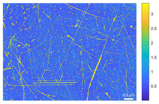
Figure 11.
Multi-scale saliency map estimated with the statistics descriptors calculated from an RTI acquisition of the watch dial. Saliency map multi-scale , , , .
2.4. Synthesis of Multi-Level and Multi-Scale Salience
In Section 2.2, we noted that with multi-level saliency the level of salience of the points decreases when similar points are taken as references. However, by decreasing the size of the sliding window when estimating multi-scale salience, in Section 2.3 we increased the proportionality of the observed and reference salient points when inside the sliding window, thus decreasing the level of salience. We then avoided this drop in the level of salience by coupling the multi-scale method (Equation (4)) to the multi-level method (Equation (3)), as described in Equation (6). It can be observed in Figure 12 that small surfaces anomalies are always visible thanks to the multi-scale approach, while the salience dynamics are increased thanks to the multi-level approach. Thus, the coupling of the two approaches makes it possible to reconcile the discrimination of smaller defects while keeping a large dynamic, which, for example, allows them to be classified and synthetic values of salience to be extracted, thereby integrating the aspects of scale.
where corresponds to the multi-level saliency parameter and and j are the multi-scale saliency parameters.
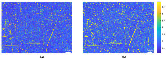
Figure 12.
Multi-level and multi-scale saliency maps estimated with the statistics descriptors calculated from an RTI acquisition of the watch dial: (a) Saliency map multi-scale; (b) Saliency map multi-scale muli-level.
3. Global Approach: Inter-Surface Saliency from RTI Data
The Mahalanobis distance is generally used with the RTI to estimate the visual saliency at each point on the surface. However, the Mahalanobis distance compares observations with a reference sample. Therefore, the observations and reference samples can correspond to other data obtained by the RTI method. In Section 3.1, a method is proposed for estimating distances between several surfaces. This method allows temporal monitoring of the appearance of a surface in order to understand and/or prevent an alteration of the surface state or to explore the surface state manufacturing parameters in order to approach a reference appearance. We then show how this approach can be generalized for analysis of the reconstruction quality of Reflectance Transformation Imaging models in terms of appearance descriptors.
3.1. Distance between Different Surface Roughnesses
In this part, we propose to extend the use of the Mahalanobis distance to both the pixels and to the RTI acquisitions themselves. Thus, we no longer compare the appearance attributes of the points of a surface, only the surface states between them. The comparison of surfaces allows detection of changes in the surface state, helps to observe and prevent anomalies, and enables exploration of the surface state manufacturing parameters in order to approach a reference surface appearance. To compare several surfaces with each other, a distance must be estimated between the local descriptors of the reference surface and the surfaces studied by the Mahalanobis method. When using Equation (1), X then corresponds to the local descriptors of the reference surface and Y corresponds to the local descriptors of the surface for which we want to know the distance. If we have several surfaces to compare with a reference, we obtain several salience maps which discriminate the local changes with an intensity correlated to the degree of change with respect to the reference. Thus, as illustrated in Figure 13, several nickel surfaces can be observed. These surface states have an average roughness () and a maximum roughness (), provided by the manufacturer, that are different for each sample. Then, it can be seen in Figure 14 that the Mahalanobis distance between the surfaces is correlated with the difference of and between the surface reference and the studied surface. To validate these results, an additional study should be conducted to determine the reflectance measurement error and the appropriate normal estimation method [36,37].
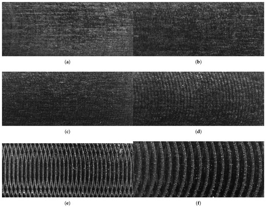
Figure 13.
Raw RTI data of surface state obtained by an end milling process from a surface assembly for roughness control (); ; : (a) Surface R1; ; ; (b) Surface R2; ; ; (c) Surface R3; ; ; (d) Surface R4; ; ; (e) Surface R5; ; ; (f) Surface R6; ; .
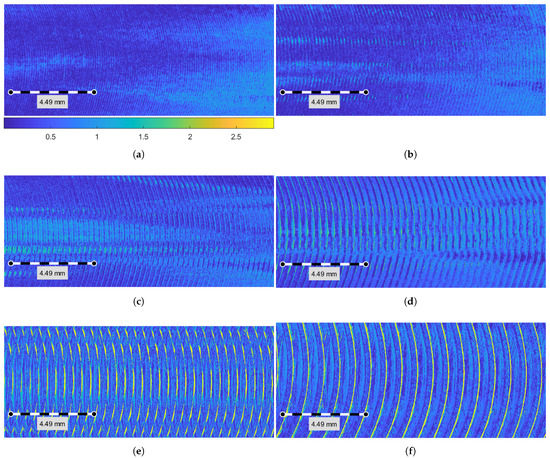
Figure 14.
Mahalanobis distance map calculated with the descriptor of the geometrics descriptors between the surfaces taken from the set : (a) ; (b) ; (c) ; (d) ; (e) ; (f) .
4. Conclusions
A methodology for the evaluation of the visual saliency of surfaces from RTI acquisitions is proposed. This method is based on the implementation of a multi-scale and multi-level approach which integrates the contribution of the local saliency estimated at different scales around the computation point and takes into account the dispersion of the points in the neighborhood for the calculation. The methodology is extended for inter-surface evaluation applications, i.e., for the quantification of the distance in terms of visual properties between different surface roughnesses. The obtained results show that the proposed method can robustly quantify the local appearance properties of the inspected surfaces in the case of local or inter-surface saliency assesment.
Author Contributions
Conceptualization, M.N., G.L.G. and A.M.; Data curation, M.N.; Formal analysis, M.N. and G.L.G.; Funding acquisition, G.L.G.; Investigation, M.N., G.L.G. and P.J.; Methodology, M.N., G.L.G. and A.M.; Project administration, G.L.G. and A.M.; Resources, S.M. and P.J.; Software, M.N.; Supervision, A.M.; Visualization, M.N., G.L.G., P.J. and A.M.; Writing—original draft, M.N.; Writing—review and editing, G.L.G., P.J. and A.M. All authors have read and agreed to the published version of the manuscript.
Funding
This work benefited of the funding of the French National Research Agency (ANR) through the NAPS project (https://anr.fr/Projet-ANR-17-CE10-0005).
Institutional Review Board Statement
Not applicable.
Informed Consent Statement
Not applicable.
Data Availability Statement
Not applicable.
Conflicts of Interest
The authors declare no conflict of interest. The funders had no role in the design of the study; in the collection, analyses, or interpretation of data; in the writing of the manuscript, or in the decision to publish the results.
References
- Brown, C.A.; Hansen, H.N.; Jiang, X.J.; Blateyron, F.; Berglund, J.; Senin, N.; Bartkowiak, T.; Dixon, B.; Goic, G.L.; Quinsat, Y. Multiscale analyses and characterizations of surface topographies. CIRP Ann. 2018, 67, 839–862. [Google Scholar] [CrossRef]
- Lemesle, J.; Goic, G.L.; Mansouri, A.; Brown, C.A.; Bigerelle, M. Wear Topography and Toughness of Ceramics correlated in Metal Matrix Composites using Curvatures by Reflectance and Multiscale by Filtering. In Proceedings of the 22nd International Conference on Metrology and Properties of Surfaces, Lyon, France, 3–5 July 2019. [Google Scholar]
- Berglund, J.; Brown, C.A.; Rosèn, B.G.; Bay, N. Milled Die Steel Surface Roughness Correlation with Steel Sheet Friction. CIRP-Ann.-Manuf. Technol. 2010, 59/1, 577–580. [Google Scholar] [CrossRef]
- Le Goic, G.; Benali, A.; Nurit, M.; Cellard, C.; Sohier, L.; Mansouri, A.; Moretti, A.; Créa’hcadec, R. Reflectance Transformation Imaging for the quantitative characterization of Experimental Fracture Surfaces of bonded assemblies. Eng. Fail. Anal. 2022, 140, 106582. [Google Scholar] [CrossRef]
- Belaud, V.; Valette, S.; Stremsdoerfer, G.; Bigerelle, M.; Benayoun, S. Wettability versus roughness: Multi-scales approach. Tribol. Int. 2015, 82, 343–349. [Google Scholar] [CrossRef]
- Luxman, R.; Castro, Y.E.; Chatoux, H.; Nurit, M.; Siatou, A.; Le Goïc, G.; Brambilla, L.; Degrigny, C.; Marzani, F.; Mansouri, A. LightBot: A Multi-Light Position Robotic Acquisition System for Adaptive Capturing of Cultural Heritage Surfaces. J. Imaging 2022, 8, 134. [Google Scholar] [CrossRef] [PubMed]
- Zendagui, A.; Goïc, G.L.; Chatoux, H.; Thomas, J.B.; Jochum, P.; Maniglier, S.; Mansouri, A. Reflectance Transformation Imaging as a Tool for Computer-Aided Visual Inspection. Appl. Sci. 2022, 12, 6610. [Google Scholar] [CrossRef]
- Malzbender, T.; Gelb, D.; Wolters, H. Polynomial texture maps. In Proceedings of the SIGGRAPH’01, Computer Graphics and Interactive Techniques, Los Angeles, CA, USA, 12–17 August 2001; pp. 519–528. [Google Scholar]
- Jung, S.; Woo, S.; Kwon, K. Apparatus and Method of Reading Texture Data for Texture. Mapping. Patent US8605101B2, 10 December 2013. [Google Scholar]
- Gautron, P.; Krivanek, J.; Pattanaik, S.; Bouatouch, K. A Novel Hemispherical Basis for Accurate and Efficient Rendering. In Proceedings of the ESGR’04 Papers, Eurographics Conference on Rendering Techniques, Norköping, Sweden, 21–23 June 2004 2004; pp. 321–330. [Google Scholar]
- Ciortan, I.M.; Pintus, R.; Marchioro, G.; Daffara, C.; Giachetti, A.; Gobbetti, E. A Practical Reflectance Transformation Imaging Pipeline for Surface Characterization in Cultural Heritage. In Proceedings of the Eurographics Workshop on Graphics and Cultural Heritage, Genova, Italy, 5–7 October 2016; Catalano, C.E., Luca, L.D., Eds.; The Eurographics Association: Reims, France, 2016. [Google Scholar]
- Pitard, G.; Le Goic, G.; Favreliere, H.; Samper, S. Discrete Modal Decomposition for surface appearance modelling and rendering. In Proceedings of the SPIE 9525, Optical Measurement Systems for Industrial Inspection IX, Munich, Germany, 22–25 June 2015; p. 952523. [Google Scholar]
- Pintus, R.; Dulecha, T.; Jaspe, A.; Giachetti, A. Objective and Subjective Evaluation of Virtual Relighting from Reflectance Transformation Imaging Data. In Proceedings of the EG GCH, Eurographics Workshop on Graphics and Cultural Heritage, Vienna, Austria, 11–15 November 2018. [Google Scholar]
- Le Goïc, G. Qualité géoméTrique & Aspect des Surfaces: Approches Locales et Globales. Ph.D. Thesis, Université de Grenoble, Grenoble, France, 2012. [Google Scholar]
- Pitard, G.; Le Goic, G.; Mansouri, A.; Favreliere, H. Discrete Modal Decomposition: A new approach for the reflectance modeling and rendering of real surfaces. Mach. Vis. Appl. 2017, 28, 607–621. [Google Scholar] [CrossRef]
- Pitard, G.; Le Goic, G.; Mansouri, A.; Favreliere, H. Robust Anomaly Detection Using Reflectance Transformation Imaging for Surface Quality Inspection. In Proceedings of the SCIA, Scandinavian Conference on Image Analysis, Tromsø, Norway, 12–14 June 2017; Volume 10269, pp. 550–561. [Google Scholar]
- Lemesle, J.; Robache, F.; Le Goïc, G.; Mansouri, A.; Brown, C.; Bigerelle, M. Surface Reflectance: An Optical Method for Multiscale Curvature Characterization of Wear on Ceramic–Metal Composites. Materials 2020, 13, 1024. [Google Scholar] [CrossRef] [PubMed]
- Giachetti, A.; Ciortan, I.; Daffara, C.; Pintus, R. Multispectral RTI Analysis of Heterogeneous Artworks. In Proceedings of the EG GCH, Eurographics Workshop on Graphics and Cultural Heritage, Graz, Austria, 27–29 September 2017. [Google Scholar]
- Ponchio, F.; Corsini, M.; Scopigno, R. Relight: A compact and accurate RTI representation for the Web. Graph. Model. 2019, 105, 101040. [Google Scholar] [CrossRef]
- Castro, Y.; Nurit, M.; Pitard, G.; Zendagui, A. Calibration of spatial distribution of light sources in reflectance transformation imaging based on adaptive local density estimation. J. Electron. Imaging 2020, 29, 1–18. [Google Scholar] [CrossRef]
- Dulecha, T.G.; Pintus, R.; Gobbetti, E.; Giachetti, A. SynthPS: A Benchmark for Evaluation of Photometric Stereo Algorithms for Cultural Heritage Applications. In Proceedings of the EG GCH, Eurographics Workshop on Graphics and Cultural Heritage, Online, 18–19 November 2020. [Google Scholar]
- Florindi, S.; Revedin, A.; Aranguren, B.; Palleschi, V. Application of Reflectance Transformation Imaging to Experimental Archaeology Studies. Heritage 2020, 3, 1279–1286. [Google Scholar] [CrossRef]
- Iglesias, C.; Martínez, J.; Taboada, J. Automated vision system for quality inspection of slate slabs. Comput. Ind. 2018, 99, 119–129. [Google Scholar] [CrossRef]
- Smith, M.; Stamp, R. Automated inspection of textured ceramic tiles. Comput. Ind. 2000, 43, 73–82. [Google Scholar] [CrossRef]
- Martlin, B.; Rando, C. An assessment of the reliability of cut surface characteristics to distinguish between hand-powered reciprocating saw blades in cases of experimental dismemberment. J. Forensic Sci. 2020, 66, 444–455. [Google Scholar] [CrossRef] [PubMed]
- Coules, H.; Orrock, P.; Seow, C. Reflectance Transformation Imaging as a tool for engineering failure analysis. Eng. Fail. Anal. 2019, 105, 1006–1017. [Google Scholar] [CrossRef]
- Le Goic, G. Geometric Quality and Appearance of Surfaces: Local and Global Approach. Ph.D. Thesis, University of Savoie Mont-Blanc, Chambéry, France, 2012. [Google Scholar]
- Baudet, N.; Pillet, M.; Maire, J.L. Visual inspection of products: A comparison of the methods used to evaluate surface anomalies. Int. J. Metrol. Qual. Eng. 2011, 2, 31–38. [Google Scholar] [CrossRef][Green Version]
- Guerra, A.S. Métrologie Sensorielle Dans le Cadre du Contrôle Qualité Visuel. Ph.D. Thesis, Université de Savoie, Chambéry, France, 2008. [Google Scholar]
- Debrosse, T.; Pillet, M.; Maire, J.L.; Baudet, N. Sensory perception of surfaces quality—Industrial practices and prospects. In Proceedings of the Keer 2010-International Conference on Kansei Engineering and Emotion Research, Paris, France, 2–4 March 2010. [Google Scholar]
- Pitard, G. Métrologie et Modélisation de l’Aspect pour l’Inspection qualité des Surfaces. Ph.D. Thesis, Université Grenoble Alpes, Grenoble, France, 2016. [Google Scholar]
- Kim, Y.H.; Choi, J.; Lee, Y.Y.; Ahmed, B.; Lee, K.H. Reflectance Transformation Imaging Method for Large-Scale Objects. In Proceedings of the 2016 13th International Conference on Computer Graphics, Imaging and Visualization (CGiV), Beni Mellal, Morocco, 29 March–1 April 2016; pp. 84–87. [Google Scholar]
- Nurit, M.; Le Goïc, G.; Lewis, D.; Castro, Y.; Zendagui, A.; Chatoux, H.; Favrelière, H.; Maniglier, S.; Jochum, P.; Mansouri, A. HD-RTI: An adaptive multi-light imaging approach for the quality assessment of manufactured surfaces. Comput. Ind. 2021, 132, 103500. [Google Scholar] [CrossRef]
- Mahalanobis, P.C. On the Generalized Distance in Statistics; National Institute of Sciences: Calcutta, India, 1936; Volume 2, pp. 49–55. [Google Scholar]
- Nouri, A.; Charrier, C.; Lézoray, O. Multi-scale mesh saliency with local adaptive patches for viewpoint selection. Signal Process. Image Commun. 2015, 38, 151–166. [Google Scholar] [CrossRef]
- Obein, G. Métrologie de l’Apparence; Hdr, CNAM: Paris, France, 2018. [Google Scholar]
- Quéau, Y.; Durou, J.; Aujol, J. Variational Methods for Normal Integration. arXiv 2017, arXiv:1709.05965. [Google Scholar] [CrossRef]
Publisher’s Note: MDPI stays neutral with regard to jurisdictional claims in published maps and institutional affiliations. |
© 2022 by the authors. Licensee MDPI, Basel, Switzerland. This article is an open access article distributed under the terms and conditions of the Creative Commons Attribution (CC BY) license (https://creativecommons.org/licenses/by/4.0/).