1. Introduction
During the last couple of years, the coronavirus pandemic has put healthcare systems from all around the globe under extreme stress. Most hospitals have seen their infrastructure and capacity to offer quality health care collapsing under an unexpected and enormous demand, and despite COVID-19 having obviously been the main actor in this crisis, the whole situation has evidenced some big inefficiencies of the system.
The healthcare service delivered in hospitals depends, to a large extent, on the efficiency in the execution of all those medical and non-medical processes aimed at providing, altogether, quality service to the patient. Busy healthcare systems continue to challenge their managers and decision-makers due to high demands, high costs, limited budgets, and health resources. As a result, decision-makers are constantly examining the efficiency of existing healthcare systems and must be able to evaluate the outcomes of any changes they make to those systems [
1]. These activities and relationships are often complex and multidisciplinary, making them a major focus of study as not only the development and application of advanced analytical methods but also their optimization. Both of these can result in improvements in many different areas simultaneously, such as the reduction in administrative costs [
2], the optimization of hospital resources [
1], and the reduction in patient waiting times or a greater degree of service customization [
3]. This results in a higher quality service that is appreciated by both institutions and users alike.
The emergency department (ED) is the service with the highest demand in a hospital, and this is continuously increasing, reaching a critical point. The number of patients visiting the ED has been steadily rising worldwide for the last few decades, which has led to situations of overcrowding in emergency rooms all around the globe. Data from the Institute of Medicine in the United States already identified crowding as a critical threat to the quality of the service provided to patients back in 2006 [
4]. Similarly, the Spanish Ministry of Health released data regarding ED usage in 2010 which showed an increase of 23.2% in ED visits between 2001 and 2007 [
5], with an ED usage frequency rate notoriously higher than that of the UK or the US. The latest report showed a 9% increase in the number of visits attended in hospitals in Spain between 2014 and 2018, without any specific health reasons or population growth to account for that change.
ED crowding has been described by the American College of Emergency Physicians (ACEP) [
6] as “a situation in which the need for emergency services outstrips available resources in the ED. This situation occurs in hospital EDs when there are more patients than staffed ED treatment beds and wait times exceed a reasonable period.”
A health emergency, on the other hand, has been defined by the WHO as the unexpected appearance of a health issue of any type and cause, of varying degrees of seriousness, that generates an imminent need for attention or treatment by a professional. Therefore, EDs need to offer a multidisciplinary assistance service, complying with functional, structural, and organizational requisites to guarantee safety, quality, and efficient conditions to attend to any possible emergency.
Despite this, crowding hinders the ability of EDs around the world to deliver such a service in optimal conditions. Existing studies show the direct correlation of ED crowding with increased ED waiting times, decreased patient satisfaction, inadequately treated pain, higher walkaway rates, and even higher mortality [
7,
8,
9,
10]. Furthermore, hospital staff suffer from the consequences of overcrowding, showing dissatisfaction, frustration, and stress, and facing higher exposure to violence and physical aggression [
11]. The optimization of this service and all the processes behind it must therefore be a priority in order to guarantee the continuity and improvement of its quality.
Reasons for the increase in this phenomenon are varied as illustrated in
Table 1. It has been observed by experts that patients are increasingly demanding immediate health checks for non-urgent conditions. However, some experts also identify problems in the structure, which is not always able to solve problems quickly enough in the primary attention system, which is marked by long waiting times and is therefore being abandoned by users.
One of the processes that has the greatest impact on emergency room congestion is the admission of patients from the ED into the hospital, as a result of the required logistics for patient management and bed allocation. The impact of an inefficient patient admission process in the ED is of high relevance. While only around 11% of the visits to the ED department end in an admission to the hospital, EDs are still the largest source of hospital admissions. Lengthy boarding times of patients that are waiting to be assigned a bed at the hospital use precious resources such as time, space, and medical attention, which should instead be used in other ED tasks, and contribute to the overcrowding of the service [
12].
Over the past few years, various solutions have been proposed to resolve this issue, the most significant of which is the simplification of the admission procedure [
13], the addition of more doctors to the admission process of both hospitals and emergency department [
3,
14,
15], an optimized process of early hospital discharges [
16,
17], or the creation of an ED dependent unit for short-length stays [
18]. However, none of them appears to be easily implementable without significant economic investment, or sustainable in a situation in which the number of visits to emergency departments will continue to rise.
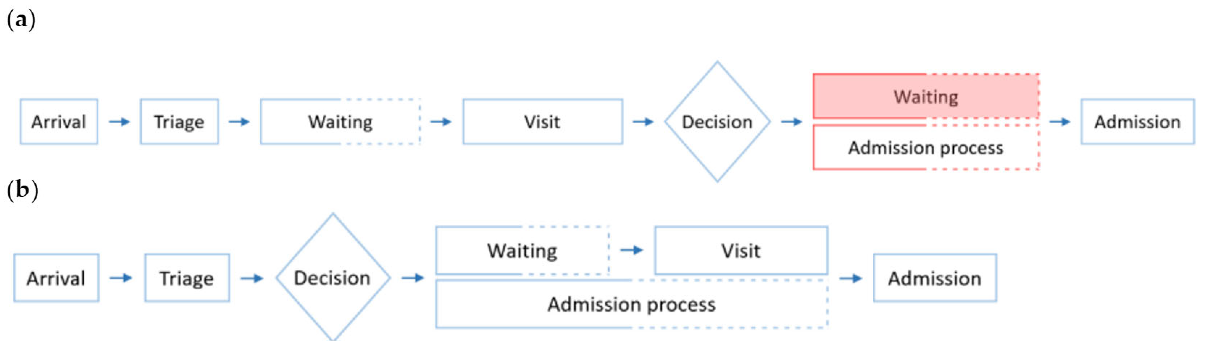
In contrast, monitorization of the admission process and anticipation of hospital admissions can potentially help optimize the use and allocation of resources in a sustainable way, thus improving the quality of emergency care and user satisfaction. Data collected in hospital databases and shared through Health Information Exchange (HIE) platforms can be used to make early predictions of inpatient admission and assist the implementation of actionable measures. In the current system, the process of inpatient admission to the hospital from the ED starts after the visit is completed. That means that after the visit, the patient must wait in ED facilities—crowding them unnecessarily—while the administrative staff processes their admission and allocates them a bed in the hospital. With an early prediction of admission, for example at the moment of arrival of the patient in the ED, the administrative staff would be able to carry out this process while the patient goes through the ED visit in a simultaneous rather than sequential way. By doing so, if the patient had to be indeed admitted into the hospital after the visit, the admission process would have already been completed and there would be no extra waiting time nor unnecessary crowding, as portrayed in
Figure 1.
In spite of some studies [
3,
13,
19] showing that patient visit data can improve the predictive performance slightly when compared with a model predicting admissions at the time of arrival, this study aims at predicting admissions using information readily available at the moment of triage, immediately following the arrival of the patient at the ED by analyzing data from more than 60 different centers in the Integral Healthcare System for Public Use in Catalonia (SISCAT). Triage is the first stage of an ED visit and its objective is to assess in a regulated, validated, and reproducible way, and as accurately as possible, the level of urgency of a visit to organize patients in recognizable groups to prioritize the sickest ones [
20]. The primary reason for performing this is that the sooner admissions are initiated, the higher the chance of being able to reduce ED crowding, which is the ultimate objective of developing a predictive model for hospital admissions. Moreover, the predictive models might help reduce overcrowding at EDs and improve the service delivered to patients. The first step of this paper was to identify data requirements followed by pre-processing data. Then, a gradient boosting machine was used to train and test the predictive models in R. After that, variable importance for each of the models was analyzed, receiver operating characteristic (ROC) curves were created, and the area under the curve (AUC) was obtained from each of them as a measure of predictive performance. Finally, the results were obtained and future works were proposed.
2. Literature Review
Prediction models in healthcare seek to increase logistical efficiency, enhance resource allocation, reduce patient waiting time, and improve patient care. During the last fifteen years, researchers have put attention to data collected early in ED encounters to help existing triage systems more quickly to identify and prioritize patients with critical conditions from the volumes of those with less urgent needs to tackle and possibly alleviate ED overcrowding.
Triage is usually performed by a member of the nursing staff based on the patient’s demographics, chief complaint, and vital signs. The patient is then seen by a healthcare provider, who develops the initial plan of care and ultimately recommends triage [
21]. There are many different triage systems. Among them, the most widely accepted is the Australian Triage Scale (ATS) [
22], the Canadian Triage Acuity Scale (CTAS) [
23], and the Manchester Triage System (MTS) [
24]. However, there are other approved systems such as the Andorran Triage Model (MAT) [
25], which is used in almost all the hospitals in the Catalan healthcare system.
Researchers have been implementing machine learning algorithms, in different forms, to extract valuable information from the huge amounts of data existing in hospital and ED databases. These algorithms are capable of understanding patterns in data and building corresponding models that use the identified patterns to classify new observations. Some basic studies have been researched on the topic with the development of models to predict future ED visits, thus facilitating the provision and preparation of ED staff to avoid overcrowding. Penades and Ros (2015) used ARIMA and Holt–Winters models to demonstrate that such predictions were possible with mean errors of 2.5% and 3.84%, respectively, when predicting visits at a monthly level [
26].
More complex models have attempted to predict, not the number of visits, but the percentage of these that will turn into an admission to the hospital. The first studies were centered in trauma level I centers, in which the reasons for visiting are not as varied as in a general hospital ED, and the severity of disease (or injury in this case) can be more objectively assessed at triage. Probabilistic systems in the form of a Bayesian network for early prediction of admission in ED in these centers, with data available early in the ED visit, proved to be useful for predicting patient admissions already in 2005 (AUC = 0.894) [
19]. (The specificity in these models is to be understood as the capacity of the algorithm to correctly predict the discharges, i.e., a specificity of 90% means 90 out of 100 discharges were predicted as such with the model, while 10 out of 100 were wrongly predicted as admissions). The same researchers concluded in 2006 that artificial neural networks (ANN) could also be used to predict hospital admissions in pediatric ED encounters, again in trauma level I centers, showing an almost equal performance (AUC = 0.897) [
27].
More recently, logistic regression and Naive Bayes analysis have been used extensively to make predictions in the healthcare field. Savage et. al. (2017) applied logistic models on triage administrative data to estimate admissions to the ED (AUC = 0.78), which in turn is used to predict the number of hours of bed requirements for the ED. The logistic regression models obtained had a sensitivity of 23% and a specificity of 97%. Even though these results were satisfactory for particular admission predictions, the hourly pooled probabilities of bed requirements showed better results, which are consistent with historical demand [
28].
Barak-Corren, Fine, & Reis (2017) [
12] have investigated to improve accuracy (percentage of predictions, of both admissions and discharges, that conform to the real observed value) on the combination of different analytical tools with the logistic regression approach. Applying a logistic regression model on results generated by a Naive Bayes classifier from data collected within the first 30 min from arrival yielded good results in their study, identifying more than 73% of admissions with a 90% specificity and over 35% with 99.5% specificity, or what is the same, a false-positive rate of 0.5% (AUC = 0.91). The method has also been applied to predict admissions at the moment of arrival (after 0 min), successfully identifying 50.6% of the hospitalizations with a 10% false-positive rate and obtaining an overall AUC = 0.79 [
12].
Other researchers have explored manipulating the data slightly to obtain models that would show better performance measures and higher accuracy. Lucke et al. (2018) [
29]
https://orcid.org/0000-0003-0617-8873 showed that it was possible to increase the prediction accuracy of admission at the time of arrival for patients visiting the ED with a logistic regression model by dividing the observations into two groups, one containing those related to patients under 70 years old (AUC = 0.86), and a second one including the rest, i.e., those containing observations of patients above 70 years old (AUC = 0.77) [
29].
The random forest technique has also been used in this field to develop an e-triage model to predict the likelihood of acute outcomes that may lead to admission. Levin et al. (2018) obtained models with AUC ranging from 0.73 to 0.92 for different datasets [
30]. Although the objective of their study was more focused on the demonstration that the current triage systems could be improved through the use of information extracted from patient data upon arrival at the ED, it also showed the potential of these models to predict hospital admission with significant accuracy.
Furthermore, a study from 2018 [
21] set the objective to determine which, among the most popular predictive techniques, could provide the best performance. Training models on triage information yielded a test AUC of 0.87 for all logistic regression, gradient boosting, and deep neural networks (DNN) models. However, the study went further on to prove that combining triage information with patient history could significantly improve predictive performance for all three methods, achieving an AUC of 0.91 for the logistic regression model, and 0.92 for the gradient boosting and the DNN models. Models trained on patient history information exclusively did not yield better results than those trained with triage data alone. They also explored that the gradient boost and DNN outperformed logistic regression on the full dataset while there was no significant difference in performance between them [
21].
3. Method and Materials
3.1. Study Setting
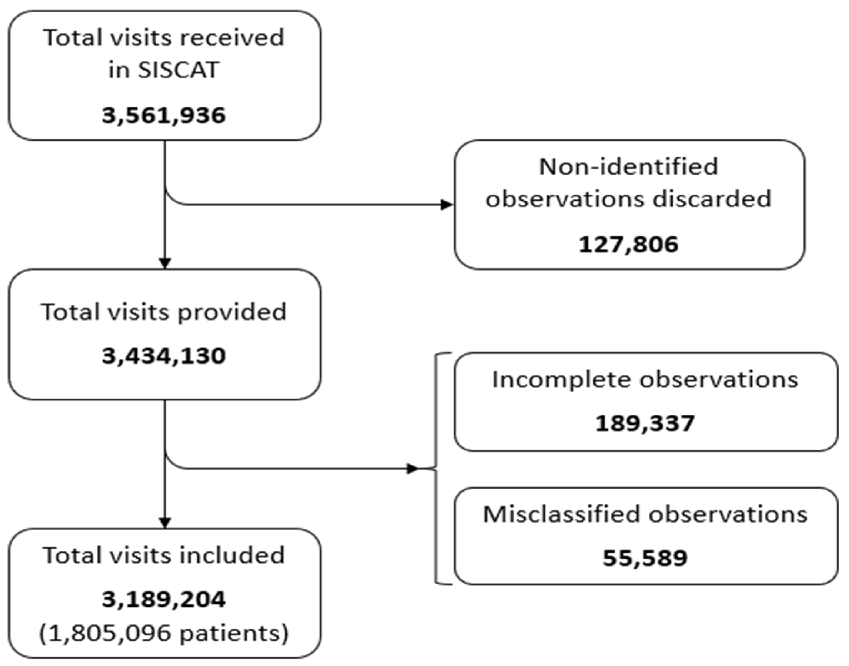
A retrospective analysis of all visits to EDs of hospitals included in the Integral Healthcare System for Public Use in Catalonia from 1 January 2018 to 31 December 2018, containing 3,189,204 observations (after pre-processing stage), was conducted.
The data were provided by the Catalan Government through the Catalan Healthcare System (Servei Català de Salut, CatSalut) including all the observations that had been correctly identified with the anonymized patient ID. In this pre-processing stage carried out by the governmental entity, 127,806 observations were left out due to missing or erroneous identification numbers (ID), accounting for 3.6% of the total emergency visits. The remaining observations, correctly identified, recorded disposition of either admission or discharge after the visit to the ED. The data were provided in .dat format, which could be directly imported to RStudio for processing.
3.2. Feature Extraction
For each observation, the following fields were included: identifier, age, gender, main diagnosis of the urgency based on the Clinical Classification System (CCS) system, triage level according to the MAT system, and admission result in binary format. Age information was either obtained at triage or available from the Electronic Health Records; for patients under 1 year of age, an extra variable containing the age in days was included. Different visits with the same identifier were classified as different observations.
3.3. Data Preparation
Some variables were either added or modified to increase predictive performance of the model. First, the dataset was cleansed to eliminate all those observations that were incomplete, which accounted for 189,337 observations (5.51%). Following this first cleansing, a quick analysis was performed to identify variables that might have abnormal values; 34,725 (1.01%) observations were eliminated for containing non-existent triage values, i.e., >5. In the category of symptoms (CCS), some observations had been classified as “incomplete” and were eliminated from the dataset as well; that accounted for 20,864 observations and 0.61% of the initial total.
After this pre-processing stage of the data performed by both the government and the researcher, the number of observations for analysis dropped from 3,561,936 to 3,189,204. (See
Figure 2).
An extra variable was created to show the accumulated number of visits for each patient during the year observing that it was recurrent to have multiple visits for one patient in the 2018 exercise. The same procedure was used to see the absolute frequencies for the symptoms (CCS) variable, and a feature selection procedure was conducted to reduce the number of levels with very little frequency. In this case, it was decided to assign the label “Other” to all these observations whose CCS value appeared fewer than 30 times throughout the dataset. This would imply an average of less than one case every ten days in the whole Integral Healthcare System for Public Use in Catalonia, on average.
Table 2 shows the number of distinct outcomes observed for each of the variables in the dataset.
Some of these variables were classified as numerical by default although they were categorical. Prior to analyzing the data, gender, CCS, and triage were factored. Lucke, J.A. et al. (2018) [
29] state that accuracy of the prediction at time of arrival for patients visiting the ED could be improved by dividing the observations into two subsets, (1) containing all those related to patients under 70 years of age; and (2) containing all those above 70, a division of the main dataset. To further contrast this enhanced predictive value, another division was created with the 18 years of age threshold in order to test the performance of a model dedicated to pediatrics against that of a model for adults. This resulted in 5 distinct datasets: the complete dataset, the pediatrics dataset [0–18] years, the adults dataset [18, 115] years, the adults under 70 dataset [18, 70] years (i.e., young adults dataset), and the adults over 70 dataset [70, 115] years (i.e., old adults dataset). For all the datasets, the variable age days was eliminated.
3.4. Gradient Boosting
Gradient boosting is a machine learning algorithm that builds an ensemble of weak trees in a sequential fashion, with each tree being trained with respect to the previous and reducing the marginal error of the whole ensemble learned so far [
31]. Subsequent trees, therefore, help classify observations that are not well classified. Later, weak trees are combined in a gradual and additive manner into a powerful and strong model with high predictability, which is hard to beat with other algorithms [
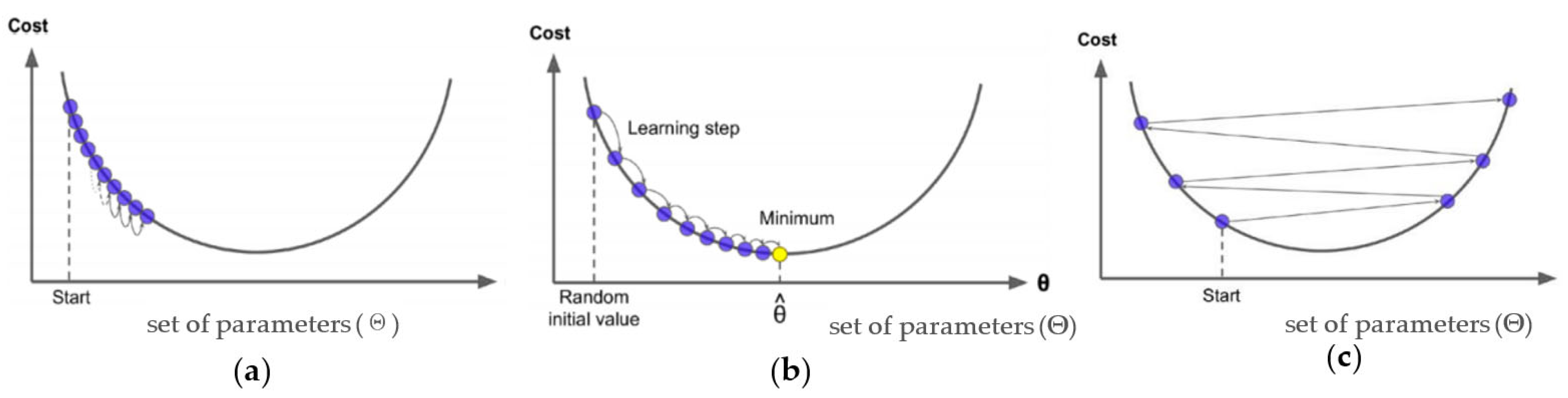
32]. The theory behind this process is to train the new base learners to be maximally correlated with the negative gradient of the loss function associated with the whole ensemble until the gradient descent is zero. In other words, the gradient descent measures the local gradient of the loss (cost) function for a given set of parameters (Θ) as illustrated in
Figure 3.
For datasets with a categorical response 𝑦 ∈ {0, 1}, the two most used loss functions are the Binomial and the Adaboost loss function, which are more generally referred to as the Bernoulli loss functions. Given that gradient boosting machines (GBM) learn sequentially from previous weak models, it is of high relevance to defining an adequate shrinkage value. This value can help regularize and control model complexity by potentially reducing the impact of unstable regression coefficients and reducing the size of incremental steps in the model learning process. The main principle applied is that taking many small steps in improving the model is better than taking fewer large steps. The shrinkage parameter is defined as 𝜆 ∈ (0, 1] [
33]. Although the number of weak trees to train is defined by the researcher, for small values of 𝜆 the gradient boosting algorithm will require many trees (>1000) to arrive at a satisfactory result (see
Figure 3), which can be computationally expensive and time-consuming.
In spite of this, reducing shrinkage too much can result in a negative outcome, known as overfitting. This is defined as an excessive improvement of the model to the training dataset, learning and adapting too much on its particularities and resulting in a decrease in the performance on the test dataset. This can be solved with the early stopping technique, which allows the algorithm to stop the number of iterations before the initially pre-specified one if it detects overfitting, or what is the same, a decrease in the predicting power of observations in the test set. This optimal number of boosts is therefore dependent on the shrinking parameter λ. To deal with the trade-off existing between the learning rate and number of boosts is usually approached using a cross-validation procedure, which allows for testing the model on withheld portions of data, while still using all of the data at the processing stages. To do so, a cross-validating parameter k is defined and used to partition the data into k disjoint non-overlapping subsets, each of which will be used as a validation set for the GBM model fitted with the rest of the subsets. Only after doing the process for all the subsets will the validation performance from each of the folds be aggregated to serve as estimate of model generalization on the validation set [
31].
One of the disadvantages of gradient boosting machines, apart from overfitting, is the comparably low interpretability of the results obtained. There are two main tools to address this issue. The first one is the relative variable influence analysis [
34], which is a common tool used in many cases to base the feature selection, although it does not provide any specific explanation of how each variable actually affects variation in the result. The second tool is partial dependence plots, which are commonly used to visualize the effect of one selected variable on the response while controlling for the effect of all other explanatory variables. These graphs may be less insightful when interactions between variables have significant impact on results, but they have been proven to provide a solid basis for interpretation of the models [
35].
The most valuable feature of GBMs is that they are highly flexible. As mentioned, parameters such as number of trees, depth of trees, learning rate, and subsampling can be modified to tune the training model and improve its efficiency while enhancing overall performance [
36]. In other words, GBM is a powerful tool for predictive modeling, and one of the best algorithms in classification tasks, providing higher accuracy and better results than other conventional single strong models and better predictive performance than logistic regression [
17,
34], no studies had used it before with the objective of predicting hospital admissions in EDs at the moment of triage.
3.5. Model Fitting and Validation
The models were trained on each of the five datasets described above using gradient boosting machine in R, using the “gbm”, “caret”, “ROCR” and “pROC” packages. Each of these datasets was divided into training sets and test sets, randomly sorting 70% of the observations to the former and the remaining 30% to the latter. The training set was used to build the model for the gradient boosting machine, analyze the variable importance in predicting the outcome, and test for overfitting. The test set was used to evaluate the predictive performance of the model trained with a confusion matrix from which to extract the performance parameters (accuracy, sensitivity, specificity, positive predictive value (PPV), and negative predictive value (NPV)) and create the receiver operating characteristic (ROC) curve, therefore obtaining the AUC for each of the models, with a 95% confidence interval obtained with the DeLong method [
37].
The gradient boosting models were developed with a Bernoulli distribution function since it was considered the best option to predict the binary response [
38]. A total of 1000 trees were used to train all the models, with an interaction depth of 3 levels and a shrinkage equal to 0.01. To ensure that the trained models were not overfitted, a tuning process was performed for all of them using the exact same parameters and adding 2-fold cross-validation.
Variable importance is an indicator of the information gain that a given variable provides in a split. The rank for variable importance was obtained for each of the models and used to create models including only the three most influential variables checking whether it was possible to obtain the same levels of predictive performance.
Predictions for the accuracy testing were completed using 1000 trees as well and setting a threshold for prediction to 0.5; that is, if a prediction yielded a result with more than 50% probability of being an admission, it would be classified as an admission. Confusion matrixes were obtained from the predicted results. Information about performance was also obtained from the receiver operating characteristic curve for each model, where the true positive rate was plotted against the false positive rate. Moreover, these curves allowed for the obtention of the area under the curve, which was provided with a 95% confidence interval following the method described by DeLong [
37].
With the same models used for the first part of the research, which targeted high-accuracy results, the second part of the study was approached. In this sense, the objective was to obtain high sensitivity levels (>0.975) while maintaining a specificity over 0.33. This was achieved by lowering the probability of admission required to classify an observation as such, and changing the range from 0.05 to 0.01 in order to predict as many admissions as possible.
This procedure was conducted for each of the models until the required sensitivity level was obtained, and the specificity level was checked after reaching the critical point. These models presented a trade-off between the ability to detect 97.5% of all the observed admissions, and the ability to correctly predict as many outcomes as possible. As will be discussed below, targeting high sensitivity levels made the number of false positives increase substantially. These models would therefore not be adequate for implementation in the ED, for the staff would anticipate more admissions than really observed, and a lot of resources would be wasted in preparing for these false positives. However, these models can have a very high potential for implementation, not for hospital use but for patient use, to allow for the first contact between patient and ED, and regulate the number of patients self-referring to the ED for non-urgent causes. A more in-depth explanation has been developed in the discussion.
4. Results
4.1. Sample Characteristics
During the year 2018, the EDs in the Integral Healthcare System for Public Use in Catalonia received a total of 3,561,936 individual visits, 3,434,130 of which were included in the dataset provided by the Catalan Healthcare System to perform the study. After cleansing the data, 3,189,204 observations that had been correctly identified and classified were included. These accounted for 1,805,096 unique patients.
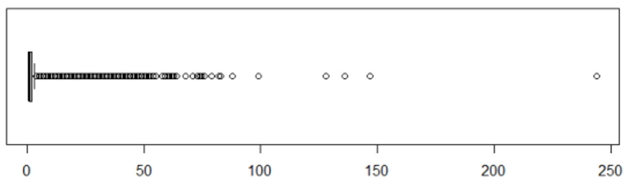
The accumulated number of visits per patient ranged from 1 to 244, with a median of 1, and a mean equal to 1.767. A box plot of the absolute frequencies of visits per patient can be found in
Figure 4, in which the outlier values regarding the number of visits are clearly visible.
The overall admission rate was 11.018%, with 351,391 admissions by 275,875 unique patients, and 2,837,813 discharges by 1,690,092 different patients.
Looking for an indicator of admission in the frequency of visits, a correlation analysis was performed using the Pearson correlation method. This yielded a result of 0.01, an extremely weak correlation indicating that both variables are hardly related. Further, a
p-value < 0.001 was obtained, giving undeniable significance to the test result. To observe the behavior of these two variables against each other,
Figure 5 is presented.
The gender distribution of the sample was 46.44% male and 53.56% female, with a rate of admission slightly higher for the former, 11.41% against 10.68%, which proved to be statistically significant with alpha equal to 0.001 (
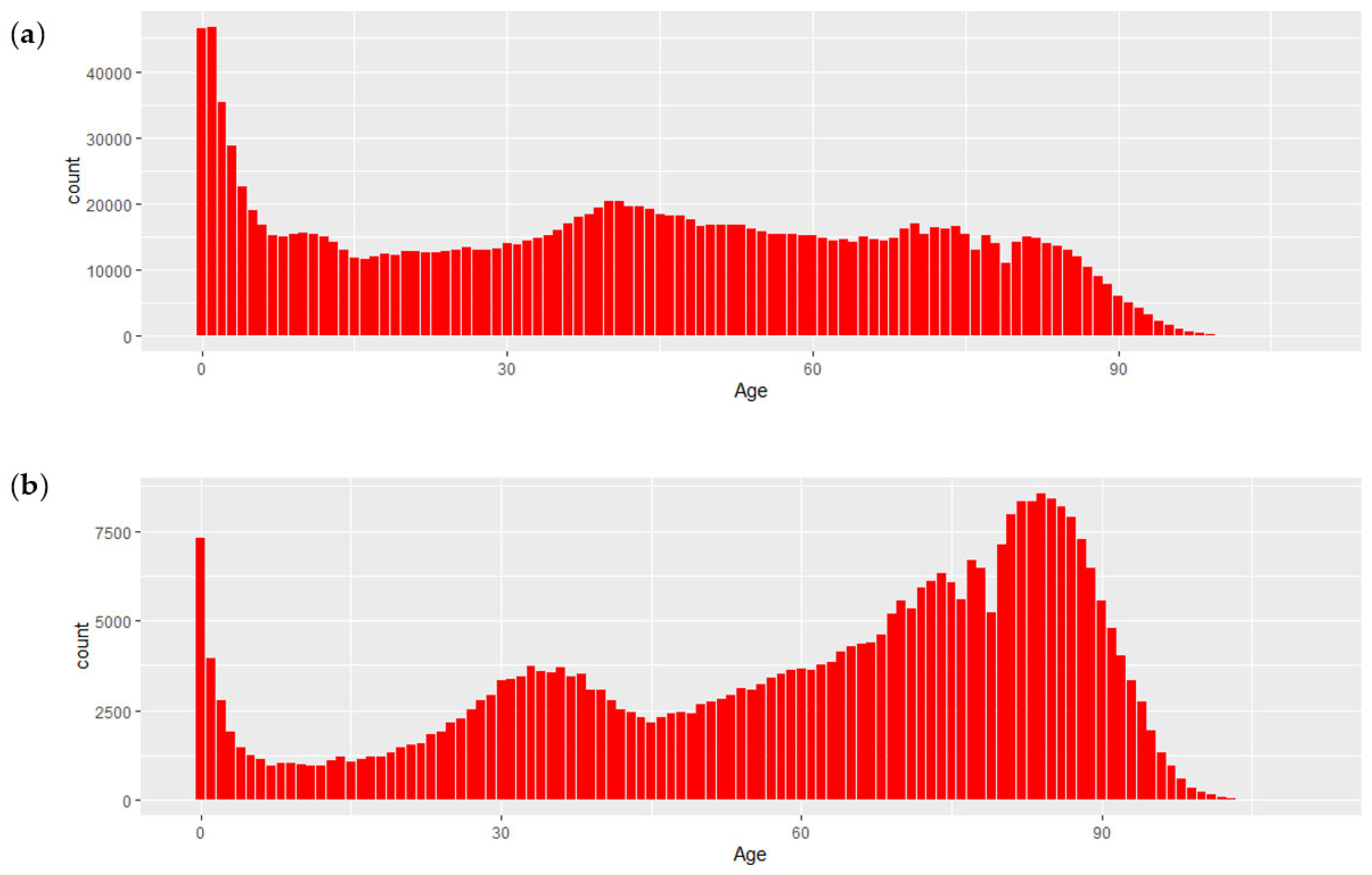
p-value < 0.001). The average age of the patients included in the study was 43.08 years old, slightly higher for females (44.90), than for males (41.91). Charts for the gender-specific age distribution can be found in
Figure 6. The average age for those visits that ended in an admission to the hospital was 59.57 years old, while that of those visits that ended in discharge was 41.04 years old, a more than 18 points difference that was clearly significant with a
p-value < 0.001 for alpha equal to 0.001.
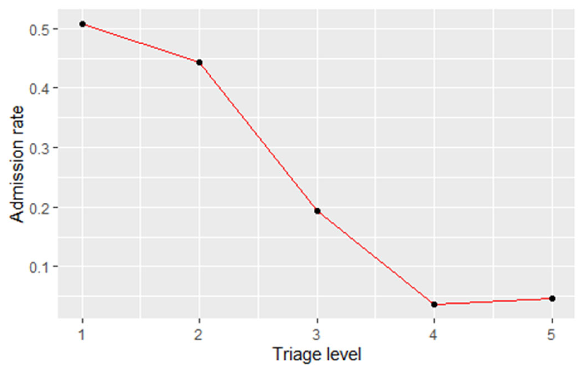
Regarding the triage level frequencies, it is concluded that one accounts for the most urgent and priority cases and five for the least urgent ones. Moreover, it is worth noticing the statistically significant higher severity (p-value < 0.001, alpha = 0.001) of the classification of patients admitted in front of patients discharged; the former had an average triage level of 3.03, while the latter had a 3.74 average triage level.
Figure 7 shows the admission rates for all five triage levels. Based on absolute numbers, it is apparent that only a small percentage of patients are classified as extremely acute (level 1), and that the majority are classified as either level 3 or level 4. The number of patients for each triage level was as follows: level one, 5774 observations; level two, 161,714 observations; level three, 1,048,227 observations; level four, 1,650,429 observations; and finally, level five, 323,060 observations.
All these previous statistical analyses were performed with the Student’s t-tests method to compare means from different samples with two-sided critical area (two-tail t-test).
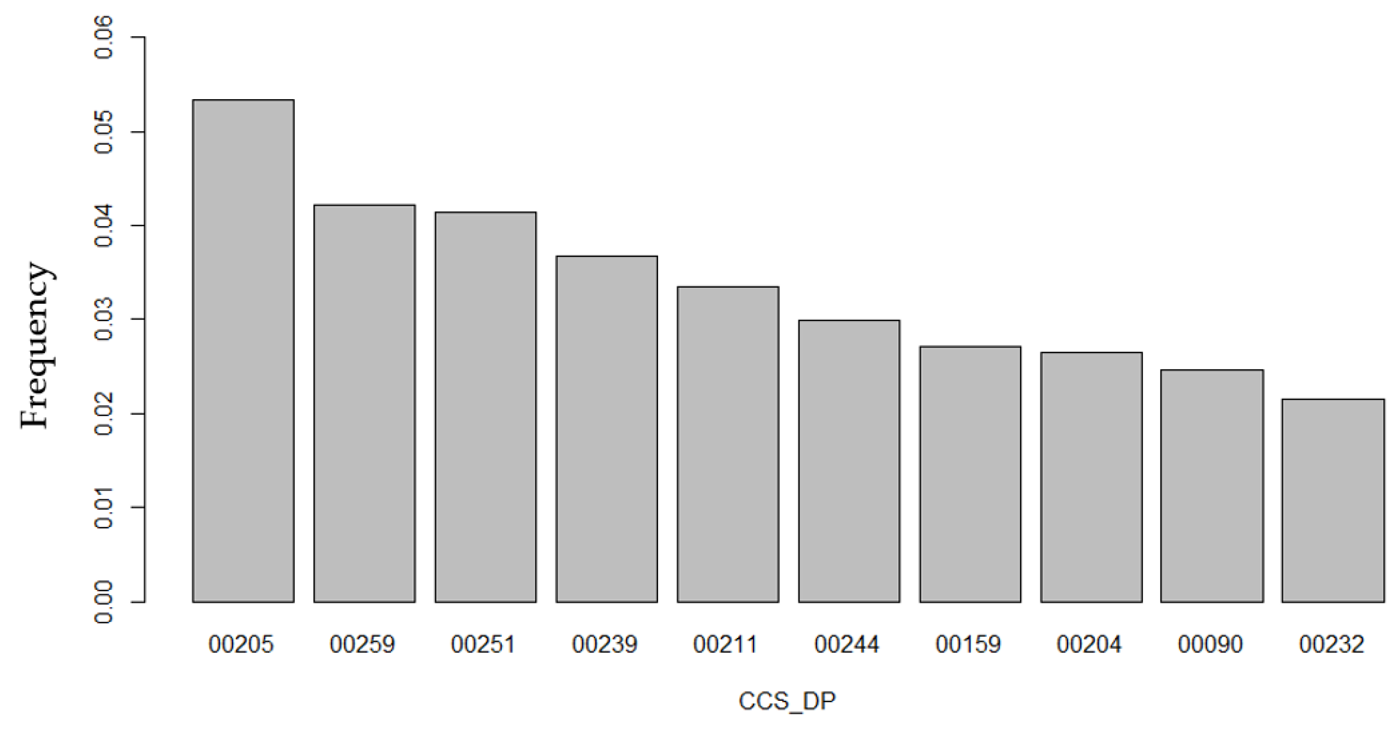
The most predominant symptoms classified at arrival of the patient in the ED were (
Figure 8): spondylosis, intervertebral disk disorder, and other back complaints (4.43%, 141,357 observations), followed by superficial wound and concussion (4.23%, 134,970 observations), abdominal pain (4.12%, 131,261 observations), non-classified codes for causes that were unclear, not included in the CCS or that the patient could not describe (3.96%, 126,190 observations), and other respiratory infections in the upper tract (3.65%, 116,420 observations).
On the other hand, the top five symptoms leading to a higher percentage of admitted patients were polyhydramnios and other disorders in the amniotic cavity with a 92.0% of the visits ending in admission (6145 observations), followed by appendicitis and other appendicular affections, with an admission rate of 88.2% (5633 observations), non-diabetic pancreatic disorders with 87.1% (3864 observations), umbilical cord complications with 87.0% (31 observations), and finally, femoral neck fracture showed an 86.9% admission rate (7073 observations).
4.2. Model Performance
4.2.1. Complete Dataset
The first model analyzed was developed with the complete dataset, including all the observations deemed valuable (see
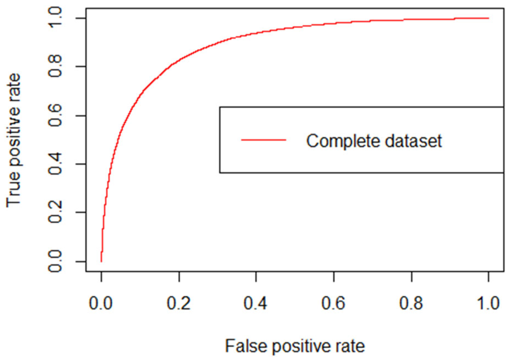
Figure 3 in Data Preparation). The accuracy of the model was 0.9113, exceptionally high when compared to the results obtained by other studies. The AUC for this model obtained from the ROC curve was 0.8938 with a 95% CI of 0.8929–0.8948, also a better result than any observed at the time of arrival to the ED in any previous study.
Figure 9 shows the ROC curve obtained for this first model, varying the discrimination threshold from 1 (bottom left corner) to 0 (upper right corner). As always sought in ROC curves, the objective is to have the curve as close to the upper left corner as possible, which implies a high true positive rate (sensitivity), with a low false positive rate (1—specificity). All the ROC curves for the following models had the same shape, so they have not been included in the report to avoid repetition.
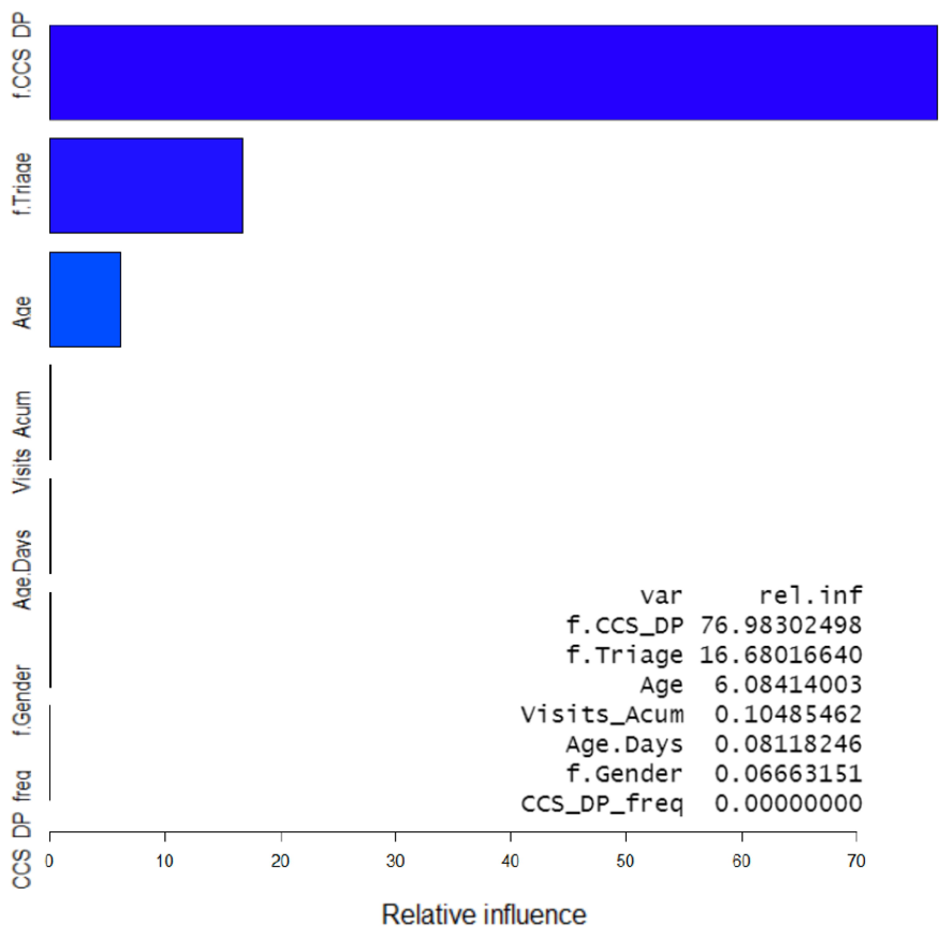
The importance of the variables in the model was obtained with the summary function of the “gbm” package and it showed that the symptom classified with the CCS method was the variable providing the higher information gain at every tree split (76.98%), followed by the triage level (16.68%) and age (6.08%). The four remaining variables (accumulated number of visits during the year, days of age for babies, gender, and frequency of appearance for CCS symptoms) had an almost non-significant contribution to the model adding up to 0.25% of the explanation of it, with the frequency of CCS symptoms showing a null relative influence. This information was used to create a model including only the first three variables and to run the analysis again. This yielded results similar to these of the complete model, with an accuracy of 0.9112 and an AUC of 0.8936 (95% CI 0.8927–0.8946). Variable importance is shown in
Figure 5.
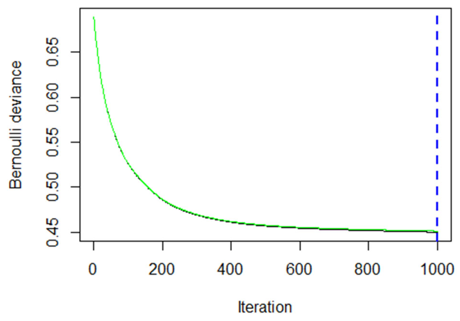
The initial model was tested for overfitting, but the results clearly showed that using three levels of depth for the trained trees and a 0.01 shrinkage parameter, 1000 trees were an optimal amount and not large enough to run into overfitting.
Figure 10 shows the error on both the train (black line) and test (green line) subsets. It is clear that the performance on the test set is not being jeopardized by overfitting to the training set characteristics. The dotted blue line shows the optimal number of iterations (trees) given the input parameters.
4.2.2. Pediatrics Dataset
This subset included all the observations of patients from 0 to 17 years of age inclusive, which added up to 687,288 observations of 381,470 different patients. This model provided an accuracy of 0.9577, with an AUC of 0.8703 (95% CI 0.8667–0.8739). Note that this model has higher accuracy but lower AUC than the complete dataset; this is an indicator of this model being very good at identifying discharges but not so good at identifying admissions, which is probably a consequence of a very imbalanced set in terms of the ratio of admissions/discharges. The importance of the variables in this model differed from that observed in the complete dataset as well, with symptoms and triage still occupying the first and second places (69.13% and 25.97%, respectively), but with days of age in the third position (3.02%) right in front of age in years (1.79%).
4.2.3. Adults Dataset
This subset included 2,501,916 observations from 1,425,606 unique patients ranging from 18 to 115 years of age. The predictive model obtained had an accuracy of 0.8985 and an AUC of 0.89112, with a 95% CI of 0.8901–0.8922. Variable importance for this model showed the same rank as for the complete dataset with slightly different contributions; 79.95% for CCS symptoms, 15.25% for triage, and 4.54% for age.
4.2.4. Young Adults Dataset (between 18 to 70 Years Old)
The young vs. old adult division was performed to test the results obtained by Lucke, J.A. et al. (2018) [
29]. This one included 1,819,221 observations from 1,070,125 different patients and provided an accuracy of 0.9292. The AUC for this subset was 0.89114 with a 95% CI of 0.8896–0.8926. The most important variable was, again, CCS symptoms (81.29%), followed by triage (16.26%) and age (1.81%).
4.2.5. Old Adults Dataset (over 70)
The second adult subset included 682,695 observations from 357,913 unique patients. The predictive model developed provided an accuracy of 0.8182 with an AUC of 0.8514 (95% CI 0.8496–0.8533), clearly ranking last in performance among all subsets. Variable importance consistently showed CCS symptoms as the most informative variable, with triage and age occupying the second and third places (85.64%, 13.36%, and 0.765%, respectively).
Table 3 presents the summary of models’ performance results in different kinds of datasets.


