Featured Application
The proposed solution provides a quick approach for the annotation of the necessary training data to create an application-specific machine learning model that can be used to annotate medical image studies.
Abstract
A major obstacle to the learning-based segmentation of healthy and tumorous brain tissue is the requirement of having to create a fully labeled training dataset. Obtaining these data requires tedious and error-prone manual labeling with respect to both tumor and non-tumor areas. To mitigate this problem, we propose a new method to obtain high-quality classifiers from a dataset with only small parts of labeled tumor areas. This is achieved by using positive and unlabeled learning in conjunction with a domain adaptation technique. The proposed approach leverages the tumor volume, and we show that it can be either derived with simple measures or completely automatic with a proposed estimation method. While learning from sparse samples allows reducing the necessary annotation time from 4 h to 5 min, we show that the proposed approach further reduces the necessary annotation by roughly 50% while maintaining comparative accuracies compared to traditionally trained classifiers with this approach.
1. Introduction
The identification or semantic segmentation of regions of interest (ROIs) in medical images is a common prerequisite for image-based medical studies. The manual creation of such segmentation is often not only time- and cost-intensive but also subject to intra- and inter-rater variability—which drives a need for automatic segmentation methods [1,2,3]. However, there is a huge range of possible segmentation tasks that differ not only by the actual target structure, i.e., the organ or pathology, but also in the definition of boundaries as well as the imaging modality or contrast. Consequently, existing automatic approaches often need to be adapted to individual use-cases, especially in the case of Magnetic Resonance Imaging (MRI). The high variability of this imaging modality with the possibility for individual selection and configurations of MRI sequences together with the manufacturer and device-specific imaging must be accounted for to obtain robust solutions [4,5].
Machine-learning-based approaches are currently considered the state-of-the-art solution for medical image segmentation as they combine strong performance and a straightforward adaptation to new tasks. Solutions such as the deep-learning-based nn-Unet have been successfully applied to a wide range of different problems by adapting the training data to each task [6,7,8]. However, annotating a training dataset can already require significant efforts that might not be justified for a single application. A solution to this challenge is the use of weakly supervised learning, i.e., not using a direct one-to-one annotation for all observations [9,10]. Different approaches have been proposed to reduce the annotation load by employing only incomplete or sparse annotations during the training process [11,12]. This increases the annotation speed and allows the usage of learning-based solutions even for single-time usage.
A limitation of weak supervision with sparse annotations is the missing implicit information about background tissue. If the complete region of interest is segmented, anything not annotated can be considered as the background or the negative class. This is not true if the annotation is incomplete as both positive and negative parts are not annotated, and approaches such as [11] required the annotation of both background and foreground regions. We want to improve this situation by only allowing the annotation of the region of interest, which leads to a situation that resembles the learning from positive and unlabeled data scenarios (PU-learning). Here, the majority of data are unlabeled, and only a few samples from the positive or foreground class are annotated. Different deep-learning based approaches using PU-learning has been proposed for medical imaging analysis tasks [13,14] so far. While deep-learning and the included feature learning is particularly beneficial for large datasets [15], image-based medical studies are often based on small datasets [16]. This creates a need for data-efficient learning. Using traditional machine learning with either hand-crafted or pretrained features can be a solution to this challenge. We, therefore, investigated the combination of PU-learning and random-forest-based image segmentation, as this type of classifier has shown to be efficient for medical image segmentation [17,18,19,20,21,22]. As a foundation, the DALSA (Domain Adaptation for Learning from Sparse Annotations) algorithm is used, providing an intuitive approach for the incorporation of sparse annotations and is already being applied to small imaging datasets [23,24]. We extended this approach to learn from tumorous annotations only and avoiding the creation of labels for the background tissue. The segmentation of brain tumor was selected as an evaluation task with tumorous tissues being the foreground or the positive class and unaffected/healthy tissue being the background/negative class. Our main contributions are as follows:
- A random-forest based PU-learning algorithm for medical image data segmentation;
- A class-prior estimation algorithm with integrated domain-shift correction;
- A image-wise batch-mode for PU-learning;
- A study-based assessment of different tumor volume estimation approaches.
2. Methods
A machine-learning-based workflow for automatic medical image segmentation is proposed based on sparse and positive-only labels. The approach is based on the DALSA approach proposed by [12]. Similarly to this approach, random forests are chosen as classifiers due to their successful application in medical image segmentation in previous studies. Figure 1 provides an overview over the proposed workflow that is evaluated in the case of tumor segmentation.
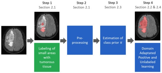
Figure 1.
Training workflow of the proposed segmentation algorithm with sparse positive annotations only. Except for step 1, all steps can be fully automated. The trained classifier is identical to a classifier trained with conventional annotations and can be used without any manual interaction.
The basic approach is a voxel-wise classification approach. Each voxel is represented by a feature vector, . Using a dedicated training dataset, a random forest classifier is trained to classify new voxels into different tissue types. As we build our work on the DALSA approach, the training data are only sparsely annotated (cf. Section 2.1), and all labeled voxels are used for the training process. As a consequence of this annotation process, the training must be corrected to account for and avoid a bias, which is achieved by using voxel-wise weights (cf. Section 2.4). We extend this approach by only allowing the use of positive annotations during training. This requires an additional correction weight, which is calculated based on the ratio of the available classes (cf. Section 2.2). Consequently, the class ratio must be estimated (cf. Section 2.3). Neither the original DALSA nor our approach requires adaptations during the test routine. Instead, segmentations are created simply by classifying all voxels using the previously trained random forest classifier.
2.1. Labeling and Preprocessing
The annotation process is sped up by allowing the annotation of only small portions of the image. There are no hard limitations regarding size, the number of different areas, or location as long as the selected areas are representative and cover the foreground tissue. In the given case, the followiing methods were attempted: (1) all appearances of the tumorous tissue were covered; (2) border voxels are included if they clearly belong to tumors; (3) no unclear areas are marked. There is no spacial limitations about the annotated areas but they are typically located only in one or two slices of each 3D volume. Figure 2 shows examples of the obtained annotations.

Figure 2.
Four example slices from volumes of the in-house dataset that contain sparse and positive annotations. Most other slices of the volumes are annotation-free; at most one or two contain smaller additional annotations. The non-affected tissue is not annotated.
In contrast to the annotations used in [12], the creation of background (healthy) annotations was omitted. As a consequence, the training data contained only tumorous labeled (positive training samples with ) and unlabeled voxels (unlabeled training samples ), which could be either healthy or tumorous tissue. Therefore, traditional semi-supervised learning methods, such as [25], could not be used as they would also require some labeled samples of healthy tissue, i.e., negative training samples (). Instead, a specific approach for learning from such weak annotations is required.
2.2. Learning from Positive Samples
The underlying idea of the proposed approach is to use the proxy task for predicting the availability of a label for a data point and adapting it to the given classification task. A classifier is trained to infer the probability of whether a data point is labeled () or not (). Elkan et al. showed that it is possible to convert this training by introducing class-costs during the training so that the final classifier predicts a given sample label y instead of labeling property s [26]. During the training of a cost-based classifiers, each class is assigned a specific cost for miss-classification, providing an effective method to control the class sensitivity of a classifier [27].
The idea behind this approach is visualized in Figure 3 for an idealistic case with clearly separable classes. As only positive samples are annotated, the probability of annotation should be zero for negative samples and corresponds to the fraction of annotated positive samples for positive samples. If the importance of annotated samples increased so that the increased number of annotated samples matches the overall number of positive samples in the image, the probabilities match the class probability. This is of course a simplified example, assuming clear separability between the classes. However, the same underlying idea also works for non-trivial problems.
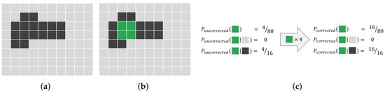
Figure 3.
Schematic explanation of the idea behind weight-based PU-learning. (a) Original image: The bright and dark pixels of the image represent its two classes. (b) Original image with segmentation overlayed: The green pixels show that the sparsely annotated areas are the sparse annotations. (c) Probability of the green class: The probability of annotations given for different preconditions. If the weight for annotated pixels artificially increased, the annotation probability matches the original class probability.
For PU-learning, costs factors and of the positive and the unlabeled class depend on the class prior as well as the positive sampling rate with n and being the numbers of labeled and unlabeled voxels, respectively. They are chosen in a way that the classification error for the classifier is minimized for the estimation of observation labels. We used, in our experiments, costs similar to the ones proposed by Plessis et al., while accounting for the greedy optimization strategy of random forests and the convex loss function [28].
A common assumption in PU-learning is that the class and sampling ratios are constant for all observations, and as a consequence, costs are calculated for all samples of one class. We call this mode the ’global mode’, reflecting the fact the weights are calculated globally for all samples. However, the visible fraction of the tissue type in a image can be variable, and as a consequence, we interpret each image as an individual group of observations or batch. This allows the calculation of individual weights per image, meaning that the class’ cost depends on the image and not on the entire training dataset; we denote this approach as the ’batch mode’.
2.3. Estimating Missing Class Priors
Usually, the ratio of foreground and background or positive and negative is unknown and needs to be either manually or automatic heuristically estimated. For some medical tasks, manual estimation procedures exist while they are not known to other tasks. We therefore evaluated both a manual and an automatic estimation of the class prior. For this study, the class prior corresponds to the ratio of gross tumor volume (GTV) to the volume of healthy tissue in the unlabeled data, which can be derived from a completely segmentation of tumorous tissue using the ratio of GTV-labeled voxels vs. other voxels. However, it is not possible to use this approach when given only incomplete annotation, and other methods are needed to estimate .
The automatic estimation of : might be estimated from the data assuming that positive and negative data are different enough and that the positive samples are drawn independently and are identically distributed (i.i.d). Du Plessis et al. proposed estimating this ratio by finding the overall class prior that reduces the difference between the two distributions and [29]. The intuition behind this is that parts of the original distribution that are caused by the positive samples will be matched, while the other parts cannot be matched. This concept is schematically illustrated in Figure 4a,b.
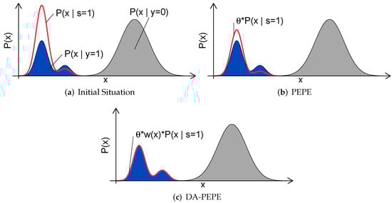
Figure 4.
Schematic depiction PEPE and DA-PEPE (cf Section 2.2). (a) Initial situation: Colored area represents the density of the unlabeled data, with blue representing the positive data and gray representing the negative. The density of the sampled data is represented by the bold red line. (b) PEPE: is chosen to minimize the distribution of annotated and unlabeled data. (c) DA-PEPE: Applying domain adaptation allows a more accurate estimation of in the case of sampling bias.
Du Plessis et al. suggest using Pearson divergence (PE) to measure the similarity of both distributions and to derive an analytic solution for . We refer to this method as ‘Pearson Divergence Prior Estimation’ (PEPE) and calculate based on it as follows.
An underlying assumption for PEPE is that positive samples are drawn i.i.d [29]. However, the manual sparse annotation process always nearly leads to a sampling bias that might affect the performance of the estimation algorithm (cf. Figure 4b). We therefore propose to include a correction of the sampling bias by using importance weighting [30]. Here, the idea is to weight each sample with an sample-dependent weight factors so that the corrected distribution matches the original distributions from which the data have been drawn. To achieve this, each sample is weighted accordingly to the following ratio (cf. Equation (5)):
by correcting the positive class estimation according to the following.
The weighting factor must be estimated since the computational estimation of a distribution is challenging and neither nor are known. We use the estimation approach that is also used for the non-i.i.d correction and that is described in Section 2.4 and call this method the ‘Domain Adapted PEPE’ (DA-PEPE).
Manual estimation of : A manual estimation of is more labor-intensive than an algorithmic estimation and requires an application-specific approach. However, the potentially more accurate estimation and the reduced likelihood for outliers can lead to more accurate classifiers. We, therefore, evaluated two manual estimations of for the given application of brain tumor segmentation based on estimations of the tumor volume with simple manual measurements inspired by common clinical approaches. For the first method, the area of the largest circle fully within tumor is multiplied by the height of tumor . The tumor’s height is obtained by multiplying the slices containing tumors with the slice’s thickness. For the second method, the largest possible diameter, , and the largest perpendicular diameter within the same slice, , were measured, and the tumor volume was estimated by .
2.4. Correction for Non-i.i.d Data
The small and incomplete image annotations covering the image’s content usually are not in an i.i.d. fashion. Consequently, the annotated training and test data follow different distributions and , leading to sub-optimal decision boundaries. This situation, referred to as a sampling bias, leads to a reduced performance of the so-trained classifier [12]. Based on the original DALSA approach, we are correcting this sampling bias by weighting each training point with [12,31]. The weights are chosen to ensure that training and test distribution are equal.
The estimation of w is a non-trivial task that requires the estimation of two density distributions. A possibility to surrogate the direct estimation of the distributions is to train a probabilistic classifier to differentiate between annotated and non-annotated data. The inferred probability for an observation to be annotated, , can then be used to estimate the correct weighting factor by using the following.
If a logistic regression classifier with is used, this formula can be further simplified into a numerically more stable version. Using the learned parameter of the logistic regression , it then becomes the following.
2.5. Benchmark Methods
To evaluate our method, we implemented two baseline methods. First, we trained the classifier using complete segmentation (Complete), as it is usually performed. As a second method, we trained the classifier not only on positive but also on negative samples (SPN) and corrected for occurring sampling errors using domain adaptations [12].
3. Experiments and Results
Two datasets have been used for the experiments. An explorative analysis was conducted using an in-house dataset of 19 patients with glioblastoma. For this in-house dataset, T1 contrast-enhanced, T2 Flair- and diffusion-tensor (DTI)-MRI images are available for each subject. More details on imaging parameters are provided in [12]. The images were rigidly registered to the Flair image and resampled to a common in-plane spacing of 1 mm × 1 mm. A brainmask was extracted semi-automatically and T1 and T2 images were normalized to a standard deviation of 1 and a mode of 0. The image intensity at each voxel and different DTI-derived measures were used as features corresponding to the approach described in [12].
Trained experts manually segmented the GTV and used images from earlier or later timepoints for the iterative improvement of segmentations. This careful labeling process of the ground truth took more than four hours per subject. In addition to the small and only positive (tumorous) regions, a trained radiologist also created small annotations of healthy tissue (negative regions) to allow training the benchmark method. The creation of the small samples for all classes took less than 5 min per patient. The sparse annotations covered 0.25% ± 0.15% of the complete brain volume and 2.6% ± 1.5% of tumorous tissues. Of the sparse annotated voxels, 55.1% ± 16.5% belonged to negative samples.
In addition to this, the BraTS 2013 dataset [32] was used for validation in an independent cohort. To avoid overengineering, only final experiments were conducted using the BraTS dataset. Thus, if not stated otherwise, the in-house dataset was used.
The BraTS 2013 dataset was preprocessed accordingly to [17] as a strong baseline approach. The images were normalized using histogram matching based on a 3D-Slicer [33]. The contrast of an arbitary subject (HG0001) was used as the reference. All voxels with intensity below the mean image intensity were discarged as background images. Follwoing this step, all images were normalized to the mean intensity of the CSF. For this, CSF was semiautomatically segmented in all subjects. The original four modalities were extended to ten images per subject by subtracting each contrsat from the others. For each image in the stack, the Laplacian of the Gaussian (scale 1.0) of the structure’s tensor eigenvalues (scale 1.6) and the Hessian of Gaussian eigenvalues (scale 1.6) were calculated and used together with the pure intensities as features.
3.1. Estimation of
The estimation of the is a crucial step in the proposed approach. We therefore evaluated the quality of the two manual and two algorithmic estimation methods by comparing them to the class prior for each patient that was estimated on the basis of the reference segmentation (Table 1). The algorithmic estimation, which requires no manual interaction, was less accurate and underestimated the tumor prior. Both algorithmic approaches produced one outlier for the same patient. A visual inspection of the images of the corresponding subject revealed a low contrast between tumorous to healthy tissues. Without this outlier, Pearson’s correlation coefficients between the estimated and reference class prior were and for PEPE and DA-PEPE respectively. We kept the outlier within our training base for further experiments.

Table 1.
Estimations of class prior and the correlation between the reference ratio and the estimation.
We analyzed the influence of on the final segmentation result by running multiple leave-one-out experiments with artificially falsified class priors both for the global and batch mode (Figure 5). In general, both modes were stable against incorrectly estimated and were more robust against overestimation than underestimation.
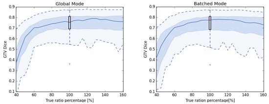
Figure 5.
Results of leave-one-out experiments with artificially falsified . All experiments are conducted with the same random forest tree depth (Global 5 and Batched 4).
3.2. Segmentation Results
We ran leave-one-out experiments with all 19 subjects to evaluate our method with respect to benchmark methods. We also compared the proposed batched mode vs. the global mode. We chose the well-known DICE score [34] as the metric for the evaluation of the classifier’s results to ensure comparability with other studies. Following the reasoning of Menze et al., we excluded distance measures [32]. Figure 6 shows the obtained DICE score for each method.
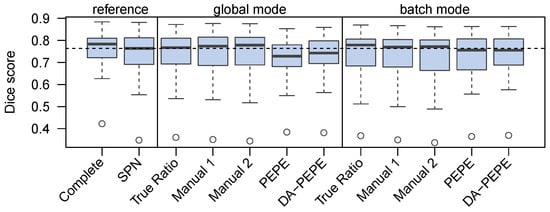
Figure 6.
DICE scores for different leave-one-out configurations. All experiments except ’complete’ used importance weighting. The horizontal dashed line shows the median of the current state-of-the-art method.
Given reference , the proposed workflow yielded classifiers that are comparable to learning from positive and negative samples (SPN). Compared to the reference-prior-based classifier, the results improved when manual estimation was used in the batch mode. Generally, batch-mode training provided better results than global mode training. There was a small drop in the quality of results when using the automated estimation of . However, the retrieved DICE scores were still comparable to the state-of-the-art methods that used both positive and negative labels.
DA-PEPE provides slightly better results than PEPE even though it has a less favorable correlation coefficient and a higher mean error. We think that this is because it overestimated low and generally performed better for high . Since the proposed workflow is less sensitive to overestimation, the so-made estimation error might lead to improved results.
3.3. Validation on the Second Dataset
To validate the proposed approach on a independent dataset the proposed PU-learning strategy was tested on the BraTS 2013 dataset. Sparse positive annotations were created, corresponding to the ones on the in-house dataset, and the DA-PEPE approach was used to estimate . As the dataset contains multiple labels, we used a multi-class classification, also showing that the proposed approach can be used with more than two classes. We therefore created only annotations of affected tissue, and the largest type of non-affected tissue (background) was left unannotated.
The obtained mean DICE score from leave-one-out experiments is 78.7% ± 15.7%, and the sensitivity and specificity are 78.3% ± 15.9% and 98.8% ± 1.2%, respectively. These results are inline with the expected results from other experiments and could be further improved using more sophisticated features and additional post-processing [17]. Figure 7 shows some examples of the obtained segmentation, both as two and multiclass results.
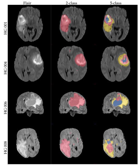
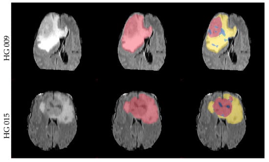
Figure 7.
Example axial and coronal (HG 006) slices from the validation set u(BraTS 2013 dataset) using the proposed PU-learning method. The colour coding is as follows: ‘yellow’: edema; ‘red’: enhancing tumour; ‘green’: non-enhancing tumour; ‘blue’: necrosis. The subject name is identical to the identifier within the original training dataset.
4. Discussion
We showed that the proposed approach allows for the training of an effective tumor segmentation algorithm from small and only positive samples. The approach dramatically reduces the labeling time when compared to the traditional workflow with training on complete segmentations. The results achieved by such a classifier are comparable or better than those achieved by learning from sparse positive and negative samples (SPN), while the required labeling time is further reduced—for our experiments, by nearly . This will enable the creation and regular update of much larger training sets than previously employed, making it much easier to directly integrate the approach in a clinical workflow and to cover different scanner hardware, modalities, protocols, and even different clinical applications.
Using a cost-based approach allows the combination of our method with most learning-based approaches, making it more general than previous methods such as [35]. Nevertheless, there are some difficulties in incorporating spacial priors from an atlas. However, instead of using a spacial prior, a tissue class prior can be derived for each voxel and a general tumor probability can be used for post-processing the segmentation. This allows the use of most information encoded within an atlas, although there are enough methods that obtain good results without using this information (for example, [17,36]).
For this paper, we purposely used simple features and classifiers in order to deflect attention to such details. However, given the flexibility of the proposed approach with the cost-based classifier as the only real requirement, the performance can be easily improved. For example, by using more advanced technology stacks, including the usage of deep learning. This could be by using learned features from a pretrained network [37], a combination of forest and deep learning [38], or a cost-sensitive deep segmentation network [39]. These changes will not affect the ability of the baseline approach proposed here to be trained from sparse and positive-only annotations and can improve the performance’s results significantly.
One benefit of PU-learning is that the estimation of the tissue ratios can be obtained with multiple approaches. The best approach depends on the use-case; for example, if the true tissue ratio is known from a previous study or a post-surgical histological measurement, those could be used without any additional overhead. However, even if such accurate measures are unavailable, PU-learning can still be used, as our experiments show that it is robust even with an estimation error of , which allows the usage of quick but less accurate estimation methods for the reduction in annotation loads.
The best manual estimation of tissue ratios depends on the actual task on hand. In our experiments, these measures showed a tendency to overestimate the tumor volume by and percentage points (cf. Table 1), which is in line with other findings suggesting a slight overestimation of tumors using simple measurements [40]. However, these approaches were shown to be sufficiently accurate and might already be assessed in clinical routines [41], thus offering a good alternative. However, there might be cases when manual estimations are unavailable and cannot simply be created, either because of time and cost restrictions or because it is simple not possible for the given task. In such settings, the heuristic estimation of the tumor volume is a possible alternative. While the accuracy of such estimations is lower than the accuracy of manual estimations, the performance is still sufficient for training high-quality classifiers with performances that are on par with those of other solutions (cf. Figure 6. This is true especially if the proposed batch mode is used for the training.
The labeling process—an important part of this method—raises questions about the observer dependency of the process, the best amount of data to be labeled, and the best location for the labels. Preliminary results, which would exceed the scope of this work, indicate that the method is generally robust against different labeling. Further efforts will be undertaken in the future to investigate this in more detail.
The results on the external validation set also showed that it is possible to extend PU-learning to a multi-class setting by leaving only one class aside. Similarly to a two-class problem, the proportion of each class is then estimated either manually or heuristically, and the classifiers are corrected accordingly. The flexibility by this process allows the adaptation of the proposed technique to a wide range of different tasks.
The recent rise of radiomics drives additional needs for image segmentations. The segmentation of the region of interest is a major step for this approach. While manual segmentation is possible, it is known that the inter-rater variability of such approaches has a major impact on the quality and reliability of the radiomics study [42,43,44,45]. While there are methods to control for the influence of rater variability from the segmentations [45,46], the usage of automatic segmentations is often considered better as the transfer to other clinical settings is more straightforward [47]. While there are some studies that make use of automatic segmentations [48,49], this is not always true. We assume that the comparatively small size of many studies [16,50,51] hinders the researcher in investing additional efforts. However, given the original capabilities of the baseline, we expect that our solution can provide an easy approach to develop automatic segmentation solutions even with limited data.
Our solution requires less annotated data compared to traditional semi-supervised learning methods. These methods usually require the annotation of both healthy and tumorous tissue, which might be a problem for crowd-sourcing-based labeling. Having two different tasks either doubles the number of tasks that needs to be solved or requires switching the current label. Employing a weak supervision with PU-learning, this situation is avoided with our method. This might be particularly useful in settings where switching the annotation is costly (for example, if crowd-sourcing is used [52,53]). In this setting, the simplified annotation can be even more beneficial, as the non-expert crowd annotator is not required to fully comprehend all details of the image and can accomplish each task faster, which further reduces the cost.
This research is an important step towards fast annotations for automatic studies. This allows leveraging the benefits of automatic segmentation approaches even in smaller medical studies, which will no longer need to depend on manual segmentation. This improves the reliability and reproducibility of such studies that can build on this solution. However, there is still room for further improvements on this topic: for example, by incorporating deep-learning-based approaches to the suggested solutions or by evaluating it usefulness directly in a medical study.
Overall, the proposed workflow can reduce and simplify the labeling effort in the field of automatic tumor segmentation. This is an important step in order to be able to include tumor segmentation into a general clinical workflow.
Author Contributions
Conceptualization, D.W. and M.G.; methodology, M.G.; validation, M.G.; formal analysis, M.G.; investigation, M.G.; resources, R.T., B.B.-B., J.P. and M.G.; data curation, S.R., R.T., B.B.-B., J.P. and M.G.; writing, D.W. and M.G.; project administration, M.G. All authors have read and agreed to the published version of the manuscript.
Funding
This research was funded by the University of Ulm grant number L.SBN.0214.
Institutional Review Board Statement
This retrospective single-institution study was approved by the local ethics committee (Bioethics Committee of Medical University of Silesia in Katowice) and conducted in agreement with the declaration of Helsinki.
Informed Consent Statement
Due to the retrospective nature of the study, written informed consent was waived.
Data Availability Statement
The data presented in this study are available on request from the corresponding author. The data are not publicly available due to privacy and ethical restrictions.
Acknowledgments
We would like to thank the late Franciszek Binczyk, who sadly passed away far too young. He contributed significantly to this study, which would have not been possible without him.
Conflicts of Interest
The authors declare no conflict of interest.
Abbreviations
The following abbreviations are used in this manuscript:
| ROI | Region of interest; |
| MRI | Magnetic resonance imaging |
| PU-learning | Learning from positive and unlabeled data; |
| DALSA | Domain adaptation for learning from sparse annotations; |
| GTV | Gross tumor bolume; |
| PE | Pearson divergence; |
| PEPE | Pearson divergence prior estimation; |
| DA-PEPE | Domain-adapted Pearson divergence prior estimation; |
| i.i.d | Independently and identically distributed; |
| DTI | Diffusion tensor imaging; |
| CSF | Cerebrospinal fluid; |
| SPN | Learning from sparse positive and negative samples. |
References
- Perthen, J.E.; Ali, T.; McCulloch, D.; Navidi, M.; Phillips, A.W.; Sinclair, R.C.F.; Griffin, S.M.; Greystoke, A.; Petrides, G. Intra- and interobserver variability in skeletal muscle measurements using computed tomography images. Eur. J. Radiol. 2018, 109, 142–146. [Google Scholar] [CrossRef] [PubMed]
- Kocak, B.; Durmaz, E.S.; Kaya, O.K.; Ates, E.; Kilickesmez, O. Reliability of Single-Slice–Based 2D CT Texture Analysis of Renal Masses: Influence of Intra- and Interobserver Manual Segmentation Variability on Radiomic Feature Reproducibility. Am. J. Roentgenol. 2019, 213, 377–383. [Google Scholar] [CrossRef] [PubMed]
- Götz, M.; Nolden, M.; Maier-Hein, K. MITK Phenotyping: An open-source toolchain for image-based personalized medicine with radiomics. Radiother. Oncol. 2019, 131, 108–111. [Google Scholar] [CrossRef] [PubMed]
- Bendfeldt, K.; Hofstetter, L.; Kuster, P.; Traud, S.; Mueller-Lenke, N.; Naegelin, Y.; Kappos, L.; Gass, A.; Nichols, T.E.; Barkhof, F.; et al. Longitudinal gray matter changes in multiple sclerosis—Differential scanner and overall disease-related effects. Hum. Brain Mapp. 2012, 33, 1225–1245. [Google Scholar] [CrossRef]
- Hammarstedt, L.; Thil er-Klang, A.; Muth, A.; Wängberg, B.; Odén, A.; Hellström, M. Adrenal lesions: Variability in attenuation over time, between scanners, and between observers. Acta Radiol. 2013, 54, 817–826. [Google Scholar] [CrossRef]
- Isensee, F.; Jaeger, P.F.; Kohl, S.A.A.; Petersen, J.; Maier-Hein, K.H. nnU-Net: A self-configuring method for deep learning-based biomedical image segmentation. Nat. Methods 2021, 18, 203–211. [Google Scholar] [CrossRef]
- Deike-Hofmann, K.; Dancs, D.; Paech, D.; Schlemmer, H.P.; Maier-Hein, K.; Bäumer, P.; Radbruch, A.; Götz, M. Pre-examinations Improve Automated Metastases Detection on Cranial MRI. Investig. Radiol. 2021, 56, 320–327. [Google Scholar] [CrossRef]
- Hatamizadeh, A.; Tang, Y.; Nath, V.; Yang, D.; Myronenko, A.; Landman, B.; Roth, H.R.; Xu, D. UNETR: Transformers for 3D Medical Image Segmentation. In Proceedings of the IEEE/CVF Winter Conference on Applications of Computer Vision (WACV), Waikoloa, HI, USA, 3–8 January 2022; pp. 574–584. [Google Scholar] [CrossRef]
- Roth, H.R.; Yang, D.; Xu, Z.; Wang, X.; Xu, D. Going to Extremes: Weakly Supervised Medical Image Segmentation. Mach. Learn. Knowl. Extr. 2021, 3, 26. [Google Scholar] [CrossRef]
- Chan, L.; Hosseini, M.S.; Plataniotis, K.N. A Comprehensive Analysis of Weakly-Supervised Semantic Segmentation in Different Image Domains. Int. J. Comput. Vis. 2021, 129, 361–384. [Google Scholar] [CrossRef]
- Goetz, M.; Weber, C.; Stieltjes, B.; Maier-Hein, K. Learning from Small Amounts of Labeled Data in a Brain Tumor Classification Task. In Proceedings of the NIPS Workshop on Transfer and Multi-task learning: Theory Meets Practice, Montreal, QC, Canada, 13 December 2014. [Google Scholar]
- Goetz, M.; Weber, C.; Binczyk, F.; Polanska, J.; Tarnawski, R.; Bobek-Billewicz, B.; Koethe, U.; Kleesiek, J.; Stieltjes, B.; Maier-Hein, K.H. DALSA: Domain Adaptation for Supervised Learning From Sparsely Annotated MR Images. IEEE Trans. Med. Imaging 2016, 35, 184–196. [Google Scholar] [CrossRef]
- Li, L.; Wei, M.; Liu, B.; Atchaneeyasakul, K.; Zhou, F.; Pan, Z.; Kumar, S.A.; Zhang, J.Y.; Pu, Y.; Liebeskind, D.S.; et al. Deep Learning for Hemorrhagic Lesion Detection and Segmentation on Brain CT Images. IEEE J. Biomed. Health Inf. 2021, 25, 1646–1659. [Google Scholar] [CrossRef] [PubMed]
- Lejeune, L.; Sznitman, R. A positive/unlabeled approach for the segmentation of medical sequences using point-wise supervision. Med. Image Anal. 2021, 73, 102185. [Google Scholar] [CrossRef] [PubMed]
- Belkin, M.; Hsu, D.; Ma, S.; Mandal, S. Reconciling modern machine-learning practice and the classical bias–variance trade-off. Proc. Natl. Acad. Sci. USA 2019, 116, 15849–15854. [Google Scholar] [CrossRef] [PubMed]
- Kiryati, N.; Landau, Y. Dataset Growth in Medical Image Analysis Research. J. Imaging 2021, 7, 155. [Google Scholar] [CrossRef]
- Kleesiek, J.; Biller, A.; Urban, G.; Kothe, U.; Bendszus, M.; Hamprecht, F. Ilastik for Multi-modal Brain Tumor Segmentation. In Proceedings of the MICCAI-BRATS, Boston, MA, USA, 14 September 2014. [Google Scholar]
- Thayumanavan, M.; Ramasamy, A. An efficient approach for brain tumor detection and segmentation in MR brain images using random forest classifier. Concurr. Eng. 2021, 29, 266–274. [Google Scholar] [CrossRef]
- Csaholczi, S.; Kovács, L.; Szilágyi, L. Automatic Segmentation of Brain Tumor Parts from MRI Data Using a Random Forest Classifier. In Proceedings of the 2021 IEEE 19th World Symposium on Applied Machine Intelligence and Informatics (SAMI), Herlany, Slovakia, 21–23 January 2021; pp. 471–476. [Google Scholar] [CrossRef]
- Mirmohammadi, P.; Ameri, M.; Shalbaf, A. Recognition of acute lymphoblastic leukemia and lymphocytes cell subtypes in microscopic images using random forest classifier. Phys. Eng. Sci. Med. 2021, 44, 433–441. [Google Scholar] [CrossRef]
- Hartmann, D.; Müller, D.; Soto-Rey, I.; Kramer, F. Assessing the Role of Random Forests in Medical Image Segmentation. arXiv 2021, arXiv:2103.16492. [Google Scholar]
- Li, Z.; Feng, N.; Pu, H.; Dong, Q.; Liu, Y.; Liu, Y.; Xu, X. PIxel-Level Segmentation of Bladder Tumors on MR Images Using a Random Forest Classifier. Technol. Cancer Res. Treat. 2022, 21, 15330338221086395. [Google Scholar] [CrossRef]
- Götz, M.; Heim, E.; März, K.; Norajitra, T.; Hafezi, M.; Fard, N.; Mehrabi, A.; Knoll, M.; Weber, C.; Maier-Hein, L.; et al. A learning-based, fully automatic liver tumor segmentation pipeline based on sparsely annotated training data. SPIE Med. Imaging 2016, 9784, 405–410. [Google Scholar] [CrossRef]
- Götz, M.; Skornitzke, S.; Weber, C.; Fritz, F.; Mayer, P.; Knoll, M.; Stiller, W.; Maier-Hein, K.H. Machine-Learning based Comparison of CT-Perfusion maps and Dual Energy CT for Pancreatic Tumor Detection. SPIE Med. Imaging Int. Soc. Opt. Photonics 2016, 9785, 450–455. [Google Scholar] [CrossRef]
- Criminisi, A.; Shotton, J. Decision Forests for Computer Vision and Medical Image Analysis; Springer Science & Business Media: Cham, Switzerland, 2013. [Google Scholar] [CrossRef]
- Elkan, C.; Noto, K. Learning classifiers from only positive and unlabeled data. In Proceedings of the 14th ACM SIGKDD International Conference on Knowledge Discovery and Data Mining, Las Vegas, NV, USA, 24–27 August 2008. [Google Scholar]
- Elkan, C. The foundations of cost-sensitive learning. In Proceedings of the International Joint Conference on Artificial Intelligence, Seattle, WA, USA, 4–10 August 2001. [Google Scholar]
- Du Plessis, M.C.; Niu, G.; Sugiyama, M. Analysis of Learning from Positive and Unlabeled Data. Advances in Neural Information Processing Systems 27. 2014. Available online: https://proceedings.neurips.cc/paper/2014/file/35051070e572e47d2c26c241ab88307f-Paper.pdf (accessed on 4 October 2022).
- Du Plessis, M.C.; Sugiyama, M. Class Prior Estimation from Positive and Unlabeled Data. IEICE Trans. Inf. Syst. 2014, 97, 1358–1362. [Google Scholar] [CrossRef]
- Shimodaira, H. Improving predictive inference under covariate shift by weighting the log-likelihood function. J. Stat. Plan. Inference 2000, 97, 1358–1362. [Google Scholar] [CrossRef]
- Sugiyama, M.; Kawanabe, M. Machine Learning in Non-Stationary Environments: Introduction to Covariate Shift Adaptation; MIT Press: Cambridge, MA, USA, 2012; ISBN 9780262301220. [Google Scholar]
- Menze, B.H.; Jakab, A.; Bauer, S.; Kalpathy-Cramer, J.; Farahani, K.; Kirby, J.; Burren, Y.; Porz, N.; Slotboom, J.; Wiest, R.; et al. The Multimodal Brain Tumor Image Segmentation Benchmark (BRATS). IEEE Trans. Med. Imaging 2015, 34, 1993–2024. [Google Scholar] [CrossRef]
- Kistler, M.; Bonaretti, S.; Pfahrer, M.; Niklaus, R.; Büchler, P. The Virtual Skeleton Database: An Open Access Repository for Biomedical Research and Collaboration. J. Med. Internet Res. 2013, 15, e245. [Google Scholar] [CrossRef] [PubMed]
- Dice, L.R. Measures of the Amount of Ecologic Association Between Species. Ecology 1945, 26, 297–302. [Google Scholar] [CrossRef]
- Prastawa, M.; Bullitt, E.; Ho, S.; Gerig, G. A brain tumor segmentation framework based on outlier detection. Med. Image Anal. 2004, 8, 275–283. [Google Scholar] [CrossRef] [PubMed]
- Pereira, S.; Pinto, A.; Alves, V.; Silva, C.A. Brain Tumor Segmentation using Convolutional Neural Networks in MRI Images. IEEE Trans. Med. Imaging 2016, 35, 1240–1251. [Google Scholar] [CrossRef] [PubMed]
- Jiménez, G.; Racoceanu, D. Deep Learning for Semantic Segmentation vs. Classification in Computational Pathology: Application to Mitosis Analysis in Breast Cancer Grading. Front. Bioeng. Biotechnol. 2019, 7, 145. [Google Scholar] [CrossRef]
- Kontschieder, P.; Fiterau, M.; Criminisi, A.; Bulo, S.R. Deep Neural Decision Forests. In Proceedings of the 2015 IEEE International Conference on Computer Vision (ICCV), Santiago, Chile, 7–13 December 2015; pp. 1467–1475. [Google Scholar] [CrossRef]
- Hou, Y.; Fan, H.; Li, L.; Li, B. Adaptive learning cost-sensitive convolutional neural network. IET Comput. Vision 2021, 15, 346–355. [Google Scholar] [CrossRef]
- Galanis, E.; Buckner, J.C.; Maurer, M.J.; Sykora, R.; Castillo, R.; Ballman, K.V.; Erickson, B.J.; North Central Cancer Treatment Group. Validation of neuroradiologic response assessment in gliomas: Measurement by RECIST, two-dimensional, computer-assisted tumor area, and computer-assisted tumor volume methods1. Neuro-Oncol. 2006, 8, 156–165. [Google Scholar] [CrossRef]
- Jaffe, C.C. Measures of Response: RECIST, WHO, and New Alternatives. J. Clin. Oncol. 2006, 24, 3245–3251. [Google Scholar] [CrossRef] [PubMed]
- Rai, R.; Holloway, L.C.; Brink, C.; Field, M.; Christiansen, R.L.; Sun, Y.; Barton, M.B.; Liney, G.P. Multicenter evaluation of MRI-based radiomic features: A phantom study. Med. Phys. 2020, 47, 3054–3063. [Google Scholar] [CrossRef] [PubMed]
- Wennmann, M.; Bauer, F.; Klein, A.; Chmelik, J.; Grözinger, M.; Rotkopf, L.T.; Neher, P.; Gnirs, R.; Kurz, F.T.; Nonnenmacher, T.; et al. In Vivo Repeatability and Multiscanner Reproducibility of MRI Radiomics Features in Patients With Monoclonal Plasma Cell Disorders: A Prospective Bi-institutional Study. Investig. Radiol. 2022. online ahead of print. [Google Scholar] [CrossRef] [PubMed]
- Van Timmeren, J.E.; Leijenaar, R.T.; van Elmpt, W.; Wang, J.; Zhang, Z.; Dekker, A.; Lambin, P. Test–Retest Data for Radiomics Feature Stability Analysis: Generalizable or Study-Specific? Tomography 2016, 2, 361–365. [Google Scholar] [CrossRef]
- Götz, M.; Maier-Hein, K.H. Optimal Statistical Incorporation of Independent Feature Stability Information into Radiomics Studies. Sci. Rep. 2020, 10, 1–10. [Google Scholar] [CrossRef]
- Orlhac, F.; Boughdad, S.; Philippe, C.; Stalla-Bourdillon, H.; Nioche, C.; Champion, L.; Soussan, M.; Frouin, F.; Frouin, V.; Buvat, I. A Postreconstruction Harmonization Method for Multicenter Radiomic Studies in PET. J. Nucl. Med. 2018, 59, 1321–1328. [Google Scholar] [CrossRef] [PubMed]
- Zwanenburg, A.; Vallières, M.; Abdalah, M.A.; Aerts, H.J.W.L.; Andrearczyk, V.; Apte, A.; Ashrafinia, S.; Bakas, S.; Beukinga, R.J.; Boellaard, R.; et al. The Image Biomarker Standardization Initiative: Standardized Quantitative Radiomics for High-Throughput Image-based Phenotyping. Radiology 2020, 295, 328–338. [Google Scholar] [CrossRef] [PubMed]
- Larue, R.T.H.M.; Defraene, G.; De Ruysscher, D.; Lambin, P.; van Elmpt, W. Quantitative radiomics studies for tissue characterization: A review of technology and methodological procedures. Br. J. Radiol. 2017, 90, 20160665. [Google Scholar] [CrossRef]
- Wennmann, M.; Klein, A.; Bauer, F.; Chmelik, J.; Grözinger, M.; Uhlenbrock, C.; Lochner, J.; Nonnenmacher, T.; Rotkopf, L.T.; Sauer, S.; et al. Combining Deep Learning and Radiomics for Automated, Objective, Comprehensive Bone Marrow Characterization From Whole-Body MRI: A Multicentric Feasibility Study. Investig. Radiol. 2022, 57, 752–763. [Google Scholar] [CrossRef] [PubMed]
- Lisson, C.S.; Lisson, C.G.; Achilles, S.; Mezger, M.F.; Wolf, D.; Schmidt, S.A.; Thaiss, W.M.; Bloehdorn, J.; Beer, A.J.; Stilgenbauer, S.; et al. Longitudinal CT Imaging to Explore the Predictive Power of 3D Radiomic Tumour Heterogeneity in Precise Imaging of Mantle Cell Lymphoma (MCL). Cancers 2022, 14, 393. [Google Scholar] [CrossRef] [PubMed]
- Lisson, C.S.; Lisson, C.G.; Mezger, M.F.; Wolf, D.; Schmidt, S.A.; Thaiss, W.M.; Tausch, E.; Beer, A.J.; Stilgenbauer, S.; Beer, M.; et al. Deep Neural Networks and Machine Learning Radiomics Modelling for Prediction of Relapse in Mantle Cell Lymphoma. Cancers 2022, 14, 2008. [Google Scholar] [CrossRef] [PubMed]
- Maier-Hein, L.; Mersmann, S.; Kondermann, D.; Bodenstedt, S.; Sanchez, A.; Stock, C.; Kenngott, H.G.; Eisenmann, M.; Speidel, S. Can Masses of Non-Experts Train Highly Accurate Image Classifiers? In Medical Image Computing and Computer-Assisted Intervention—MICCAI 2014; Springer: Berlin/Heidelberg, Germany, 2014; pp. 438–445. [Google Scholar] [CrossRef]
- Maier-Hein, L.; Ross, T.; Gröhl, J.; Glocker, B.; Bodenstedt, S.; Stock, C.; Heim, E.; Götz, M.; Wirkert, S.; Kenngott, H.; et al. Crowd-algorithm collaboration for large-scale endoscopic image annotation with confidence. In Medical Image Computing and Computer-Assisted Intervention—MICCAI 2016; Springer International Publishing: Cham, Switzerland, 2016. [Google Scholar] [CrossRef]


Publisher’s Note: MDPI stays neutral with regard to jurisdictional claims in published maps and institutional affiliations. |
© 2022 by the authors. Licensee MDPI, Basel, Switzerland. This article is an open access article distributed under the terms and conditions of the Creative Commons Attribution (CC BY) license (https://creativecommons.org/licenses/by/4.0/).