Abstract
Acute Lymphoblastic Leukemia (ALL) is a cancer that infects the blood cells causing the development of lymphocytes in large numbers. Diagnostic tests are costly and very time-consuming. It is important to diagnose ALL using Peripheral Blood Smear (PBS) images, especially in the initial screening cases. Several issues affect the examination process such as diagnostic error, symptoms, and nonspecific nature signs of ALL. Therefore, the objective of this study is to enforce machine-learning classifiers in the detection of Acute Lymphoblastic Leukemia as benign or malignant after using the grey wolf optimization algorithm in feature selection. The images have been enhanced by using an adaptive threshold to improve the contrast and remove errors. The model is based on grey wolf optimization technology which has been developed for feature reduction. Finally, acute lymphoblastic leukemia has been classified into benign and malignant using K-nearest neighbors (KNN), support vector machine (SVM), naïve Bayes (NB), and random forest (RF) classifiers. The best accuracy, sensitivity, and specificity of this model were 99.69%, 99.5%, and 99%, respectively, after using the grey wolf optimization algorithm in feature selection. To ensure the effectiveness of the proposed model, comparative results with other classification techniques have been included.
1. Introduction
Leukemia is a cancer of the bone marrow that is divided into four types: acute myeloid leukemia (AML), acute lymphoblastic leukemia (ALL), chronic lymphoid leukemia (CLL), and chronic myeloid leukemia (CML). The second most prevalent type of acute leukemia in adults is acute lymphoblastic leukemia. In the bone marrow, it affects lymphocyte-producing cells [1]. The bone marrow and stem cell components are illustrated in Figure 1.
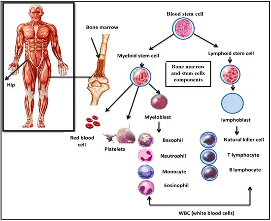
Figure 1.
Bone marrow and stem cells components.
Although ALL is considered one of the leading death causes in both adults and children, nearly 90% of cases can be treated if they can be detected early. When ALL is detected earlier, treatment can begin immediately, and the patient’s chances of survival improve significantly. Several treatment types can be used as medication, radiation therapy, and chemotherapy according to the diagnosis accuracy. Most leukemia diagnosis procedures are manual methods and based on the medical experience of the physicians. The blood cells’ microscopic examinations are an important step in the diagnostic process; this evaluation necessitates the use of a pathologist who is skilled in identifying the abnormalities in the blood cells. One of the most effective tools in medical diagnosis is medical images. According to the extracted features from these images, one can have complete information about medical image contents [2].
Cancer is a group of rare, distinct, and lethal diseases. It can be characterized as uncontrolled cell growth with an abnormal pattern. The World Health Organization (WHO) estimates that 19.3 million people will receive a cancer diagnosis in 2020 and that there will be 1.6 times as many cancer deaths. The number of people affected is expected to be roughly 50% higher in 2040. According to WHO, the total number of ALL cases is 57,377, accounting for 21.9% of all childhood cancer cases worldwide in 2020 [3]. The most well-known leukemia classification system divides acute leukemia types into two groups according to the French–American–British model: acute myeloid leukemia (AML) and acute lymphoblastic leukemia (ALL); the types of leukemia in the blood are shown in Figure 2. The most prevalent cancer types in children are thought to include ALL.
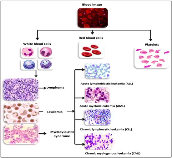
Figure 2.
Types of leukemia in blood.
Indeed, oncologists must identify the most important variables and factors that can be used to predict treatment outcomes. A further classification based on the French–American–British (FAB) classification divides ALL into three subtypes: L1, L2, and L3. L1 cells typically have a small, homogeneous size and little cytoplasm. These organisms have well-structured discoid nuclei. Compared with L1-type cells, L2-type cells are larger and have different shapes. Their cytoplasm is variable, and their nucleus is atypical. L3 cells have a round or oval nucleus and are all the same size and shape. The cytoplasm, which contains vacuoles, is sufficient in them. Usually, they are larger than L1 [3,4].
To predict long-term outcomes or treatment outcomes, numerous studies have been carried out, and almost all of them have used data mining (DM) classifier algorithms, proving the effectiveness and significance of using machine learning techniques for such purposes.
ALL subtypes have been categorized using World Health Organization (WHO) or French–American–British (FAB) techniques; hematologists and dermatologists have recently proposed that WHO categorization is superior to FAB categorization. To more accurately determine the different types of ALL, the WHO classified subgroups in more detail. Researchers from a variety of fields are now interested in using computer technologies such as artificial intelligence (AI) to diagnose blood diseases, particularly ALL. Concerning ALL diagnoses and classifications, the use of these technologies in the form of different algorithms has produced astounding results [5].
1.1. Related Studies
Previous research efforts on leukemia patient classification will be reviewed in this section. Several researchers used microscopic images to propose leukemia detection methods. In [1], deep convolutional neural network (CNN) applications were investigated, and the diagnosis and classification of acute lymphoblastic leukemia, as well as the differentiation between cancer cases and healthy cases, were developed by the authors using pre-trained VGG-16 and ResNet.
Different scenarios were designed for data analysis in [2]. The first scenario includes ALL patients, whereas the second scenario excludes patients who died from an unknown cause from the study. In general, common classification algorithms were used as SVM which showed a significantly improved performance in treatment outcome prediction.
According to the experimental results in [3], CNN was used for automating the ALL-detection task from microscopic cell images. They looked at the weighted ensemble of various deep CNNs in the initial test set to make a better classification model for acute lymphoblastic leukemia cells.
Using the microscopic blood image analysis [4], the authors segmented the image into the basic cell types, such as WBCs (white blood cells), RBCs (red blood cells), and platelets. The lymphocytes are then separated from the white blood cells. The changeable features such as the shape and color of lymphocytes were extracted with a support vector machine as a classifier, which classified the cells as normal or blasts. This detection system was found to be more effective, rapid, and accurate.
In [6], Spark BigDL framework and Google Net architecture were suggested as detection techniques, and it achieved 97.33% accuracy.
Aggregated deep learning for leukemic B-lymphoblast categorization was proposed, as shown in [7]. Data augmentation and transfer learning strategies were used to overcome the limited dataset size and learning speed. The outcomes demonstrated that the suggested method outperformed individual networks in leukemic B-lymphoblast diagnosis by fusing features from the top deep learning models.
A hybrid classification approach for extracting the WBC features was proposed in [8]. The algorithm relies on using a deep convolutional neural network (VGGNet) and filtering the resulting features with a statistically enhanced salp swarm algorithm (SESSA) to extract only relevant features and omit those that are not. The accuracy and complexity reduction of the suggested hybrid approach outperformed those of other approaches, which reduced computation time and resource usage.
In [9], the researchers proposed a deep learning-based automated technique for distinguishing between malignant and benign cells. The use of microscopic blood cell images and CNN to diagnose ALL subtypes of leukemia was proposed by [10].
Several classification techniques were used such as naïve Bayes, SVM, KNN, and decision trees. In [11], AlexNet, GoogleNet, and SqueezeNet were used in the proposed work. The objectives of these structures were to achieve robust, high-accuracy, faster, and more efficient methodology.
In [12], a framework used CNNs. Cell images were used to train the model, extracting the best features after preprocessing the images. Then, the model was trained using the enhanced dense convolutional neural network framework (DCNN), and finally, the type of cancer cell type was predicted.
A hybrid deep learning approach was proposed in [13], and they suggested a strategy for leukemic B-lymphoblast detection. Using convolutional neural networks and deep learning techniques, a method for classifying ALL into subtypes and reactive bone marrow (normal) in stained bone marrow images was proposed in [13].
This study’s primary goal is to suggest a classification method for acute lymphoblastic leukemia. The technique is based on using grey wolf optimization as a features reduction algorithm. Then apply different classification techniques with comparative results for determining the quality of the classification systems.
1.2. Motivations and Contributions
The study’s main contributions are as follows:
- 1
- Accurate and novel datasets with combination features for ALL classification.
- 2
- Several classification algorithms have been proposed with comparative results for determining the quality of the classification systems.
- 3
- Several preprocessing methods such as resizing, stretchlim, and adaptive thresholding algorithms have been applied to the dataset images in order to clearly show the abnormalities.
- 4
- Simpler classifier architecture compared with other techniques that have been used in ALL classification.
- 5
- The proposed model has achieved 99.69% accuracy.
- 6
- Low time-consuming diagnostic tests due to feature reduction.
- 7
- Features have been a reduction by using the grey wolf optimization algorithm in the feature selection part.
2. Materials
The working datasets were provided by the laboratory of Taleqani Hospital (Tehran, Iran), which are categorized as benign and malignant cells of microscopic B-ALL images. The ALL diagnosis techniques are based on using Peripheral Blood Smear (PBS) images which may be subjected to misdiagnosis due to the non-specific nature of ALL signs and symptoms. The working datasets include 3189 images, which are divided into 504 healthy, 918 with type Early Pre-B, 963 with type Pre-B, and 804 with type Pro-B ALL [5]. This is summarized in Table 1.

Table 1.
The Dataset describing model.
3. Methods
The flowchart of the proposed methodology is illustrated in Figure 3. The methodology begins with receiving the raw images of the blood cells. Then, the images pass through four modules: (1) image preprocessing module (IPM) stage which is responsible for the preprocessing of the blood cells’ images for enhancing the image contrast, resolution, etc., (2) feature extraction module (FEM) for extracting the descriptive features of the images, (3) applying the grey wolf optimization algorithm for selecting the most important feature that can describe the blood cell’s histology, and (4) using different classification modules (CM) to classify the blood cells into benign or malignant status. The four modules are described in detail in the following sections.
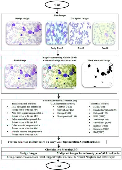
Figure 3.
An outline of the suggested methodology.
3.1. Image Preprocessing Module (IPM)
An important step in making practical, quick, and accurate decisions for identifying cases of acute lymphoblastic leukemia is data preprocessing. The preprocessing process has been done via enhancement contrast with adaptive threshold. The image quality is critical for feature identification and the precision of subsequent measurement. This phase is also known as image enhancement because the image was obtained by improving the contrast and removing errors to achieve a higher quality image for future processes. Images may contain noise or artifacts such as scratches, lapping tracks, comet tails, and so on, which must be removed before proceeding with the processing. The image’s edges and contrast should be improved for greater accuracy and clarity. The image’s colormap was used to improve the image’s boundary and contrast. After obtaining the set of boundary pixels, the updated threshold was calculated as the average of the boundary pixels from the contrasted image [13,14].
3.2. Feature Extraction Module (FEM)
The image’s edges and contrast should be improved for greater accuracy and clarity, and this can be achieved by using the image’s colormap. After obtaining the set of boundary pixels, the updated threshold was calculated by taking the average of the boundary pixels from the contrasted image. The transformation was accomplished through a series of steps depicted in Figure 4.

Figure 4.
Series of transformation steps.
The transformation process can be described as:
Convert the RGB (Red, Green, and Blue) color space to the HSV (Hue, Saturation, and Value) color space; the following formulas were used [15,16].
A color histogram, in general, is based on a specific color space, such as RGB or HSV. The correlogram is obtained when the pixels in an image that contains different colors are calculated. A correlogram can be represented as a table indexed by pairs of colors (i,j), with the dth entry indicating the probability of finding a pixel (j) from pixel (i) at distance d. On the other hand, an auto-correlogram has been stored as a table indexed by color (i), where the dth entry shows the probability of finding pixel (i) from the same pixel at a distance of (d). As a result, the auto-correlogram shows only the spatial correlation between identical colors. Experimental results showed that correlograms and auto-correlograms are both computationally expensive. As a result, a correlogram with a small number of colors and a small distance value will produce very good results without raising the computational cost. Let [D] denote a set of D fixed distances {d1, …, dD}. Then the correlogram of the image (I) has been defined for color pair (ci, cj) at a distance d [16].
The auto-correlogram of the image (I) is defined for color Ci at a distance d.
The color moments were used to differentiate images based on their color characteristics. These moments provide a measure of color similarity between images. These similarity values can be compared with the values of images stored in a database for image retrieval tasks. Color moments are based on the assumption that the color distribution in an image is interpreted as a probability distribution; the number of distinct moments are characterized by the probability distributions. As a result, if the color in an image follows a specific probability distribution, the moments of that distribution can be used as features to identify that image based on color [17].
In general, the image has three central moments of color distribution. They can be expressed as the mean, the standard deviation, and the skewness. A color is defined by three or more values; in the proposed methodology, it can be expressed as the HSV scheme of hue, saturation, and brightness. Therefore, the image is defined by nine moments, three moments for each of the three color channels. The ith color channel at the jth image pixel is denoted as pij. The average color value in the image is represented by the mean (E), the standard deviation (σ) which is the square root of the distribution’s variance, and skewness (S) which is a metric for deciding the level of asymmetry in distribution [17,18].
The channels were represented by a bank of two-dimensional Gabor filters. A two-dimensional Gabor function is made up of a sinusoidal plane wave with some frequencies and orientations that are modulated by a two-dimensional Gaussian envelope. In the spatial domain, the ‘canonical’ Gabor filter is given by [19]:
where ϕ is the phase of the sinusoidal plane wave along the z-axis, and σx is the space constants of the Gaussian envelope along the z-axis. A Gabor filter with arbitrary orientation, θ0, was obtained via a rigid rotation of the x–y coordinate system. These two-dimensional functions were shown to be good fits for the receptive field profiles of simple cells in the striate cortex. A Gabor filter’s frequency and orientation-selective properties are more explicit in its frequency domain representation. The Fourier domain representation specifies how much each frequency component of the input image is modified or modulated by the filter. As a result, such representations are known as modulation transfer functions (MTF) [20].
The following step is to perform the discrete wavelet transform for extracting the moments. The discrete wavelet transform provides more information and is more adaptable. It divides data into frequency components or sub-bands. The wavelet has an advantage over Fourier in analyzing physical situations because the sinusoid does not have a fixed duration but instead extends from minus to plus infinity. Most audio signal loses information in the Fourier transform domain [21,22]. A wavelet expansion coefficient is a local and easy-to-understand component. Wavelets are adjustable, adaptable, and intended for use in adaptive systems, whereas the Fourier transform is appropriate when the signal contains only a few stationary components [22]. There are two types of features as shown in Figure 5.
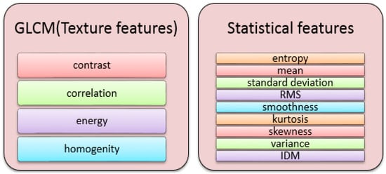
Figure 5.
Features Type.
Texture provides statistics on the spatial arrangement of intensities in an image. Leukemia causes significant changes in the chromatin distribution of WBC nuclei, which can be visualized as texture. Changes in chromatin distribution reflect the organization of DNA in the nucleus and are an important diagnostic descriptor for distinguishing benign from malignant cells.
The texture feature descriptor grey level co-occurrence matrix (GLCM) was used to determine the shape and texture parameters of a nucleus. Second-order statistics, such as the probability of two pixels having specific grey levels at specific spatial relationships, was used to describe grey-level pixel distribution. These data can be represented in 2-dimensional grey level co-occurrence matrices, which can be computed for different distances and orientations. Statistical measures that have been used to extract textual characteristics from the GLCM have been defined. Some of these characteristics are as follows [23,24]:
- 1
- Energy: a measure of image homogeneity.
- 2
- Contrast: a different moment of the regional co-occurrence matrix that measures the contrast or the number of local variations in an image.
- 3
- Correlation: a measure of the image’s regional pattern liner dependencies.
- 4
- Homogeneity: returns a value indicating how close the distribution of elements in the GLCM is to the diagonal GLCM.
In addition to the GLCM features, the statistical features can be described as [24,25,26]:
- 5
- Entropy: the measure of randomness or disorder in the images.
- 6
- Mean: measure of the image’s brightness by calculating the average value of pixels inside the region of interest.
- 7
- Standard deviation: used for deciding what is normal, extra-large, or extra-small.
- 8
- RMS: the root mean square.
- 9
- Smoothness: a measurement of grey level disparity that can be used to create relative smoothness recipes.
- 10
- Kurtosis: measure of the peak of the distribution of the intensity values around the mean.
- 11
- Skewness: assesses the absence of symmetry. The zero value shows that the intensity value distribution is moderately fair to both sides of the mean.
- 12
- Variance: average of squared differences from mean.
- 13
- IDM: measure homogeneity, used with grey image, measure grey level linear dependency of an image
3.3. Feature Selection Module (FSM)
Most high-dimensional datasets contain redundant, noisy, and unimportant features. To enhance classification performance and cut down on operational costs, feature selection aims to reduce the dimensionality of the data and choose only the most crucial features. Finding the best feature is the challenge, especially in the case of vast search space. Finding the fewest and most crucial features that provide enough details to describe the system is the aim of feature selection. In general, feature selection can save processing time, make data interpretation easier, prevent dimensionality affliction, and reduce overfitting. Once a good feature selection is met, the misleading, irrelevant, and redundant features are deleted, resulting in a well-produced feature selection [27,28].
3.3.1. Grey Wolf Optimization Algorithm
The grey wolf optimization algorithm is a straightforward optimization algorithm that draws inspiration from nature and uses its leadership structure to find the ideal answer to a given problem [29,30,31]. Figure 6 depicts the grey wolves’ social (or leadership) structure. It consists of four adjusting parameters as:
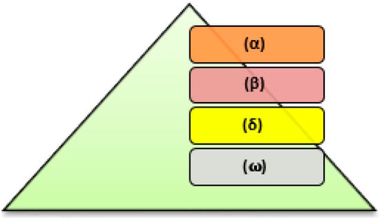
Figure 6.
Hierarchy of grey wolves.
- 1
- Alpha wolves (α) are the hunters’ leaders that make the hunting decisions. They are the pack’s most dominant wolves because their actions are determined and must be followed by the rest of the pack. The alphas do not have to be the strongest members of the pack, but they must be the best at managing the entire pack.
- 2
- Beta wolves (β) occupy the second position in the hierarchy. A beta wolf advises the alpha, assisting those in deciding. If the alpha wolf dies or becomes old, the beta wolf takes his place. Their responsibility is to reinforce the pack’s alpha’s commands and to maintain discipline as one of the levels that are lower in the structure.
- 3
- Omega wolves (ω) occupy the lowest level of the hierarchy and serve as a scapegoat. They should surrender to the dominant wolves in the structure, and they should eat last.
- 4
- Delta wolf (δ), a wolf who is neither an alpha, beta, nor omega, is known as a subordinate wolf in the pack. Delta wolves report to alphas or betas, but they have authority over omega wolves [32].
3.3.2. Grey Wolf Optimization Mathematical Modeling
Using a set of random positions, each of which is stored in a vector, the grey wolf optimization algorithm can begin the optimization process. The first step of each repetition begins with computing the alpha, beta, and delta wolves’ fitness values. To keep track of the wolves’ locations and fitness values, three vectors and three variables are used. Before the location updating process can begin, first alpha, beta, and delta wolves’ locations must be updated. According to the updated wolf location, the distance between the three wolves/agents and the current solution must be measured. This is illustrated in Figure 7.
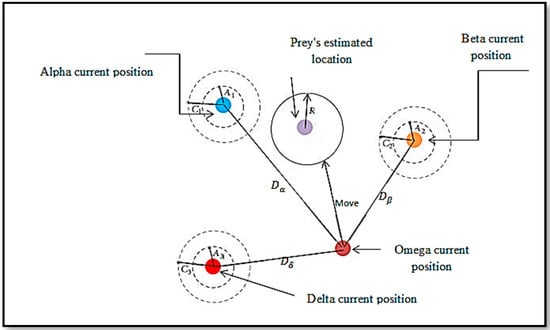
Figure 7.
Updating the Grey wolf’s position.
The three best locations for the wolves are used to determine the new locations for the wolves, as shown in equations below [33,34,35].
where , , are defined as:
The variables,, , and represent three best positions at iteration t, ,,, and ,, are the coefficient vectors, which are computed as follows:
where will linearly decrease from 2 to 0 over the course of iterations, and are the random vectors in [0, 1]. The equation for updating the () the parameter is given by:
In the grey wolf optimization algorithm, the global search (exploration) occurs when A < 1 or A > 1, whereas the local search (exploitation) occurs when 1 > A > −1. The A value is determined by the (a) parameter, which decreases linearly from 2 to 0. The variable A’s field changes in the range [−2, 2] as a result of the random mechanisms in this variable. Overall, as previously stated, balancing exploitation and exploration is required to achieve the global optimum using a stochastic method [31]. Finally, the flowchart details of the grey wolf optimization algorithm is illustrated in Figure 8.
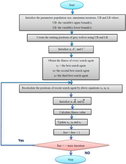
Figure 8.
Flowchart of the grey wolf optimization algorithm.
3.4. Classification Module (CM)
The proposed approach uses four different types of classifiers: support vector machine, random forest, k-nearest neighbor, and naïve Bayes [36,37]. This section discusses the classification techniques in brief.
3.4.1. Support Vector Machine (SVM)
This machine learning algorithm is very effective. Compared with other machine learning algorithms, it has several benefits. For classifying space, it offers the best decision boundary. The decision boundary, as depicted in Figure 9, acts as a boundary between various classes of points. It also has the biggest margin, and because they help and support the algorithm, the points on the margin are known as support vectors. The maximum margin hyperplane or maximum margin classifier refers to the line of the decision boundary, which is located in the middle of the margin [38].
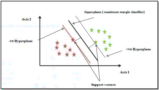
Figure 9.
Hyper-plane separation between two datasets.
3.4.2. Random Forest (RF)
This algorithm generates a collection of techniques that function as a whole and is described as a decision tree forest made up entirely of random and various tree-loaded techniques. It is chosen by the majority after being measured from multiple decision trees. It is thought to be one of the most effective algorithms. Although it performs well in both classification and regression, overfitting is the main drawback of this approach [39].
3.4.3. K-Nearest Neighbor (KNN)
In statistical prediction techniques and pattern recognition, the supervised k-nearest neighbor algorithm is employed. According to Figure 10, this algorithm’s classification goal is based on the majority of its neighbors. In this model space, the number of neighbors close to the test point is denoted by the positive integer k. The magnitude of k has an impact on the KNN algorithm’s accuracy because a high value of k reduces the impact of noise on classification and increases algorithm accuracy [39].
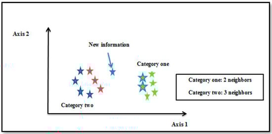
Figure 10.
K-Nearest Neighbor example.
3.4.4. Naïve Bayes (NB)
To classify new objects, Bayesian classifiers assign membership probabilities. It is a fast method and can produce reasonably good results, even when applied to large amounts of data. The two Bayesian classifiers can be divided into naïve Bayes and Bayesian networks. The naïve Bayes classifier represents the learning probabilistic knowledge of the Bayes theorem using a simple approach with clear semantics. It assumes, in particular, that the predictive attributes are conditionally independent given the class, and it demonstrates that there are no hidden or latent attributes that can influence the prediction process. An investigation was conducted to evaluate the performance of the machine learning tool. The naïve Bayes classifier, on the other hand, can be used to classify ALL leukemia. Furthermore, in the field of medical data mining, it can be used in enhancing the accuracy of ALL detection [40,41].
4. Results
4.1. The Demographic Characteristics:
The working dataset included 504 PBS images for 25 healthy people with a benign diagnosis and 2685 images for 64 patients that have been diagnosed as malignant with ALL subtypes. The demographic characteristics are described in Table 2. The proposed framework for the leukemia diagnosis is illustrated in Figure 11 and are listed as:
Table 2.
The Demographic characteristics.
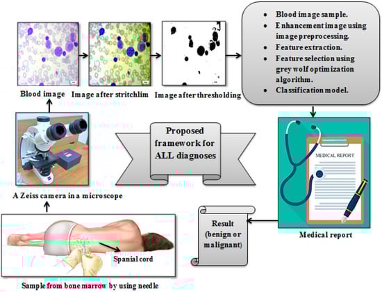
Figure 11.
Proposed framework for leukemia diagnosis.
- A
- The image was enhanced by using stretchlim and adaptive thresholing.
- B
- Extracting features was carried out by using feature extraction methods.
- C
- The number of features was reduced by using the grey wolf optimization technique.
- D
- Acute lymphoblastic leukemia was classified into benign and malignant using RF, SVM, KNN, and NB classifiers.
4.2. Performance Measures
Various classification algorithms such as random forest, support vector machine, k-nearest neighbor, and naïve Bayes have been used in the classification of ALL. To ensure the effectiveness of the proposed methodology, several performance metrics [14,42] have been calculated to perform a fair comparison between the classifiers and the influence of using the grey wolf optimization algorithm as a feature selection algorithm.
These performance metrics are illustrated in Table 3. The evaluated metrics include accuracy, precision, recall (the most important one), F1-score, and specificity [43], which is required for evaluating binary classification.
Table 3.
Equations for confusion matrices with descriptions.
These evaluation metrics indicators require the following parameters to be calculated:
- “TP” (true positives): the number of infected cases expected to be infected.
- “TN” (true negatives): the number of uninfected cases expected to be uninfected.
- “FP” (false positives): the number of uninfected cases expected to be infected.
- “FN” (false negatives): the number of infected cases expected to be uninfected.
- Note: In the proposed methodology the patient represents a positive class (0 is benign, 1 is malignant).
The classification results before using the grey wolf optimization algorithm with all 203 features are shown in Table 4 and Figure 12.
Table 4.
The performance metrics for different classification techniques before using grey wolf optimization algorithm.
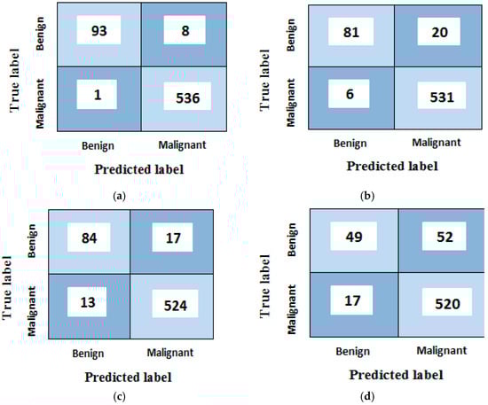
Figure 12.
Confusion matrices analyses of the proposed model for (a) random forest, (b) support vector machine, (c) k-nearest neighbor and (d) naïve Bayes classifiers before using grey wolf optimization algorithm.
Figure 12a shows that (93) images are correctly recognized, whereas (8) benign samples are recognized as malignant type (false positive). It also discloses that (536) malignant samples are rightly classified, whereas only (1) samples are improperly classified as benign type (false negative). Corresponding results are found for the rest of the confusion matrices b, c, and d.
The classification results after using the grey wolf optimization algorithm are shown in Table 5 and Figure 13.
Table 5.
The performance metrics for different classification techniques after using grey wolf optimization algorithm.
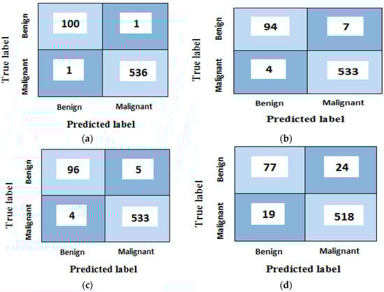
Figure 13.
Confusion matrices analyses of the proposed model for (a) random forest, (b) support vector machine, (c) k-nearest neighbor and (d) naïve Bayes classifiers after using grey wolf optimization algorithm.
Figure 13a shows that (100) images have been correctly classified, whereas (1) benign samples are recognized as malignant type (false positive). It also discloses that (536) malignant samples have been correctly classified, whereas only (1) samples are improperly classified as benign type (false negative). Corresponding results are found for the rest of the confusion matrices b, c, and d. Figure 14 shows the confusion matrices for all classes before and after using the grey wolf optimization algorithm.
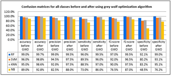
Figure 14.
Confusion matrices before and after using grey wolf optimization algorithm.
As shown in Figure 14, ALL detection before using the grey wolf optimization algorithm was able to achieve an average sensitivity of 96%, specificity of 92.1%, accuracy of 99%, F1-score of 97%, and precision of 99% when applying RF. In addition, it was able to achieve an average sensitivity of 89.5%, specificity of 80.2%, accuracy of 96%, F1-score of 92%, and precision of 94.5% when applying the SVM classifier. We were able to obtain an average sensitivity of 88.5%, specificity of 83.2%, accuracy of 95%, F1-score of 90%, and precision of 92% when applying the KNN classifier. When we applied the NB classifier, we reached an average sensitivity of 73%, specificity of 48.5%, the accuracy of 89%, F1-score of 76.5%, and precision of 82.5%.
After using the grey wolf optimization algorithm as a feature-selection algorithm for enhancing the classification techniques, the accuracy of the classification techniques was improved, as was sensitivity, precision, F1-score, and specificity.
For ALL detection after using the grey wolf optimization algorithm, it was able to achieve an average sensitivity of 99.5%, specificity of 99%, accuracy of 99.7%, F1-score of 99.5%, and precision of 99.5% when applying the RF classifier. In addition, it was able to achieve an average sensitivity of 96%, specificity of 93.1%, the accuracy of 98.8%, F1-score of 96.5%, and precision of 97.5% when applying the SVM classifier. We were able to obtain an average sensitivity of 97%, specificity of 95.1%, the accuracy of 98.6%, F1-score of 97.5%, and precision of 97.5% when applying the KNN classifier. When the NB classifier was applied, we achieved average sensitivity of 86%, specificity of 76.2%, the accuracy of 92.8%, F1-score of 87%, and precision of 88%. Figure 15 shows the effect of using grey wolf in feature selection on the confusion matrices.
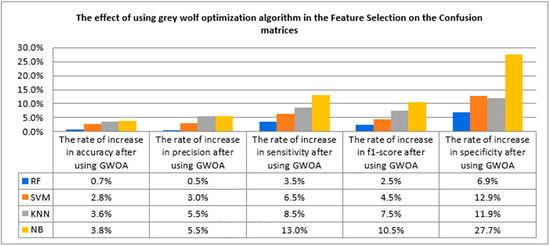
Figure 15.
The rate of increase in confusion matrices after using grey wolf optimization algorithm.
After using the grey wolf algorithm in features selection, it was found that the rate of increase in accuracy became 0.7% in RF, 2.8% in SVM, 3.6% in KNN, and 3.8% in NB. The rate of increase in precision became 0.5% after using RF, 3%, 5.5%, and 5.5% after using SVM, KNN, and NB, respectively. Sensitivity also increased after using the grey wolf technique and became 3.5%, 6.5%, 8.5%, and 13% of RF, SVM, KNN, and NB, respectively. The rate of increase in specificity became 6.9%, 12.9%, 11.9%, and 27.7% when using RF, SVM, KNN, and NB, respectively.
The grey wolf optimization algorithm reduced the number of features while achieving the highest performance, which facilitates the process of detecting whether the blood sample is benign or malignant as shown in Figure 16.
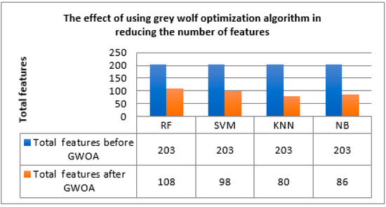
Figure 16.
Effect of grey wolf in reducing the number of features.
5. Comparative Results
A comparative result between the proposed and the other techniques in the literature was performed. Additionally, we compared machine learning algorithms SVM, NB, KNN, and RF algorithms for the binary classification. Table 6 shows different study results.
Table 6.
Performance comparison of the proposed method and other machine learning classifiers.
Sorayya et al. [1] attempted to investigate deep CNN applications in which they developed pre-trained VGG-16 and ResNet for the diagnosis and classification of ALL and identified between healthy and cancer cases. They were able to achieve 81.6% ResNet, 84.6% VGG-16, 77.9% KNN, and 82.1% proposed CNN testing accuracy. These classifiers measured the overall precision, sensitivity, and F1-score, which are summarized in Table 6. The highest precision of 85% was obtained with VGG-16, the highest sensitivity of 83.5% with VGG-16, and the highest F1-score of 84% with VGG-16. While the proposed work was superior to that of Sorayya et al. [1], it achieved the highest accuracy when a random forest classifier was used. It reached 99.7% accuracy in correctly classifying acute lymphoblastic leukemia cases based on the total number of test images. The precision, which measures the number of correct positive classes, was 99.5%. The model had a specificity of 99% when comparing the true proportion of negative results with all actual negatives. The F1-score obtained indicates that the model was effective at identifying benign cases; it was 99.5%. When the proportion of true positives to all actual positives was calculated by the RF classifier, recall reached 99.5%.
Amirarash et al. [2] sought to classify treatment outcomes for 241 ALL children and adolescents aged three months to seventeen at the time of diagnosis. Amirarash et al. [2] used SVM with a cost parameter of 100 and outperformed it with an accuracy of 94.9%, precision of 90.2%, sensitivity of 86.2%, and F1-measure of 88.2%. They also used the RF classifier, which had an accuracy of 90.9%, a precision of 79.6%, a sensitivity of 92.2%, and an F1-measure of 85.4%. While the proposed work outperformed that of Amirarash et al. [2], it achieved the highest accuracy when using a random forest classifier. This means that it reached 99.7% accuracy when calculating accuracy by dividing the number of correctly classified acute lymphoblastic leukemia cases by the total number of test images. The precision, which measures the number of correct positive classes, was 99.5%. The model had a specificity of 99% when comparing the true proportion of negative results to all actual negatives. The F1-score obtained indicates that the model was effective at identifying benign cases; it was 99.5%. When the proportion of true positives to all actual positives was calculated by the RF classifier, recall reached 99.5%. With an overall accuracy of 98.8%, the proposed model employed an SVM classifier that outperformed that used by Amirarash et al. [2]. The accuracy was 98.8%. When the SVM classifier was used to calculate the true positive rate, sensitivity reached 96%. The obtained F1-score was 96.5%. The model had a specificity of 93.1% when measuring the true negative rate.
Sarmad et al. [4] made use of the Public ALL-IDB 1 (108 images). The highest accuracy achieved by this study when using SVM was 93.7%. The proposed work outperformed Sarmad et al. [4]; the proposed model employed an SVM classifier that outperforms the one used in [4] with overall correctness of 98.8% which means the classifier’s ability to correctly classify the class label was higher than that of Sarmad et al. [4].
Payam et al.’s [7] proposed approach was able to fuse features extracted from the best deep learning models and outperformed individual networks with an accuracy of 96.6%, precision of 96.9%, sensitivity of 91.75%, and F1-score of 94.7% in Leukemic B-lymphoblast diagnosis. When comparing these results with our proposed methodology, we found that the results of our suggestions when using RF were higher in accuracy, sensitivity, and specificity as shown in Table 6.
Sara et al. [9] presented an automatic CNN hybrid method for the classification of ALL and healthy cells with an accuracy of 96.2%, sensitivity of 95.2%, and specificity of 98.6%. When comparing these results with our proposed methodology, we found that the results of our suggestions when using RF were higher in accuracy, sensitivity, and specificity as shown in Table 6.
The ALL-DB dataset was used by Nizar et al. [10]. When the classifier CNN was used in this study, the highest accuracy was 88.3%. The accuracy achieved by this study was 50.1% when using SVM and 69.7% when using NB. The proposed model employed an SVM classifier that was superior to that used by Nizar et al. [10], with an overall accuracy of 98.8%; additionally, the proposed model employed an NB classifier with an overall accuracy of 92.8%, which means the classifier’s ability to correctly classify the class label was higher than that of Nizar et al. [10].
S. Alagu et al. [11] proposed work to suggest principal features for the detection of ALL. The highest accuracy achieved by this study when using (AlexNet+GoogleNet+SqueezeNet+SVM) was 98.2%, precision of 99.2%, recall of 98.1%, F1-score of 96.3%, and specificity of 99.1%. This means that S. Alagu et al.’s [11] proposed work had the ability to correctly identify people who did not have the disease by 0.1% from our proposed methodology. However, compared with the proposed methodology, it was found that the accuracy is increased by 1.5%, which means that the classifier’s ability to correctly classify the naming of the class was higher. Moreover, it had a higher number of correct positive categories with a percentage of 0.3% and was higher in calculating the number of correct positive classes made out of all positive classes classification with a percentage of 1.4%.
Figure 17 shows a comparison between the accuracy generated when using the classifiers after applying a grey wolf for feature selection. From the results, it is clear that the proposed methodology can achieve the highest accuracy over the rest of the classifiers used in the other references, as exhibited in Table 6. This clearly illustrates that all the values of the confusion matrices resulting from the proposed work are higher than all the values obtained from the methods used in the references that are presented in Table 6.
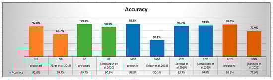
Figure 17.
A graph showing classifiers’ accuracy obtained from the proposed work and the similar classifiers used in other references [1,2,4,10].
6. Conclusions
The detection of immature leukemic blasts and normal cells is one of the great interests for saving human life, especially those who suffer from blood cancer. Attempts were made in this research to detect acute lymphoblastic leukemia from microscopic blood images using image processing techniques. The dataset used included 3189 PBS images from 89 patients suspected of having ALL, whose blood samples were organized and stained by highly skilled laboratory personnel. This dataset was split into two categories: benign and malignant. Firstly, the image was enhanced by using stretchlim and adaptive thresholding. Secondly, extracting features was carried out by using feature extraction methods. Thirdly, the number of features was reduced by using the grey wolf optimization algorithm. Finally, acute lymphoblastic leukemia was classified into benign and malignant using RF, SVM, KNN, and naïve Bayes classifiers. After employing the grey wolf optimization technique in the feature selection process, it was demonstrated that it provides good efficiency in all cases. The proposed work obtained the highest accuracy of 99.69%, the highest sensitivity of 99.5%, the highest precision of 99.5%, F1-score of 99.5%, and specificity of 99%, proving the efficacy of these methods. These methods were compared to some modern techniques to determine the efficacy of the suggested method.
Compared with previous research, it was found that the highest accuracy resulted from the proposed methodology. Thus, the proposed proposal can improve performance and reduce the number of features after using the grey wolf optimization technique, this is the first time that grey wolf has been used in detecting ALL leukemia. Furthermore, using other approaches for this methodology is of interest to use more effective approaches in the next research for more improved results.
Author Contributions
N.M.S.: writing the paper, image preprocessing, feature selection, and A.I.S. code for machine learning technique. H.A.A.: feature extraction and paper editing. M.M.A.: AI classification techniques, designing the study, editing the paper, and review. N.M.S. and M.M.A. contributed to research idea development, data collection, and data analysis. All authors contributed to the drafting of the manuscript, and M.M.A. revised the manuscript. All authors have read and agreed to the published version of the manuscript.
Funding
This research received no external funding.
Institutional Review Board Statement
The study did not require ethical approval.
Informed Consent Statement
Informed consent was obtained from all subjects involved in the study according to the dataset owner.
Data Availability Statement
Data is available on a reasonable request.
Acknowledgments
The authors would like to express appreciation to Mansoura University for supporting the authors.
Conflicts of Interest
The authors declare no conflict of interest.
References
- Rezayi, S.; Mohammadzadeh, N.; Bouraghi, H.; Saeedi, S.; Mohammadpour, A. Timely Diagnosis of Acute Lymphoblastic Leukemia Using Artificial Intelligence-Oriented Deep Learning Methods. Comput. Intell. Neurosci. 2021, 2021, 5478157. [Google Scholar] [CrossRef] [PubMed]
- Kashef, A.; Khatibi, T.; Mehrvar, A. Treatment outcome classification of pediatric Acute Lymphoblastic Leukemia patients with clinical and medical data using machine learning: A case study at MAHAK hospital. Inform. Med. Unlocked 2020, 20, 100399. [Google Scholar] [CrossRef]
- Mondal, C.; Hasan, M.; Jawad, M.; Dutta, A.; Islam, M.; Awal, M.; Ahmad, M. Acute Lymphoblastic Leukemia Detection from Microscopic Images Using Weighted Ensemble of Convolutional Neural Networks. arXiv 2021, arXiv:2105.03995. [Google Scholar]
- Shafique, S.; Tehsin, S.; Anas, S.; Masud, F. Computer-assisted Acute Lymphoblastic Leukemia detection and diagnosis. In Proceedings of the 2019 2nd International Conference on Communication, Computing and Digital systems (C-CODE), Islamabad, Pakistan, 6–7 March 2019; pp. 184–189. [Google Scholar] [CrossRef]
- Ghaderzadeh, M.; Aria, M.; Hosseini, A.; Asadi, F.; Bashash, D.; Abolghasemi, H. A fast and efficient CNN model for B-ALL diagnosis and its subtypes classification using peripheral blood smear images. Int. J. Intell. Syst. 2021, 37, 5113–5133. [Google Scholar] [CrossRef]
- Aftab, M.O.; Awan, M.J.; Khalid, S.; Javed, R.; Shabir, H. Executing Spark BigDL for Leukemia Detection from Microscopic Images using Transfer Learning. In Proceedings of the 2021 1st International Conference on Artificial Intelligence and Data Analytics (CAIDA), Riyadh, Saudi Arabia, 6–7 April 2021; pp. 216–220. [Google Scholar]
- Kasani, P.H.; Park, S.-W.; Jang, J.-W. An Aggregated-Based Deep Learning Method for Leukemic B-lymphoblast Classification. Diagnostics 2020, 10, 1064. [Google Scholar] [CrossRef]
- Sahlol, A.T.; Kollmannsberger, P.; Ewees, A.A. Efficient Classification of White Blood Cell Leukemia with Improved Swarm Optimization of Deep Features. Sci. Rep. 2020, 10, 2536. [Google Scholar] [CrossRef]
- Kassani, S.H.; Kassani, P.H.; Wesolowski, M.J.; Schneider, K.A.; Deters, R. A hybrid deep learning architecture for leukemic B-lymphoblast classification. In Proceedings of the 2019 International Conference on Information and Communication Technology Convergence (ICTC), Jeju Island, Korea, 16–18 October 2019; pp. 271–276. [Google Scholar]
- Ahmed, N.; Yigit, A.; Isik, Z.; Alpkocak, A. Identification of Leukemia Subtypes from Microscopic Images Using Convolutional Neural Network. Diagnostics 2019, 9, 104. [Google Scholar] [CrossRef]
- Alagu, S. Automatic Detection of Acute Lymphoblastic Leukemia Using UNET Based Segmentation and Statistical Analysis of Fused Deep Features. Appl. Artif. Intell. 2021, 35, 1952–1969. [Google Scholar] [CrossRef]
- Kumar, D.; Jain, N.; Khurana, A.; Mittal, S.; Satapathy, S.C.; Senkerik, R.; Hemanth, J.D. Automatic Detection of White Blood Cancer from Bone Marrow Microscopic Images Using Convolutional Neural Networks. IEEE Access 2020, 8, 142521–142531. [Google Scholar] [CrossRef]
- Rawat, J.; Singh, A.; Bhadauria, H.S.; Virmani, J.; Devgun, J.S. Classification of acute lymphoblastic leukaemia using hybrid hierarchical classifiers. Multimedia Tools Appl. 2017, 76, 19057–19085. [Google Scholar] [CrossRef]
- Sarki, R.; Ahmed, K.; Wang, H.; Zhang, Y.; Ma, J.; Wang, K. Image Preprocessing in Classification and Identification of Diabetic Eye Diseases. Data Sci. Eng. 2021, 6, 455–471. [Google Scholar] [CrossRef]
- Shereena, V.B.; David, J.M. Content Based Image Retrieval: A Review. Comput. Sci. Inf. Technol. 2014, 65–77. [Google Scholar] [CrossRef]
- Ojala, T.; Rautiainen, M.; Matinmikko, E.; Aittola, M. Semantic image retrieval with HSV correlograms. In Proceedings of the Scandinavian conference on Image Analysis, Bergen, Norway, 11–14 June 2001; pp. 621–627. [Google Scholar]
- Tigistu, T.; Abebe, G. Classification of rose flowers based on Fourier descriptors and color moments. Multimedia Tools Appl. 2021, 80, 36143–36157. [Google Scholar] [CrossRef]
- Damayanti, F.; Muntasa, A.; Herawati, S.; Yusuf, M.; Rachmad, A. Identification of Madura Tobacco Leaf Disease Using Gray-Level Co-Occurrence Matrix, Color Moments and Naïve Bayes. J. Phys. Conf. Ser. 2020, 1477, 052054. [Google Scholar] [CrossRef]
- Singh, R.; Goel, A.; Raghuvanshi, D.K. Computer-aided diagnostic network for brain tumor classification employing modulated Gabor filter banks. Vis. Comput. 2021, 37, 2157–2171. [Google Scholar] [CrossRef]
- Sultan, S.; Ghanim, M.F. Human Retina Based Identification System Using Gabor Filters and GDA Technique. J. Commun. Softw. Syst. 2020, 16, 243–253. [Google Scholar] [CrossRef]
- Starosolski, R. Hybrid Adaptive Lossless Image Compression Based on Discrete Wavelet Transform. Entropy 2020, 22, 751. [Google Scholar] [CrossRef] [PubMed]
- Osadchiy, A.; Kamenev, A.; Saharov, V.; Chernyi, S. Signal Processing Algorithm Based on Discrete Wavelet Transform. Designs 2021, 5, 41. [Google Scholar] [CrossRef]
- Iqbal, N.; Mumtaz, R.; Shafi, U.; Zaidi, S.M.H. Gray level co-occurrence matrix (GLCM) texture based crop classi-fication using low altitude remote sensing platforms. PeerJ Comput. Sci. 2021, 7, e536. [Google Scholar] [CrossRef]
- Albregtsen, F. Statistical Texture Measures Computed from Gray Level Coocurrence Matrices; Image Processing Laboratory, Department of Informatics, University of Oslo: Oslo, Norway, 2008; Volume 5. [Google Scholar]
- Hariprasath, S.; Dharani, T.; Santhi, M. Detection of acute lymphocytic leukemia using statistical features. In Proceedings of the 4th International Conference on Current Research in Engineering Science and Technology, Tamil Nadu, India, 8 March 2019. [Google Scholar]
- Mutlag, W.K.; Ali, S.K.; Aydam, Z.M.; Taher, B.H. Feature Extraction Methods: A Review. J. Phys. Conf. Ser. 2020, 1591, 012028. [Google Scholar] [CrossRef]
- Al-Tashi, Q.; Rais, H.; Abdulkadir, S.J.; Mirjalili, S.; Alhussian, H. A Review of Grey Wolf Optimizer-Based Feature Selection Methods for Classification. In Evolutionary Machine Learning Techniques. Algorithms for Intelligent Systems; Mirjalili, S., Faris, H., Aljarah, I., Eds.; Springer: Singapore, 2020; pp. 273–286. [Google Scholar] [CrossRef]
- Abdollahzadeh, B.; Gharehchopogh, F.S. A multi-objective optimization algorithm for feature selection problems. Eng. Comput. 2021, 38, 1845–1863. [Google Scholar] [CrossRef]
- Hu, P.; Pan, J.-S.; Chu, S.-C. Improved Binary Grey Wolf Optimizer and Its application for feature selection. Knowl.-Based Syst. 2020, 195, 105746. [Google Scholar] [CrossRef]
- Hu, P.; Pan, J.-S.; Chu, S.-C.; Chai, Q.-W.; Liu, T.; Li, Z.-C. New Hybrid Algorithms for Prediction of Daily Load of Power Network. Appl. Sci. 2019, 9, 4514. [Google Scholar] [CrossRef]
- Raj, S.; Bhattacharyya, B. Optimal placement of TCSC and SVC for reactive power planning using Whale optimization algorithm. Swarm Evol. Comput. 2018, 40, 131–143. [Google Scholar] [CrossRef]
- Kumar, S.; Singh, M. Breast Cancer Detection Based on Feature Selection Using Enhanced Grey Wolf Optimizer and Support Vector Machine Algorithms. Viet. J. Comput. Sci. 2021, 8, 177–197. [Google Scholar] [CrossRef]
- Almazini, H.; Ku-Mahamud, K.R. Grey Wolf Optimization Parameter Control for Feature Selection in Anomaly Detection. Int. J. Intell. Eng. Syst. 2021, 14, 474–483. [Google Scholar] [CrossRef]
- Chawla, V.; Chanda, A.K.; Angra, S. The scheduling of automatic guided vehicles for the workload balancing and travel time minimi-zation in the flexible manufacturing system by the nature-inspired algorithm. J. Proj. Manag. 2019, 4, 19–30. [Google Scholar] [CrossRef]
- Kitonyi, P.M.; Segera, D.R. Hybrid Gradient Descent Grey Wolf Optimizer for Optimal Feature Selection. BioMed Res. Int. 2021, 2021, 2555622. [Google Scholar] [CrossRef]
- Shiva, C.K.; Gudadappanavar, S.S.; Vedik, B.; Babu, R.; Raj, S.; Bhattacharyya, B. Fuzzy-Based Shunt VAR Source Placement and Sizing by Oppositional Crow Search Algorithm. J. Control. Autom. Electr. Syst. 2022, 33, 1576–1591. [Google Scholar] [CrossRef]
- Shekarappa, G.S.; Mahapatra, S.; Raj, S. Voltage constrained reactive power planning problem for reactive loading variation using hybrid harris hawk particle swarm optimizer. Electr. Power Compon. Syst. 2021, 49, 421–435. [Google Scholar] [CrossRef]
- Balaraman, S. Comparison of Classification Models for Breast Cancer Identification using Google Colab. Preprints 2020, 2020050328. [Google Scholar] [CrossRef]
- Sanlı, T.; Sıcakyüz, Ç.; Yüregir, O.H. Comparison of the accuracy of classification algorithms on three data-sets in data mining: Example of 20 classes. Int. J. Eng. Sci. Technol. 2020, 12, 81–89. [Google Scholar] [CrossRef]
- Amancio, D.R.; Comin, C.; Casanova, D.; Travieso, G.; Bruno, O.; Rodrigues, F.; Costa, L.D.F. A Systematic Comparison of Supervised Classifiers. PLoS ONE 2014, 9, e94137. [Google Scholar] [CrossRef]
- Bafjaish, S.S. Comparative Analysis of Naive Bayesian Techniques in Health-Related for Classification Task. J. Soft Comput. Data Min. 2020, 1, 1–10. [Google Scholar]
- Bibi, N.; Sikandar, M.; Ud Din, I.; Almogren, A.; Ali, S. IoMT-based automated detection and classification of leukemia using deep learning. J. Healthc. Eng. 2020, 2020, 6648574. [Google Scholar] [CrossRef] [PubMed]
- Jiang, Z.; Dong, Z.; Wang, L.; Jiang, W. Method for Diagnosis of Acute Lymphoblastic Leukemia Based on ViT-CNN Ensemble Model. Comput. Intell. Neurosci. 2021, 2021, 7529893. [Google Scholar] [CrossRef]
Publisher’s Note: MDPI stays neutral with regard to jurisdictional claims in published maps and institutional affiliations. |
© 2022 by the authors. Licensee MDPI, Basel, Switzerland. This article is an open access article distributed under the terms and conditions of the Creative Commons Attribution (CC BY) license (https://creativecommons.org/licenses/by/4.0/).