Abstract
Although uncertainties such as solar radiation and material properties are generally involved in the solar receiver design process, current studies in the solar receiver field are based on deterministic models and do not incorporate these uncertainties into the design process. In this paper, based on a coupled deterministic thermal–structural model and an uncertainty analysis model, an analysis of temperature and thermal stress was conducted for a solar power tower (SPT) molten salt receiver under multi-source uncertainties to investigate the dispersions of responses. The results demonstrated that the maximum temperature inside the tube wall under multi-source uncertainties ranged from 847 K to 895 K, with an expectation of 871 K and a standard deviation of 8 K, and the maximum thermal stress ranged from 173 MPa to 245 MPa, with an expectation of 204 MPa and a standard deviation of 12 MPa, both of which had severer probabilities than the deterministic results (871 K and 204 MPa) and may cause failure in the receiver. Furthermore, the results of the global sensitivity analysis indicated that the peak incident solar flux was the most sensitive, and the specific heat of the tube material was the least sensitive to the maximum temperature and thermal stress of the tube wall. These results are beneficial to provide additional reliability and confidence in the temperature and thermal stress evaluation process of solar receiver tubes.
1. Introduction
Nowadays, solar energy has attracted extensive attention due to its renewability and low pollution. Among the different concentrated solar technologies, the solar power tower (SPT) system has great potential for development because of its high working temperature and large-scale utilization. The SPT system operates by focusing thousands of heliostats onto a receiver located at the top of a central tower [1]. The receiver is a key part of the SPT system and often undergoes high and nonuniform solar flux radiation, which would easily cause overheating and fatigue damage in the receiver [2,3].
In recent years, many investigations have been conducted on the temperature analysis of the receiver tube wall using the finite volume method (FVM) [4,5,6,7]. Ortega et al. [4] performed CFD modeling with ANSYS Fluent to obtain the temperature distribution of a s-CO2 receiver tube by estimating convection and radiation heat loss. Yang et al. [5] also applied the commercial CFD software Fluent to simulate the heat transfer process of a solar receiver tube. Their results showed that the experimental results were consistent with the numerical results. As a result, the thermal analysis of the receiver tube can be well acquired by the numerical method.
Based on the thermal performance of the receiver tube, the thermal stress analysis of the receiver tube can be performed. Some researchers utilized different theoretical equations to conduct thermal stress analysis [8,9,10,11,12,13,14]. The axial and circumferential temperature gradients are usually neglected by theoretical equations. Therefore, the results obtained by theoretical equations may not be accurate enough when the axial and circumferential temperature gradients cannot be neglected, compared with the radial temperature gradient. To solve this problem, some researchers recently employed the finite element method (FEM) to obtain the thermal stress distribution of the receiver tube wall [15,16,17,18,19]. Peng et al. [15] performed a coupled fluid–thermal–structural analysis to acquire the thermal stress distribution of the SPT receiver. The heat transfer process is numerically simulated with FVM, which is used to calculate the thermal stress. Ortega et al. [16] also obtained the radial, circumferential, and axial stresses throughout the tube by using the ANSYS Structural software based on the temperature distribution solution using ANSYS Fluent.
The studies mentioned above were based on deterministic models with unchanged input parameters. However, uncertainties such as solar radiation and material properties widely exist in the operation process of the receiver, and input parameters should be assigned with probability distributions. For instance, the peak solar flux on the receiver tube wall is a typical uncertain parameter and is generally decided by the level of direct normal irradiance, which is assigned as a normal probability distribution with a square deviation of 5.4% [20,21]. Another important uncertain parameter is the property of the receiver tube wall material, such as absorptance, which is affected by measurement error and performance degradation during long-term use [22]. The receiver tube wall absorptance is assigned as a uniform probability distribution with a range between 0.91 and 0.95 [22,23]. In addition, other input parameters, such as the thermophysical properties of the heat transfer fluid inside the tube, usually deviate from the nominal values [24].
Furthermore, the uncertainties of the input parameters may lead to the dispersions of the temperature and thermal stress inside the receiver tube wall, which may be more severe than the deterministic results. Sánchez-González [8] pointed out that molten nitrate salts become corrosive at higher temperatures of the receiver tube wall and receiver fatigue failure occurs with higher thermal stress in the tube wall. As a result, to guarantee the operation safety of the receiver, it is necessary to determine the dispersions of temperature and thermal stress inside the tube wall by taking the uncertainties into account.
The uncertainty analysis method has been widely used for the safety assessment of engineering structures [25,26,27]. Jiang and Ye [25] calculated the seismic risk of the building in servicing life under various uncertainties. Compared with the case of a deterministic model, the collapse probability of the case under uncertainty increased by 133%. Luo et al. [26] established a hybrid uncertain analysis model of nanobeams to estimate the lower and upper bounds of the response deflection by considering the uncertainties of the materials and loads. Zhou et al. [27] also applied the uncertainty analysis method to accurately quantify the dispersions of the mechanical responses for a fiber-reinforced polymer composite truss bridge with hybrid random and interval uncertainties. Although the uncertainty analysis method has been applied in many areas, its application in the field of solar receivers is rare. Therefore, in this study, the uncertainty analysis method is introduced to obtain the dispersions of temperature and thermal stress inside the tube wall under multi-source uncertainties.
The main objective of this paper is to obtain the lower and upper bounds of the maximum temperature and thermal stress inside an SPT molten salt receiver tube wall under multi-source uncertainties. For that purpose, a deterministic, coupled thermal–structural model of the receiver tube is first demonstrated by importing the inner and outer tube wall temperature distributions from the FVM simulation to the FEM calculation. Then, the uncertain input parameters are identified and assigned with appropriate probability distributions. Furthermore, an uncertainty propagation analysis method is applied to obtain the probability distributions of the maximum temperature and thermal stress inside the receiver tube wall by combining the response surface approximation model and Monte Carlo (MC) simulations. Finally, the importance ranking of uncertainty sources is evaluated by using the global sensitivity analysis method. The results are beneficial to provide additional reliability and confidence in the temperature and thermal stress evaluation process of SPT molten salt receiver tubes.
2. Deterministic Model
2.1. Boundary Conditions
For the SPT molten salt receiver tube, its length and inner/outer radius are 3 m and 10.5/12.5 mm, respectively. The heat transfer fluid is molten nitrate salt (60% NaNO3 + 40%KNO3), and the tube material is 316H stainless steel.
Figure 1 depicts the physical model of the receiver tube. The inlet temperature and inlet velocity of the heat transfer fluid are, respectively, 673 K and 3 m/s. The incident solar flux onto the receiver tube is generally nonuniform and the expression is as follows:
where the peak incident solar flux M = 900 kW/m2 is imposed at the tube crown, and θ and z are described in Figure 1. Only half of the receiver tube is subjected to the high solar flux, which is assumed to have a normal distribution along the axial direction [2,28].
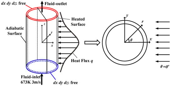
Figure 1.
Physical model of the solar receiver tube.
The heat losses qloss of the receiver tube caused by reflection, convection, and radiation can be calculated as follows [29]:
where α and ε are, respectively, the absorptivity and emissivity of the tube coating material and both taken as 0.93. The convective heat transfer coefficient outside tube wall h is assumed as 10 W/m·K, and the ambient temperature Tamb is 25 °C. Twall is the outer wall temperature of the receiver tube, and σ is the Boltzmann constant.
In addition, Figure 1 shows that there is no constraint at both ends of the receiver tube. Consequently, the thermal stress is caused by the temperature gradient and geometry.
2.2. Numerical Procedure
For the temperature analysis, the ANSYS Fluent 2022R1 software was used to solve the governing equations of steady-state molten salt flow and heat transfer. The inlet and outlet boundary conditions of the receiver tube were, respectively, the velocity inlet and pressure outlet. The standard k–ε model was adopted for turbulent flow simulation, and the SIMPLE algorithm was used for the pressure–velocity coupling [30].
In the thermal stress analysis, the inner and outer tube wall temperature distributions were interpolated to the nodes of the meshes for the thermal stress analysis. The Abaqus software was used to analyze the tube wall heat transfer and thermoelasticity with the boundary conditions of free expansion. Based on the Von Mises theory, the expression of the effective thermal stress equation in the cylindrical coordinates is shown as follows [31]:
where , , and are, respectively, the axial, radial, and circumferential stresses.
The computation meshes for the temperature and thermal stress analyses are demonstrated in Figure 2. The grid independence was tested. It was found that the solid part with 45,296 grid elements and the fluid part with 322,734 grid elements were adequate for the temperature analysis. For the thermal stress analysis, a finer solid part with 209,196 grid elements was used to obtain more accurate results.
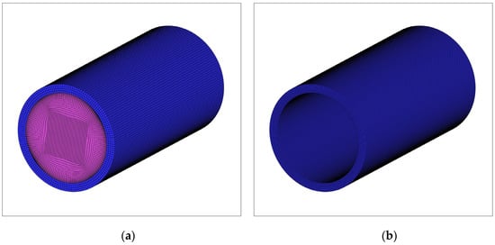
Figure 2.
Computation meshes for the numerical procedure. (a) Meshes for temperature analysis. (b) Meshes for thermal stress analysis.
Based on the deterministic, coupled thermal—structural model of the receiver tube, the model output can be obtained and expressed as:
where y is the maximum temperature or thermal stress inside the tube wall as the deterministic model’s output, and p1, p2, … pk are uncertain input parameters. The maximum temperature inside the tube wall as the model output is a function of seven parameters (k = 7), whereas the maximum thermal stress inside the tube wall as the model output is a function of nine parameters (k = 9). The uncertain input parameters remain unchanged in the deterministic model.
3. Uncertainty Analysis Model
3.1. Characteristics of the Uncertainties
To conduct an uncertain analysis of the temperature and thermal stress for the receiver tube, the first step is to select the uncertainties. For the boundary conditions of the receiver tube, the peak incident heat flux on the tube wall is a typical uncertain parameter, which is influenced by the level of direct normal irradiance. For the heat loss of the receiver tube, the proportion of the reflection heat loss is obviously larger than that of the radiation and convection heat loss. Consequently, the uncertainty of the tube coating absorptivity is taken into account, while the tube coating emissivity, the convective heat transfer coefficient outside the tube wall, and the ambient temperature are given specific values. For the thermophysical properties of the heat transfer fluid and the tube material, the measurement error of the density is smaller than that of other properties. Therefore, the uncertainties of the thermophysical properties of the tube material and the heat transfer fluid are all considered except for their densities. The central values and uncertainty probability distributions of nine uncertain input parameters are given in Table 1.

Table 1.
Central values and uncertainty probability distributions of input uncertainties.
3.2. Uncertainty Propagation
The conceptual representation of the uncertainty propagation is demonstrated in Figure 3. It demonstrates that the dispersions of the model outputs of the maximum temperature and thermal stress inside the receiver tube wall can be attributed to the input uncertainties. Due to high accuracy, the MC simulation method [33] is applied to conduct uncertainty propagation and determine the dispersion of the model output. The calculation steps of the MC simulation method are given below:
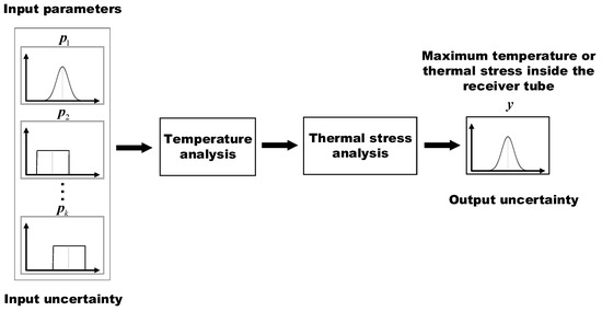
Figure 3.
Conceptual representation of uncertainty propagation.
- The probability distributions of the uncertainties are given;
- The sample size N is specified for the MC simulation;
- An appropriate sampling method is chosen. There are several methods for sampling probability distributions, such as random sampling, Latin Hypercube sampling, and Sobol sampling [34]. Rather than generating random numbers, the Sobol sampling method generates a uniform distribution in probability space. As a result, the Sobol sampling method is more accurate than other sampling methods and, therefore, was selected in this paper. The result of this step is to construct a matrix that contains the sampled values of the uncertain input parameters, which can be expressed as follows:
- Based on the sampled values of the uncertain input parameters, the temperature and thermal stress simulation procedures are repeated N times. The dispersion of the model output can be obtained and expressed as follows:
3.3. Approximation Model
In the process of the uncertainty propagation analysis, a calculation complexity problem exists for the numerical simulation procedure of the temperature and thermal stress analyses. Therefore, the complex temperature and thermal stress models should be surrogated by the approximation model, which develops the relationship between the uncertain input parameters and the response with equations. There are various approximation models, such as the response surface model, the Kriging model, and the neural network model. In this paper, the response surface model [35] was chosen because of its low computational cost and great applicability. Then, the relationship between the uncertain input parameters and the response is fitted with a polynomial equation and expressed as follows:
where is the approximate model output; is the regression coefficient, which can be obtained by the least square method; is the basic function of ; and M is the number of terms of .
To measure the reliability of the approximation function for the receiver tube model under multi-source uncertainties, the coefficient R2 is used to conduct an error analysis and calculated as follows:
where and are, respectively, the actual and approximate model outputs; is the average value of the actual model output; n is the sample size for building the response surface model.
Due to the advantages of high efficiency, the optimal Latin hypercube (OLH) sampling method [36] was adopted to gain the sampling points of the uncertain input parameters for the response surface model construction. In total, 146 sampling points were chosen to construct an approximation model of the receiver tube model under multi-source uncertainties, and 73 sampling points were chosen to perform the error analysis. The error analysis results of the model outputs of the maximum temperature and thermal stress inside the tube wall are, respectively, shown in Figure 4 and Figure 5. The results demonstrated that the approximation values were consistent with the simulation values for model outputs of the maximum temperature and thermal stress inside the tube wall, with R2 values of 1 and 0.9883, respectively.
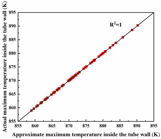
Figure 4.
Error analysis results of the maximum temperature inside the tube wall as the model output.
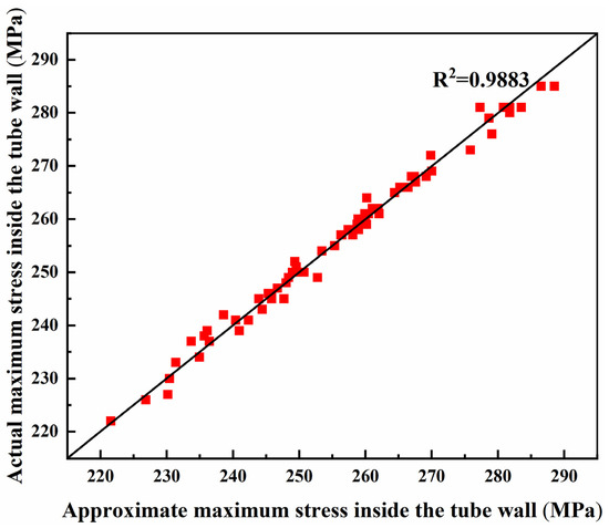
Figure 5.
Error analysis results of the maximum stress inside the tube wall as the model output.
4. Results and Discussion
4.1. Deterministic Model Validation
To validate the accuracy of the deterministic, coupled thermal–structural model, the simulation results of this paper were compared with other findings reported in the literature. For the thermal analysis model validation, the length of the receiver tube was 3 m with an inner/outer radius of 10.5/12.5 mm. The inlet fluid parameters and the heat flux distribution are in accord with that of Du et al. [2]. The temperature analysis results of this paper and those reported by Du et al. [2] are shown in Figure 6. The comparison demonstrates that the simulation results of this paper and those of Du et al. [2] are in good agreement, and the maximum relative error of the temperature in this study was only 1.12%.
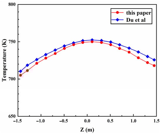
Figure 6.
Temperature analysis results of this paper and those indicated by Du et al. [2].
For the thermal stress analysis, the geometry of the receiver tube was the same as the above. The inner and outer tube wall temperatures were, respectively, 700 K and 750 K, which indicates that only the radial temperature gradient was considered. The simulation results of this paper were compared with the theoretical equation results of Timošenko et al. [12] and are shown in Figure 7. The comparison of the results proves that the thermal stress analysis model also has good reliability.
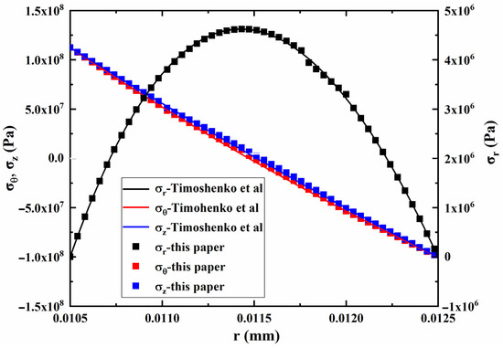
Figure 7.
Thermal stress analysis results of this paper and those of Timošenko et al. [12].
4.2. Simulation Results of the Deterministic Model
Based on the deterministic model, the temperature and thermal stress distributions of the receiver tube wall were obtained and are depicted in Figure 8 and Figure 9, respectively. The results revealed that the temperature distribution of the tube wall was similar to that of the incident solar heat flux distribution, which demonstrated that the incident heat flux distribution had a large influence on the temperature distribution of the tube wall. Consequently, the maximum temperature of the tube wall was 871 K and occurred at the center of the outer sunward tube wall, which was in accord with the peak incident heat flux location.
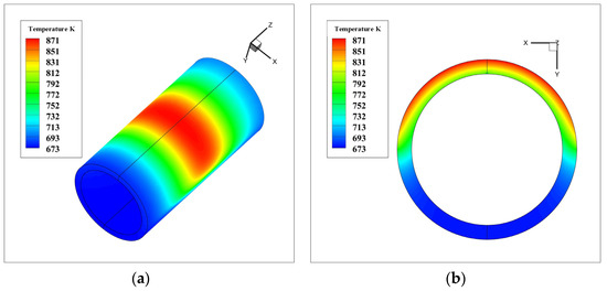
Figure 8.
Temperature distribution of the tube. (a) Whole tube wall (z = 1:60); (b) Cross-wall of the tube (z = 0 m).
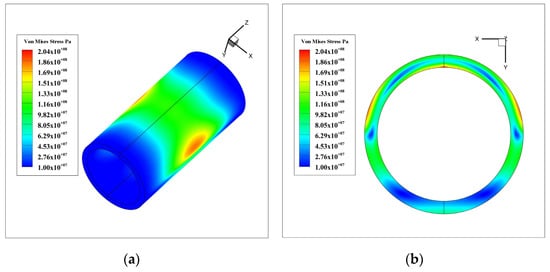
Figure 9.
Thermal stress distribution of the tube. (a) Whole tube wall (z = 1:60); (b) Cross-wall of the tube (z = 0 m).
The thermal stress distribution of the tube wall was different from that of the temperature distribution because the thermal stress is usually decided by the temperature gradient. As a result, the maximum thermal stress of the tube wall was 204 MPa and was located at the center of the inner sunward tube wall.
4.3. Comparison Results of the Uncertainty Analysis and Deterministic Models
To investigate the dispersions of the model outputs of the maximum temperature and thermal stress inside the receiver tube wall under multi-source uncertainties, an uncertainty propagation evaluation was performed through MC simulations using 5000, 10,000, and 15,000 samples. The results showed that there was no appreciable difference in the cumulative frequency of the model output when the sample size exceeded 10,000. Therefore, 10,000 samples were used to conduct the uncertainty propagation analysis.
The frequency and cumulative frequency of the maximum temperature and thermal stress inside the tube wall under uncertainty are, respectively, shown in Figure 10 and Figure 11. Figure 10 demonstrates that the lower and upper bounds of the maximum temperature inside the tube wall under uncertainty were, respectively, 847 K and 895 K, with an expectation of 871 K and a standard deviation of 8 K. The deterministic result of the maximum temperature inside the tube wall (871 K) is also depicted in Figure 10, and the corresponding cumulative frequency was 50%. This demonstrates that there was a 50% probability that the maximum temperature of the tube wall under uncertainty would be more than the deterministic value of 871 K, and the maximum deviation of the uncertainty analysis result from the deterministic value was 24 K, which may cause the overheating of the receiver. As a result, to prevent receiver failure caused by overheating, the dispersion of the maximum temperature inside the tube wall under uncertainty should be considered in the design process of the receiver.
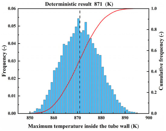
Figure 10.
Probability distribution of the maximum temperature inside the tube wall under uncertainty.
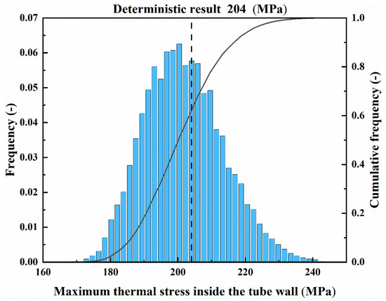
Figure 11.
Probability distribution of the maximum thermal stress inside the tube wall under uncertainty.
Figure 11 illustrates the lower and upper maximum thermal stresses inside the tube wall under uncertainty, which were, respectively, 173 MPa to 245 MPa, with an expectation of 204 MPa and a standard deviation of 12 MPa. The results demonstrated that there was a 50% probability of achieving maximum thermal stress exceeding 200 MPa and a 25% probability of achieving maximum thermal stress exceeding 208 MPa. The deterministic result of the maximum thermal stress inside the tube wall is also plotted in Figure 11, which shows a 40% probability of exceeding the deterministic result of the maximum thermal stress inside the tube wall (204 MPa), and the maximum deviation of uncertainty analysis result from the deterministic value was 41 MPa, which may cause fatigue damage in the receiver. It is worth noting that although the probability distributions of the uncertain input parameters in this paper were all symmetrical, the deterministic result of the maximum thermal stress was not at the cumulative frequency of 50%. This can be attributed to nonlinear models and responses. All in all, considering that the model input parameters generally have uncertainties, the adaptability of the deterministic model has to be questionable. Thus, to prevent fatigue damage in the receiver tube wall caused by the dispersion of the thermal stress inside the tube wall, the thermal stress analysis modeling of the receiver tube wall under multi-source uncertainties is strongly recommended for the receiver design.
4.4. Sensitivity Analysis of Uncertainties
Due to high accuracy, Sobol’s global sensitivity method [37] was used to obtain those input parameters that were most important to the model output. For this technique, the total sensitivity index ST of each input parameter is calculated to denote the effects of an input parameter and all its interactions on the model output. Consequently, the higher the total sensitivity index ST, the more sensitive the input parameter is to the model output.
The sensitivity analysis results of the maximum temperature inside the tube wall are depicted in Figure 12. These results demonstrated that the peak incident solar flux p1 was the most sensitive to the maximum temperature inside the tube wall with a total sensitivity index ST of 0.8081 and a contribution rate of 80.81%. The reason can be attributed to the great impact of the incident solar flux on the temperature distribution of the tube wall, as discussed in Section 4.2. Except for the peak incident solar flux p1, the contribution rate of the thermal conductivity of molten salt p5 was the largest, at 8.55%. This is because the effect of the thermal conductivity of molten salt p5 on the heat transfer process of the receiver tube was large. Figure 12 also shows that the specific heat of tube material p6 almost had no effect on the maximum temperature inside the tube wall with a total sensitivity index ST and contribution rate of nearly 0. This may be attributed to the thin wall thickness of the receiver tube.
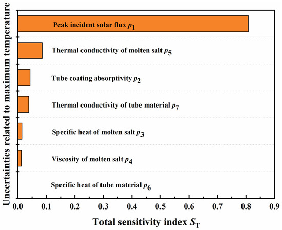
Figure 12.
Sensitivity analysis results of the maximum temperature inside the tube wall.
Figure 13 shows the sensitivity analysis results of the maximum thermal stress inside the tube wall. It is observed that the impact of the peak incident solar flux p1 on the maximum thermal stress inside the tube wall was also the largest, followed by the elastic modulus of the tube material p9, the thermal expansion coefficient of the tube material p8, and thermal conductivity of the tube material p7, with total sensitivity indexes ST of 0.5609, 0.1629, 0.1412, 0.1015 and contribution rates of 55.53%, 16.13%, 13.98%, 10.05%, respectively. Consequently, the above four input parameters accounted for 95.69% of the total contributions. In addition, the results showed that the specific heat of the tube material p6 was the least sensitive to the maximum thermal stress of the tube wall, with a total sensitivity index ST and contribution rate of nearly 0.
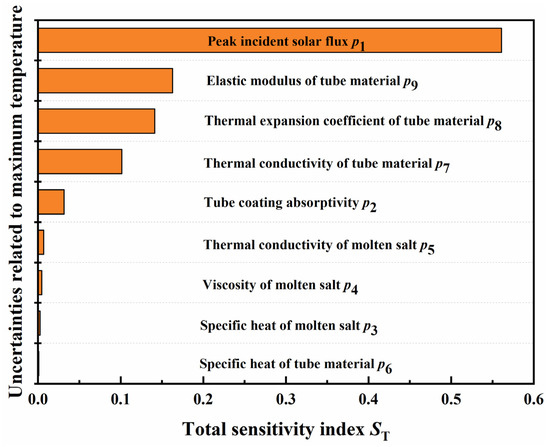
Figure 13.
Sensitivity analysis results of the maximum stress inside the tube wall.
5. Conclusions
Based on a coupled thermal–structural model and the uncertainty propagation analysis method, the dispersions of the maximum temperature and thermal stress inside a receiver tube wall under multi-source uncertainties were presented, allowing us to provide additional reliability in the process of the SPT molten salt receiver design. The results revealed the following findings:
- (1)
- The maximum temperature inside the tube wall under multi-source uncertainties ranged from 847 K to 895 K with an expectation of 871 K and a standard deviation of 8 K. The results demonstrated that there was a 50% probability that the maximum temperature of the tube wall under uncertainty would be more than the deterministic value of 871 K, and the maximum deviation of the uncertainty analysis result from the deterministic value was 24 K, which may cause the overheating of the receiver.
- (2)
- The maximum thermal stress inside the tube wall under multi-source uncertainties ranged from 173 MPa to 245 MPa, with an expectation of 204 MPa and a standard deviation of 12 MPa. The results demonstrated that there was a 40% probability of exceeding the deterministic result of the maximum thermal stress inside the tube wall (204 MPa), and the maximum deviation of uncertainty analysis result from the deterministic value was 41 MPa, which may cause fatigue failure in the receiver.
- (3)
- The global sensitivity results indicated that the peak incident solar flux was the most sensitive to the maximum temperature and thermal stress inside the tube wall with contribution rates of 80.81% and 55.53%, respectively. Furthermore, the elastic modulus, the thermal expansion coefficient, and the thermal conductivity of the tube material also had great effects on the maximum thermal stress inside the tube wall, with contribution rates of 16.13%, 13.98%, and 10.05%, respectively.
Author Contributions
Methodology, Y.L.; software, G.L.; validation, Z.W.; investigation, Z.W.; data curation, G.L.; writing—original draft preparation, Y.L.; writing—review and editing, T.L.; funding acquisition, Y.L. All authors have read and agreed to the published version of the manuscript.
Funding
This research was funded by the National Natural Science Foundation of China (No. 51806009) and the State Key Laboratory of Clean Energy Utilization (No. ZJU-CEU2020019).
Conflicts of Interest
The authors declare no conflict of interest.
References
- Yu, Q.; Fu, P.; Yang, Y.; Qiao, J.; Wang, Z.; Zhang, Q. Modeling and parametric study of molten salt receiver of concentrating solar power tower plant. Energy 2020, 200, 117505. [Google Scholar] [CrossRef]
- Du, B.C.; He, Y.L.; Zheng, Z.J.; Cheng, Z.D. Analysis of thermal stress and fatigue fracture for the solar tower molten salt receiver. Appl. Therm. Eng. 2016, 99, 741–750. [Google Scholar] [CrossRef]
- Conroy, T.; Collins, M.N.; Grimes, R. A review of steady-state thermal and mechanical modelling on tubular solar receivers. Renew. Sustain. Energy Rev. 2020, 119, 109591. [Google Scholar] [CrossRef]
- Ortega, J.; Khivsara, S.; Christian, J.; Ho, C.; Yellowhair, J.; Dutta, P. Coupled modeling of a directly heated tubular solar receiver for supercritical carbon dioxide Brayton cycle: Optical and thermal-fluid evaluation. Appl. Therm. Eng. 2016, 109, 970–978. [Google Scholar] [CrossRef]
- Yang, X.; Yang, X.; Ding, J.; Shao, Y.; Fan, H. Numerical simulation study on the heat transfer characteristics of the tube receiver of the solar thermal power tower. Appl. Energy 2012, 90, 142–147. [Google Scholar] [CrossRef]
- Liu, Y.; Ye, W.J.; Li, Y.H.; Li, J.F. Numerical analysis of inserts configurations in a cavity receiver tube of a solar power tower plant with non-uniform heat flux. Appl. Therm. Eng. 2018, 140, 1–12. [Google Scholar] [CrossRef]
- Wang, K.; Jia, P.S.; Zhang, Y.; Zhang, Z.D.; Wang, T.; Min, C.H. Thermal-fluid-mechanical analysis of tubular solar receiver panels using supercritical CO2 as heat transfer fluid under non-uniform solar flux distribution. Sol. Energy 2021, 223, 72–86. [Google Scholar] [CrossRef]
- Sánchez-González, A.; Rodríguez-Sánchez, M.R.; Santana, D. Aiming strategy model based on allowable flux densities for molten salt central receivers. Sol. Energy 2017, 157, 1130–1144. [Google Scholar] [CrossRef]
- Sánchez-González, A.; Rodríguez-Sánchez, M.R.; Santana, D. Allowable solar flux densities for molten-salt receivers: Input to the aiming strategy. Results Eng. 2020, 5, 100074. [Google Scholar] [CrossRef]
- Nithyanandam, K.; Pitchumani, R. Thermal and structural investigation of tubular supercritical carbon dioxide power tower receivers. Sol. Energy 2016, 135, 374–385. [Google Scholar] [CrossRef]
- Young, W.C.; Budynas, R.G.; Sadegh, A.M. Roark’s Formulas for Stress and Strain; McGraw-Hill: New York, NY, USA, 2012. [Google Scholar]
- Timošenko, S.P. Theory of Elasticity; McGraw-Hill: New York, NY, USA, 1951. [Google Scholar]
- Kim, J.S.; Potter, D.; Gardner, W.; Too, Y.C.S.; Padilla, R.V. Ideal heat transfer conditions for tubular solar receivers with different design constraints. In Proceedings of the AIP Conference Proceedings, Bikaner, India, 24–25 November 2017. [Google Scholar]
- Conroy, T.; Collins, M.N.; Fisher, J.; Grimes, R. Levelized cost of electricity evaluation of liquid sodium receiver designs through a thermal performance, mechanical reliability, and pressure drop analysis. Sol. Energy 2018, 166, 472–485. [Google Scholar] [CrossRef]
- Peng, K.; Qin, F.G.; Jiang, R.; Kang, S. Effect of tube size on the thermal stress in concentrating solar receiver tubes. J. Sol. Energy Eng. 2020, 142, 51008. [Google Scholar] [CrossRef]
- Ortega, J.; Khivsara, S.; Christian, J.; Ho, C.; Dutta, P. Coupled modeling of a directly heated tubular solar receiver for supercritical carbon dioxide Brayton cycle: Structural and creep-fatigue evaluation. Appl. Therm. Eng. 2016, 109, 979–987. [Google Scholar] [CrossRef]
- Wan, Z.; Fang, J.; Tu, N.; Wei, J.; Qaisrani, M.A. Numerical study on thermal stress and cold startup induced thermal fatigue of a water/steam cavity receiver in concentrated solar power (CSP) plants. Sol. Energy 2018, 170, 430–441. [Google Scholar] [CrossRef]
- Montoya, A.; Rodríguez-Sánchez, M.R.; López-Puente, J.; Santana, D. Numerical model of solar external receiver tubes: Influence of mechanical boundary conditions and temperature variation in thermoelastic stresses. Sol. Energy 2018, 174, 912–922. [Google Scholar] [CrossRef]
- Wang, W.Q.; Li, M.J.; Cheng, Z.D.; Li, D.; Liu, Z.B. Coupled optical-thermal-stress characteristics of a multi-tube external molten salt receiver for the next generation concentrating solar power. Energy 2021, 233, 121110. [Google Scholar] [CrossRef]
- Silva, R.; Pérez, M.; Berenguel, M.; Valenzuela, L.; Zarza, E. Uncertainty and global sensitivity analysis in the design of parabolic-trough direct steam generation plants for process heat applications. Appl. Energy 2014, 121, 233–244. [Google Scholar] [CrossRef]
- Muller, S.C.; Remund, J. Solar Radiation and Uncertainty Information of Meteonorm 7. In Proceedings of the 26th European Photovoltaic Solar Energy Conference and Exhibition, Hamburg, Germany, 5–9 September 2011; pp. 4388–4390. [Google Scholar]
- Ho, C.K.; Kolb, G.J. Incorporating Uncertainty into Probabilistic Performance Models of Concentrating Solar Power Plants. J. Sol. Energy Eng. 2010, 132, 533–542. [Google Scholar] [CrossRef]
- Ho, C.K.; Khalsa, S.S.; Kolb, G.J. Methods for probabilistic modeling of concentrating solar power plants. Sol. Energy 2011, 85, 669–675. [Google Scholar] [CrossRef][Green Version]
- Janz, G.J.; Tomkins, R.P.T. Molten Salts Data on Additional Single and Multi-component Salt Systems. In Number IV in Physical Properties Data Compilations Relevant to Energy Storage; U.S. Government Printing Office: Washington, DC, USA, 1981. [Google Scholar]
- Jiang, L.; Ye, J. Quantifying the effects of various uncertainties on seismic risk assessment of CFS structures. Bull. Earthq. Eng. 2020, 18, 241–272. [Google Scholar] [CrossRef]
- Luo, Z.X.; Shi, Q.H.; Wang, L. Size-Dependent Mechanical Behaviors of Defective FGM Nanobeam Subjected to Random Loading. Appl. Sci. 2022, 12, 9896. [Google Scholar] [CrossRef]
- Zhou, X.Y.; Wang, N.W.; Xiong, W.; Wu, W.Q.; Cai, C.S. Multi-scale reliability analysis of FRP truss bridges with hybrid random and interval uncertainties. Compos. Struct. 2022, 297, 115928. [Google Scholar] [CrossRef]
- Wang, J.N.; Li, X.; Chang, C. Analysis of the influence factors on the overheat of molten salt receiver in solar tower power plants. Proc. CSEE 2010, 30, 107–114. [Google Scholar]
- Luo, Y.; Du, X.; Wen, D. Novel design of central dual-receiver for solar power tower. Appl. Therm. Eng. 2015, 91, 1071–1081. [Google Scholar] [CrossRef]
- Cheng, Z.D.; He, Y.L.; Cui, F.Q.; Xu, R.J.; Tao, Y.B. Numerical simulation of a parabolic trough solar collector with nonuniform solar flux conditions by coupling FVM and MCRT method. Sol. Energy 2012, 86, 1770–1784. [Google Scholar] [CrossRef]
- Fauple, J.H.; Fisher, F.E. Engineering Design—A Synthesis of Stress Analysis and Material Engineering; Wiley: New York, NY, USA, 1981. [Google Scholar]
- Zavoico, A.B. Solar Power Tower Design Basis Document; Sandia National Laboratories: Albuquerque, NM, USA, 2001. [Google Scholar]
- Robert, C.; Casella, G. Monte Carlo Statistical Methods; Springer: Cham, Switzerland, 2013. [Google Scholar]
- Saltelli, A.; Ratto, M.; Andres, T.; Campolongo, F.; Cariboni, J.; Gatelli, D.; Saisana, M.; Tarantola, S. Global Sensitivity Analysis: The Primer; John Wiley & Sons: Chichester, UK, 2008. [Google Scholar]
- Mäkelä, M. Experimental design and response surface methodology in energy applications: A tutorial review. Energy Convers. Manag. 2017, 151, 630–640. [Google Scholar] [CrossRef]
- Devanathan, S.; Koch, P.N. Comparison of meta-modeling approaches for optimization. In Proceedings of the ASME International Mechanical Engineering Congress and Exposition, Denver, CO, USA, 11–17 November 2011; Volume 54891, pp. 827–835. [Google Scholar]
- Sobo, I.M. Sensitivity estimates for nonlinear mathematical models. Math. Model. Comput. Exp. 1993, 1, 407–414. [Google Scholar]


Publisher’s Note: MDPI stays neutral with regard to jurisdictional claims in published maps and institutional affiliations. |
© 2022 by the authors. Licensee MDPI, Basel, Switzerland. This article is an open access article distributed under the terms and conditions of the Creative Commons Attribution (CC BY) license (https://creativecommons.org/licenses/by/4.0/).