Abstract
In scientific journals, it is increasingly common to find articles presenting methods for solving problems not based on idealistic mathematical models containing perfectly accurate coefficient values that cannot be obtained in practice, but on models in which coefficient values are affected by uncertainty and are expressed in the form of intervals, fuzzy numbers, etc. However, solving tasks with interval coefficients is not fully mastered, and a number of such problems cannot be solved by currently known methods. There is undeniably a research gap here. The article presents a method for solving problems governed by the quadratic interval equation and shows how to find the tolerant optimal control value of such a system. This makes it possible to solve problems that could not be solved before. The paper introduces a new concept of the degree of robustness of the control to the set of all possible multidimensional states of the system resulting from its uncertainties. The method presented in the article was applied to an example of determining the optimal value of nitrogen fertilization of a sugar beet plantation, the vegetation of which is under uncertainty. It would be unrealistic to assume precise knowledge of crop characteristics here. The proposed method allows to determine the value of fertilization, which gives a chance to obtain the desired yield for the maximum number of field conditions that can occur during the growing season.
1. Introduction
Scientists, engineers, and practitioners have been trying to apply classical mathematics to solving real problems for centuries. However, this mathematics requires precise knowledge of both the formulas describing the dependencies existing in the system and the exact values of the coefficients occurring in them. Unfortunately, in real systems, we often do not fully know either one or the other. For this reason, classical mathematics is sometimes not suitable for solving real problems, which makes scientists try to develop new mathematical methods capable of analyzing and processing uncertain, approximate data, e.g., interval, fuzzy data, etc.
An example of the problem with uncertainty is presented in [1]. It concerns vendor selection and supply chain management. The problem describes a complex delivery system whose future behavior cannot be accurately predicted. Taking into account the uncertainty of this system, it is true that only uncertain results can be obtained. But the results are realistic and do not introduce the illusion of accuracy, which in this case is unattainable. The second example of an uncertain problem is the task of making optimal decisions presented in [2]. Decision optimization in the conditions of having uncertain data (here fuzzy) requires the use of more sophisticated mathematical methods than in the case of precise data.
Various mathematical forms of defining uncertain data are used in science. However, the most commonly used form is the interval. Confirmation of this truth is provided by articles such as [3,4] recently published in Applied Sciences. In [3] the authors apply interval analysis to the complicated problem of heat and mass transfer. It is a problem where it is difficult to find exact data values. Another very practical example of using intervals is the behavior analysis of a two-pole generator rotor systems [4].
The authors of this article have been dealing with solving uncertainty problems with particular emphasis on equations for many years. Solving uncertain equations is a much more difficult task than calculating the values of uncertain functions. In an article [5] published in 2022 in Applied Sciences, the authors presented a way to realistically solve the basic interval equation based on the newly introduced concept of control value robustness to a set of possible, uncertain system states.
The task of solving interval and fuzzy quadratic equations is very complicated and has been dealt with by many scientists. It should be remembered here that an interval is a special case of a fuzzy set whose membership function is rectangular. Hence, the methods of solving fuzzy equations can be used to solve interval equations. Further on, the solution of the quadratic interval equation (QIE) in the form (1) will be discussed.
Equation of type (1) will be applied further in solving the problem of fertilizing plants. Solving interval equations (IE) and fuzzy equations (FE) is a very difficult task, as the history of their research has shown. Already W. Oetli wrote about it in 1964 and 1965 [6,7] and D. Gay in 1982 [8]. They emphasized that one of the reasons may be the multidimensional nature of the solution ( space) and the complicated and non-convex shape of the set of possible solutions. In recent years it was also pointed out by Lodwick and Dubois in [9] and Dymova and Sevastyanov in [10,11], who state that in the case of nonlinear, quadratic interval equations “to date there are no universal methods for solving such equations and that the problem is open”. The difficulties with solving linear and nonlinear IEs and FEs are also well presented in the articles of Buckley [12,13,14,15]. He notes the difference in arithmetic operations performed by classical and fuzzy arithmetic: “a major problem in solving FEs: some basic operations we use to solve crisp equations do not hold for FEs. Actually, this comes as no great surprise because this also happens in probability theory”.
Analyzing the history of research on IEs, it can be stated that the authors of subsequent articles always analyzed the methods of their predecessors, detected their weaknesses and tried to improve them in their methods. In this way, they realized scientific progress. They also introduced new definitions and concepts regarding IEs. For example, Barth and Nuding in [16] introduced the concept of ‘set of solutions’ and the optimal interval enclosure of the IEs system . An important item in the solving interval equations is the article [9] by Lodwick and Dubois. They draw attention to the fact that “almost from the start of fuzzy linear system research, various anomalies arose, which in our opinion, are from an incomplete or lack of understanding of interval linear equations”. They add that the resultant intervals are sometimes improper, and therefore unrealizable, and in the case of fuzzy equations, the solutions provided include at some -levels intervals, which are not nested. Lodwick and Dubois have proposed their own method for solving linear IEs that returns either an empty interval or a proper interval, and never an improper one. In [10] Dymova at al. emphasize the need to find algebraic (equality type) solutions of IEs: “Usually interval type computation packages deliver united, tolerance and control solutions of interval equations. But the practical need exists for algebraic solutions (both sides of equations are equal)”. Sometimes the interval system does not have an algebraic (equality type) solution. What is then to do? The authors of the article provide specific advice.
In [17], Dymova and Sevastyanov draw attention to anomalies arising when solving quadratic interval equations (QIE) and quadratic fuzzy equations (QFE) with known methods, e.g., excess width effect or too wide intervals or fuzzy values representing final solutions and achieving inverted (improper) intervals as solutions. They propose an approach of ‘interval extended zero’ for alleviating observed problems. In [17] this method was used to solve the QIE (2) where means an ‘extended zero’ introduced instead of crisp 0.
They also show an example of solving the equation which, according to authors of the article [12], did not have a negative root. The method of ‘interval extended zero’ showed the existence of such a root. It should be noted here that the authors of [17] assume in advance that the solution of a QIE is a 1-dimensional interval .
In [18] Allahviranloo and Moazam provide the solution method of the full fuzzy quadratic equation , based on the optimization theory. The method finds roots of equations. Its advantage is that the complexity level of the solution does not depend on whether the coefficients A, B are positive or negative. Allahviranloo and Ghanbari in [19] propose an analytical method of obtaining algebraic solutions of fuzzy linear systems based on the concept of ‘interval inclusion linear system’. They show examples of solving of FE with 3 variables. The solutions are 2D fuzzy numbers (FN).
In [20] Allahviranloo et al. show with a counterexample that the weak solution of a fuzzy linear system defined by Friedmann et al. in the paper [21] is not always a fuzzy number vector because one of its components can be a non-realizable fuzzy number. This article is one of the many pieces of evidence of difficulties in solving systems of FEs found in the scientific literature. In an interesting article [22], V. Kreinovich draws attention to the basic, but rarely analyzed in literature, problem of the dependence of the obtained solutions of uncertain equations on the practical requirements for the solution. The article states “we need to use different techniques depending on the original practical problem”. His observations indicate difficulties in developing one universal method of solving IEs systems.
In [23] M. Landowski shows how to find the roots of QIE using the multidimensional interval arithmetic (MIA). These roots are algebraic solutions, i.e., after inserting them into the equation to be solved, we obtain the equality of the left and right sides of the equation. The article explains the difference between the multidimensional concept of a root and its span. Typically, this span is misinterpreted in articles as algebraic root. The author of the article shows that, contrary to some opinions, it is possible to define algebraic roots of uncertain quadratic equations.
Apart from analytical methods of solving uncertain linear and nonlinear equations [9,10,11,12,13,14,15,16,17,18,19,23,24,25,26,27] numerical methods have also been developed (e.g., [28,29,30,31,32,33,34,35,36]). Numerical methods began to be developed after the shortcomings of early analytical methods, such as those presented by Buckley, were discovered [12,13,15]. Numerical methods have also been developed in the last (2016–2021) years [28,29,30,31,37]. These methods try to find the roots of equations approximately. This can be done, for example, by the search method. It turns out, however, that these methods are not perfect, and scientists are constantly working on new methods. In [24] Hasan et al. propose an analytical method of solving QFEs without the use of -cuts. Instead, they use the distribution function and the complementary distribution function. This article shows the possibility of using various alternative methods for solving uncertain nonlinear equations.
The problem of solving nonlinear interval and fuzzy equations should not be considered as fully solved and the existing methods as ideal. Scientists are not satisfied with them and are constantly looking for new and better methods. The recent publications [38,39,40] are the proof of this state. They are testimony to the difficulty of matter. Uncertainties in problems greatly increase the scale of theoretical and computational difficulties that need to be overcome in order to solve the problem. This sometimes leads to controversial results, such as those presented in [38], where some of the resulting ‘fuzzy numbers’ do not meet the requirements of the fuzzy number definition, e.g., the requirement to meet the inclusion principle of fuzzy arithmetic results [41].
Summarizing the conducted analysis of publications in the field of QIEs and the search for their tolerance solutions, it can be stated that there is still a research gap. This gap in the field of tolerance control of static systems defined by the quadratic Equation (1) (as well as lower- and higher-order equations) is that for many cases of systems (this depends on numerical values of intervals on the left side of the equation and the tolerance interval on the right), existing methods cannot find any solution at all. Thus, there is a need to develop such a method for determining the value of realistic tolerance control, which will find the best value of control x for any systems, regardless of the numerical interval values.
The scientific contributions (novelty) that characterize the method described in our article are listed below.
- Dropping the idealistic requirement that every possible value of control x of a system governed by an interval quadratic relation, always, at every possible state of the system , satisfies the condition .This is because absolute satisfaction of this condition is usually impossible due to the presence of as many as three uncertainty generators , , on the left side of the equation. Hence, usually the uncertainty of the entire left side of the equation is, regardless of the chosen numerical control value x, much larger than the tolerance of on the right side of the equation.
- Introducing for the first time concepts of: robust tolerant solution and robustness of the chosen control value x for static interval control systems.The robustness informs at how large part of all possible states of the system, the considered numerical value of control x will fulfill the task of tolerant control. In practical tasks, it is rarely possible to find a control x that meets the requirement of tolerant control under all possible states of an uncertain system. In our article, we showed how to apply this new concept of robustness to an interval quadratic system.
The main difference between existing methods of solving tolerance control tasks and our method is that existing methods of solving tasks always try to find ideal tolerance control, which rarely exists in practice. If they do not find such a solution, they simply report that it does not exist. On the other hand, our method makes it possible to find both an ideal tolerant solution and a robust control with the highest value of robustness . Thus, it makes it possible to find a solution even in problems where previous methods have failed.
In the case of the problem of optimal fertilization of plants, the article shows how to determine the value of optimal fertilization using the robustness method. The method can be applied also in mechanical, electrical, biological, medical and other systems. All these systems use mathematical modeling of the dependencies occurring in them with the use of polynomials of various degrees, including square ones. The advantage of polynomials is that the coefficients appearing in them are easy to identify on the basis of measurement data. Uncertain polynomial relationships, including quadratic ones, describe, for example, the paths of missiles fired from guns, the range of these missiles, the paths of rockets, airplanes, ships, water objects, etc.
One of the greatest limitations in applying the method is probably the difficulty of understanding it, resulting from its multidimensional nature. There are 5 uncertain variables () in the interval uncertain quadratic system described by the Equation (1). This makes it impossible to visualize the problem, easily explain how to solve it, and makes it difficult to understand. Therefore, in our article (in Section 3), we presented a visualization and a way to solve a simplified version of the equation that can be represented and explained in 2D space. Based on the visualization of the problem with 3 uncertain variables (), it can be easier to solve a 5-dimensional problem.
The motivation behind this article was to show that it is possible to solve such QIEs, which so far could not be solved, and the way to this goal is the concept of robustness of the control (decision) x to the set of possible states of an uncertain system and the use of MIA.
Further on in the article, a brief introduction to MIA will be presented first in Section 2. In Section 3, the important concept of control robustness with respect to the set of possible, uncertain system states will be explained and in Section 3.1, the algorithm for determining the tolerant control [42,43,44] of the QIE will be briefly presented. Section 4 describes its application to fertilizing the sugar beet cultivation and the Section 4.1 presents a comparison of numerical and geometric methods of solving QIEs and a discussion on the optimal dose of fertilization. Section 5 will be devoted to finding the traditionally understood QIE solution in the form of roots of the equation.
2. Introduction to Multidimensional Interval Arithmetic
Currently, there are many types of interval arithmetic (IA), for an overview see [45]. Examples are: standard interval arithmetic (SIA) of Warmus-Sunaga-Moor, extended IA of Kautcher, non-standard IA of Markov, generalized Hukuhara IA of Stefanini, optimistic IA of Boukezoula and Galichet, instantiated IA of Dubois, constrained IA of Lodwick, single-level constrained IA of Chalco-Cano, requisite constrained IA of Klirr, affine IA of Comba and Stolfi. The common feature of these IAs is the type of the result: it is always the interval – a 1D-mathematical object. Hence, above types of IA can be called 1-dimensional. Meanwhile, as it will be shown in Example 1, IA requires a multidimensional approach.
Example 1.
In the slightly deformed cylindrical tank A there is a certain amount a of water which can not be accurately measured. It can only be roughly estimated from the tank dimensions and the water height as [m]. Water from tank A was poured into tank B (also deformed) and then tap water was added to B in an unknown amount x [m]. Basing on measurements of tank B (inner diameter, height) it was estimated that there is now the amount of water [m] in it. Question: what amount of water x was added to the tank B from the tap? The problem of tanks can be presented in the form of Equation (3).
The next question: how many unknowns does this equation contain? At first glance, there seems to be only 1 unknown x. However, it is not. It contains 3 unknowns: a, x, b. The real value of and of is not known and can be any value in the given intervals. So we are dealing with the problem described by one equation containing as many as 3 unknowns. Is it possible to solve one equation with 3 unknowns? It seems not! And yet! It is possible when we revise a notion of the solution and assume that the solution of a problem is any knowledge about the problem unknowns that we are interested in and that we can determine (calculate, infer). In the tanks’ problem the 3-dimensional solution is the set of triples each of which represents one of possible states of the tank system:
Examples of possible system states are: . The set is called the set of possible states of the tank system. The set is the set of possible values of the result variable x. To solve the problem of tanks, we need to develop mathematical models of the real values of the variables a, b and then calculate x. We know the real, exact amount of water in the tank A: [m] = . This knowledge corresponds to the model (5):
where stands for RDM variable (Relative Distance Measure). Similarly, the model of the real value of the variable b, about which we only know that , can be represented in the form (6).
Given the mathematical models of the real values of variables a and b, it is possible to determine the model of the real value of the variable x representing the knowledge of the true value of added water from the tap:
In Formula (7) it is easy to see that the variable x is not 1-dimensional but that it is a function existing in 3D space. The set of possible states of the tank system is given by Equation (8).
Using all possible values of RDM variables , we can generate all possible triples , i.e., all possible states of the tank system. We can also define various simplified information about this set, such as the span of the set of possible values of the variable x, the distribution of cardinality measure , the center of gravity [46,47,48,49].
Performing arithmetic operations with MIA is quite simple. If we have the interval knowledge of the true values of 2 variables a and b, then the arithmetic operation is performed on mathematical models of these values shown in (9) to calculate the result variable value x (10).
After performing the operation (10) we get 3D result set :
In this set, X means the set of possible values of variable . Span of X can be calculated with (12).
The method of calculating the distribution of cardinality measure and of the center of gravity is given in [46,48,50] and will be shown in further examples. MIA and MFA based on it have 7 following important mathematical properties:
- commutativity law for addition and multiplication,
- associativity law for addition and multiplication,
- existence of neutral elements for addition and multiplication,
- existence of inverse elements for addition and multiplication,
- restoration law for addition and multiplication,
- providing algebraic solutions for interval and fuzzy equations,
- independence of the results from the mathematical form of the problem description.
3. Concept of the Robustness of the Control Value to an Uncertain Disturbance
First, the concept of the control robustness will be explained with a simple real-life example. Let us assume that we have bought an apartment and we want to insure it against certain possible risks. The set of considered risks is as follows: —flooding with water, —apartment fire, —apartment theft. We do not know the probability of individual threats occurring in the new block of flats where we have bought the apartment. We only know that such threats are possible. We can insure an apartment for only one selected risk, for 2 selected risks, or for all 3 risks. Which decision will be the most robust against possible threats? Obviously, the decision to have 2-risk insurance is more robust than 1-risk insurance. Covering 3 risks is a more robust decision for a set of possible risks than covering 2 risks or 1 risk.
As we will see, in complex systems there will be multi-dimensional disturbance states defined by a triple , which are independent from us. It will be necessary to determine such a control value x (making a decision about the control value x) that will ensure the achievement of the control goal with as many system disturbance states as possible. If the number of all possible states of a discrete system is n, and the number of states at which a given control x ensures satisfying the control requirements is m, the robustness of the control value x to the system uncertainty is . The robustness can also be called the degree of adjustment of the x-control value to uncertain states of the system. In the following, the concept of robustness will be used in determining the optimal control x in the problem of plant fertilization, which is described by the full quadratic equation . However, the sense of robustness will be explained here only for the simplified version (13) and (14) of the full quadratic equation.
The simplified version (13) enables the visualization of the problem in 2D space , while the full version of the QIE exists in 4D space.
Step 1. We transfer the conventional form of Equation (14) into the MIA form containing the variables RDM and and solve the equation for x.
Note that the values of the roots and are not independent. They are conjugated by the RDM variables ,. One pair corresponds to one pair of roots.
Step 2. Determine the spans and of both roots (16). Figure 1 shows the relationship between the roots’ intervals and and values of the disturbance a.
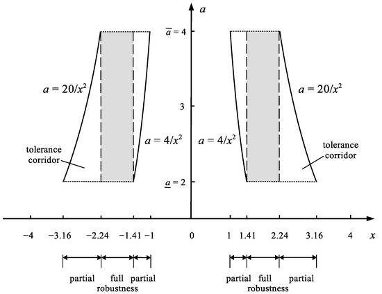
Figure 1.
Illustration of the relationship between the possible values of the roots , and possible values of the uncertain variable a in equation .
Figure 1 shows on the left that the range is the range of solutions x where each value of x gives the value of that hits the tolerance corridor regardless of the true value of the uncertain coefficient a. The condition of the tolerant control , is then fulfilled. Similar is the range of solutions on the right side of Figure 1. Therefore, these ranges are the full robustness ranges (or full fit ranges) of the controls x to uncertainty of the coefficient a. For these ranges the degree of robustness is 1. For the range the values x no longer guarantee the full robustness of the controls x to the uncertainty of the coefficient a. Here only the partial robustness is possible. For the robustness . It is similar for smaller values . Partial (fractional) robustness means that the hit of the value into the tolerance corridor TC = will occur only when the true value of the coefficient a will be included in a part of the range of this coefficient, e.g., for the value of will hit TC = only when . The robustness of the control x informs us about how large fraction of the range makes it possible to hit TC = for the considered value of x. The value of robustness for individual ranges of possible control values x is determined by Formula (17).
Figure 2 shows the distribution of the robustness for individual possible control ranges.
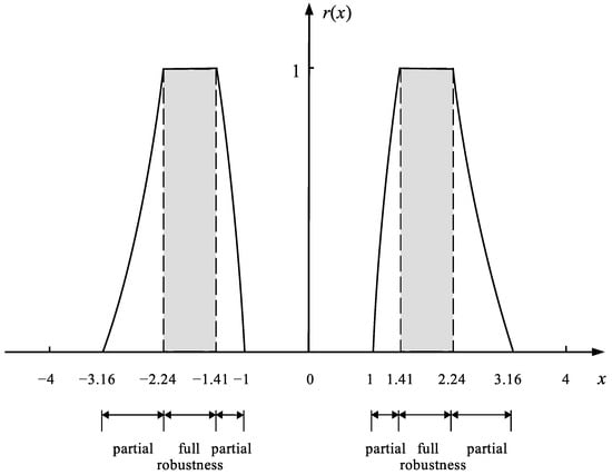
Figure 2.
The distribution of the robustness for possible control values x of the system , where is the tolerance corridor of the control.
As Figure 2 shows, in the case of uncertain system it is possible to find such control values x that give full robustness to the uncertainty of the coefficient . However, Let us now consider another example of a system with smaller TC given by Equation (18).
Solving the problem (18) with the same method, the relationship between the roots and and the uncertain coefficient a is obtained, as shown in Figure 3.
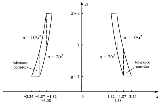
Figure 3.
Illustration of the relationship between the possible roots and and the values of the uncertain coefficient a in the system control task .
As Figure 3 shows, there is no such value of the control x (neither negative nor positive) that would give the full robustness for each possible value of , i.e., a full adjustment of the control x to all possible values of a. Please compare Figure 1 and Figure 3. Individual values of x give only the partial robustness expressed by Formula (19).
The distribution of the robustness for possible negative and positive values of the controls x is shown in Figure 4.
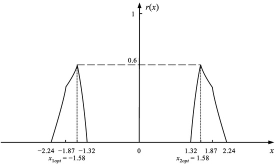
Figure 4.
The distribution of the robustness of possible values of the tolerant control x in the system . Only partially robust control is possible.
As shown in Figure 4, in the system it is not possible to obtain the control x providing the full robustness to the uncertainty of the coefficient . However, there are 2 optimal values and which give the maximum robustness to the uncertainty of a. More precisely, this means that if the true value of the coefficient a of the real system will lie in the range , then the value of will hit the tolerance corridor . If not, it will not hit. The values of and are therefore robust at the degree 0.6 to the whole uncertainty range of a, see Figure 3. Tolerant control can therefore be implemented in this case, although there is no absolute certainty to realize it. Such a situation exists in many real systems. Therefore, it is fully realistic and the control in conditions of incomplete robustness to uncertainty can be called realistic control. The reason for the frequent failure to obtain an ideal tolerant control is the large number of uncertain parameters present in the systems, often a large range of their uncertainty, and high accuracy requirements for the output value y (small range of permissible error). In the system the tolerance range is much larger than in the system .
Both considered systems are a simplified version of the system . In the full version of the quadratic equation, there are not one, but three uncertainty generators: , , . The greater the number of these generators, the smaller the chance of implementing the ideal tolerance control ensuring the certainty of hitting the tolerance corridor . Next, the tolerance control algorithm of the system described by the full quadratic equation will be presented.
3.1. Algorithm for Determining the Tolerant Control of the System
There is given a static system with an input x and an output y realizing the crisp relationship (20).
The knowledge about coefficients of the system is uncertain:
The purpose of the search is to determine one control value x or a set of those values that will allow to obtain the output value y included in the tolerance corridor (22).
The real values of coefficients , , that will appear in a real system are independent from us: they depend on various external factors. They may be called system uncertainty generators (UGs). The intervals , , are epistemic, i.e., only one value is true. Whereas the tolerance corridor is usually defined by the system user depending on his requirements, e.g., technological ones. The task is to determine such a control value (or a set of these values) that will allow to obtain the maximum control robustness for the uncertainty of the coefficients , , . Following steps should be realized to solve the problem.
- Step 1. Transferring the problem to the RDM variables space.
- Step 2. Checking whether the tolerance corridor has been realistically chosen. If it is impossible to obtain results contained in the chosen tolerance corridor, then it should be corrected.
- Step 3. Determining the span of the search range of the control (decision) variable.
- Step 4. Discretization of the span of variable x.
- Step 5. Determining the distribution of the robustness for possible values of control variable x and determining its optimal value with the highest robustness.
4. Determining the Tolerant Solution of the Quadratic Interval Equation on the Example of Fertilizing Sugar Beet Cultivation
Sugar beetroot is an important crop throughout growing regions of many countries. The root of the beet has a sugar content of approximately 17%. In Poland the profit from sugar beetroot cultivation starts at yield [q/ha]. Profitable sugar beet production depends on adequate soil fertility. Using appropriate agrotechnical means some growers receive yield even [q/ha]. Nitrogen (N) is the most yield influencing nutrient and is critical to obtain maximum sugar beet yield and quality. The most common response curve for nitrogen fertilization is shown in Figure 5.
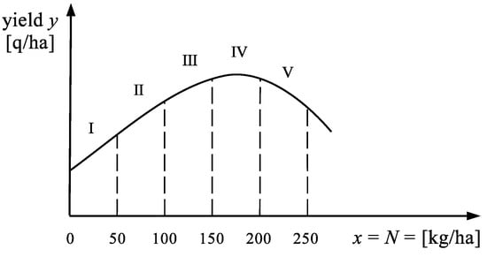
Figure 5.
The typical response curve for nitrogen fertilization x.
Note that the field characteristic in Figure 5 is only an exemplary one. Each field has more or less different characteristics. In addition, the characteristics of one and the same field changes each year depending on the weather situation, insolation, rainfall, average temperatures in the area of cultivation, and others. A field with fertile soil (e.g., black earth) will require lower doses of fertilizer than a sandy field. Zone I in Figure 5 is a low fertilization zone. Zone III is a high fertilization zone. Zone IV is the zone of ‘optimal’ fertilization, which, however, is a bit dangerous. The reason: due to the lack of precise knowledge of the field characteristic, we can give too much fertilizer, which will reduce the possible yield. We will also waste some expensive fertilizer. Zone V is a zone of excessive fertilization. It leads to a reduction in harvest, excessive saturation of the soil with fertilizer and wastage of fertilizer. It can be said that plants ‘do not like’ too much fertilizer in the soil, just as humans do not like too much sugar in tea. The dependence of the yield y [q/ha] on the fertilization x [kg/ha] is approximated by the quadratic model (23).
At the first glance, the model (23) seems theoretical and abstract. However, all its coefficients have an understandable and practical sense. The coefficient [q/ha] means the yield obtained without fertilization , i.e., obtained by the force of the soil itself. The coefficient [q/kg], with a good approximation, means the yield increase caused by a fertilizer dose of only [kg/ha]. It can also be called the influence of the first kg of fertilizer. Each next kg of fertilizer causes less and less yield gain. Reducing the impact of successive kilograms of fertilizer is determined by the coefficient [q ha/kg], which can be called the fertilizer inhibition factor. It has a negative value.
To identify the values of the coefficients (, , ), we need to measure the variables x and y over a period of much more than 3 years. The values of these coefficients are uncertain as the actual impact of nitrogen fertilization changes each year. It depends on the quality of the fertilizer used, the degree of insolation of the field in a given year, the temporal distribution of this insolation, the sum of rainfall, the temporal distribution of rainfall, the quality of the seeds used, and others. An exemplary interval model of the y-yield of a given field is given by the Formula (24). The value x is the fertilizer dose [kg/ha].
Now suppose that a farmer, a field owner, knowing about all the uncertainties in beet vegetation, will be satisfied with the yield if it is within [q/ha]. These limits are the tolerance corridor of the expected, satisfying result. They depend, of course, on the farmer. The tolerance corridor can be compared to a target. The larger the target, the easier it is to hit. Thus, the task of calculations is to find the optimal dose of nitrogen fertilizer x [kg/ha] under the existing uncertainty of beet vegetation. This task is therefore a tolerant control defined by Formula (25).
All 3 vegetation coefficients (, , ) are uncertain. We do not know what their real value will be in the year under consideration. Hence, they can be called uncertainty generators (UGs) or uncertainty sources (USs) or simply model disturbances that make it difficult for us to solve the problem. In contrast, the tolerance corridor (TC): is not UG. It does not make it difficult, but makes it easier for us to find a solution to the problem. Now, an important note. No UGs may be reduced from the system model during its transformations and performed arithmetic operations, e.g., addition, division etc. Each UG exists in a real system and creates uncertainty in its operation. For example, you cannot replace 2 or 3 UGs with one resultant UG. And this is how the SIA works, which recommends performing the addition operation as follows: . This results in a loss of information. In general, this leads to results that are often partially wrong (inaccurate) or completely wrong. In a similar way, UGs are reduced from mathematical models by all 1-dimensional types of interval arithmetic whereby the result of operations on many intervals (UGs) is one interval (one UG). The only exception is the MIA, which retains all UGs in the form of RDM -variables in its multidimensional final result. The task of determining the optimal value of the tolerance control for QIE will be presented in the following steps.
- Step 1. Transfering of the problem to the RDM variable space.
- Step 2. Checking whether in the case of the equation under consideration the tolerance corridor is realistic, i.e., whether it is possible to obtain the results lying in the tolerance corridor at all.
In the case of the fertilization problem, the goal is to obtain y-yields in the range of [q/ha]. This checking task is easy, because from Equation (25) it is easy to conclude that the maximum possible yield can only occur in the most favorable vegetation conditions corresponding to the maximum values of the coefficients , , (the fertilization x is always positive). These conditions are described by the Equation (27).
Using the generally known Vieta formulas for solving the quadratic equation, we can find out that the maximum yield can occur with fertilization [kg/ha]. The value of this yield can be calculated using the Formula (28).
The result (28) means that it is not possible to obtain the yield value above 774 [q/ha]. For this reason, it is necessary to correct the tolerance corridor to the real range . This corridor will be used in the further calculations.
- Step 3. Determination of the span of the search range of the fertilizer dose (decision variable).
After transforming the problem to the RDM variable space, we can easily solve the equation and determine the roots and . We can next determine the span and in a similar way as in Formula (17).
However, the span of X in practical problems can usually be determined on the basis of the knowledge of the problem expert. In the case of fertilizing plants, the minimum dose of fertilizer x is zero. The maximum dose can be set on the basis of the previous Step as 180, or slightly more, e.g., 200 [kg/ha]. In the presented study, the span [kg/ha] was assumed.
- Step 4. Discretization of the span of variable x.
The search step was assumed, which means that the number of discrete values from the set X were analyzed:
- Step 5. Determining the robustness of successive discrete values of the control variable .
Robustness calculations can be implemented either analytically using the geometric calculation method or numerically. We will come back to the analytical method in Section 4.1. However, since for three uncertain coefficients the exact calculations are very complex, it will be shown how to determine the approximate value of the robustness numerically.
The coefficients of the equation can be discretized in a different or identical way. In our research, we used the same discretization to obtain the same number of discrete values for each coefficient. In the initial search, we used discretization for 11 values, in a more precise search for 51 values. Increasing the number of discrete values increases the chances of more accurately detecting the optimal dose of fertilization. The continuous set was discretized into discrete values:
The continuous sets and were discretized in a similar way:
Each triple describes one possible state of an uncertain system. The number of all possible states that may occur is . For each analyzed control value output values corresponding to all possible combinations of system states were calculated. Then, the sum of these values which hit the tolerance corridor was determined, the condition (33).
Next, for each analyzed value of its robustness can be calculated:
Correctly calculated robustness satisfies the condition . Short explanation: if e.g., each of the sets , , is discretized into 51 values (, , ), then the number of all possible discrete vegetative states of the system is . Then, for each analyzed control value , it is necessary to calculate 132,651 values of the output y and determine the number of hits in the tolerance corridor. At the end of the test, the optimal value [kg/ha] of the fertilizer dose corresponding to the maximum robustness of the decision value x should be determined. Since the calculations performed in robustness determining are very simple, the calculation time for did not exceed several minutes on an average quality computer, even with a very accurate discretization of the x variable and coefficients , , .
4.1. Test Results—Establishing the Optimal Dose of the Fertilizer
The results of the research in the form of robustness distribution for uncertain vegetation states for particular doses x of nitrogen fertilizer are presented in Figure 6.
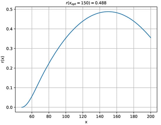
Figure 6.
Distribution of robustness of fertilizer doses x [kg/ha] to uncertain vegetation states of sugar beet cultivation determined with the numerical method.
Robustness distribution provides some interesting information. Only above the dose [kg/ha] there are such system states where the yield y [q/ha] can (but does not have to) enter the desired tolerance corridor [q/ha]. For smaller doses of fertilizer , only yields below 600 [q/ha] can be obtained. Above the dose , the number of states allowing to hit the tolerance corridor increases and reaches its maximum at the dose [kg/ha]. At this dose, the robustness to system uncertainty is 0.488. This means that with over 48% of possible states of the system, the yield will be in the range of [q/ha]. On the other hand, if one of the remaining 52% of possible states occurs in a given year, the desired yield will be not obtained.
Although the result [kg/ha] does not guarantee the desired yield , it is useful and realistic. There is no such dose x of fertilizer, which would guarantee a high yield in the range of [q/ha] under all possible growing conditions. If the growing conditions in the given year are critically unfavorable, e.g., very high temperatures, no rain at all, etc. it will not be possible to obtain high yields. Optimal fertilization promotes high yields, but does not guarantee them. This means that the problem under consideration does not have a tolerant solution in the sense of Shary’s definition [44]. There are no doses of fertilizer characterized by full (ideal) robustness . There are only fertilizer doses x that have a fractional (realistic) robustness.
The presented results (maximum fertilization robustness for ) were obtained by the numerical method and they can be not perfectly accurate. It seems that more accurate results can be obtained using the geometric calculation method. Figure 7 shows the full 3D-space of possible states of the vegetation system corresponding to the control value (decision variable) [kg/ha].
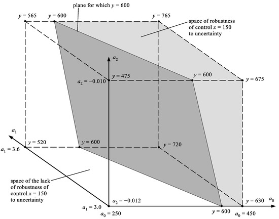
Figure 7.
Illustration of the geometric method of robustness calculating of fertilizer doses x [kg/ha]. is the full box volume of the possible states of the system, is the volume of the part of the box with the states guaranteeing the yield y lying in the tolerance corridor [q/ha].
At some points of the possible state box in Figure 7, the yield values y corresponding to these points are given. With the known control value , the value of the yield y is linearly dependent on values of the coefficients according to the equation of the system: . All points corresponding to the yield [q/ha] can be determined in the box. These points correspond to the plane crossing the state box shown in Figure 7. The shaded part of the box is the space with the volume , that is the space of states guaranteeing that the crop will hit the tolerance corridor . In the unshaded part of the box there are states that do not hit the tolerance corridor. After calculating the volume and (volume of the whole box), it is easy to calculate the robustness . This robustness is not much different from the robustness determined by the numerical method. Both methods indicate [kg/ha] as the optimal fertilization dose.
However, attention should be paid to the fact (Figure 6) that fertilization doses lower than also give high robustness to the uncertainty of the vegetation system. And so, the robustness for the dose [kg/ha] is , for the dose is , for the dose is , and for the dose the robustness , so almost exactly 0.4. This small decrease in robustness near the maximum makes it an attractive decision to reduce the fertilizer dose from optimal values of 150 to 140, 130, 120 or perhaps even 110 [kg/ha] because the cost of fertilizing the field will be significantly reduced taking into account the high prices of fertilizers. The decision to do so, however, depends on the decision-maker. i.e., the owner of the beet cultivation.
5. Determining the Roots of Interval Quadratic Equation
By solving the classic crisp quadratic Equation (35) with exactly known coefficients it is usually understood to find such values , for which the left side of the equation takes the value 0, Figure 8.
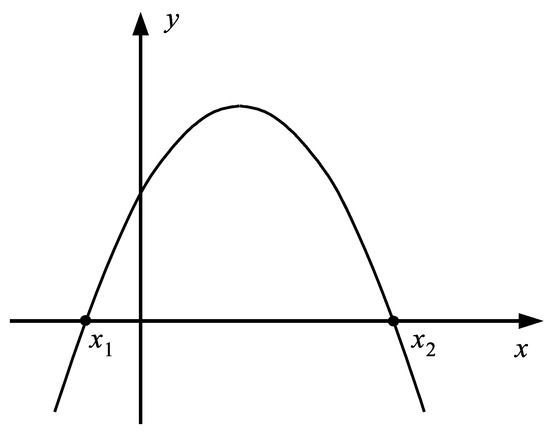
Figure 8.
Illustration of the sense of the roots , of the quadratic equation with exactly known values of the equation coefficients .
However, such an understanding of solving the quadratic equation is not always needed in practice. As an example, consider the fertilization equation for sugar beet (37).
Roots , of Equation (37) denote the amount of nitrogen fertilizer [kg/ha] that should be applied to obtain a zero yield y [q/ha]. This information is unlikely to interest the farmer. He is interested in possible yield increases. However, there are other problems in which the equation roots are useful. Therefore, in the following, we will show how to determine the roots of the interval quadratic equation using the example of Equation (37), in a purely mathematical sense.
Equation (37) can be interpreted as a tolerant control task in which the output y is required to be within the degenerate interval . Such a task can be solved mathematically using MIA. The solution is a set of pairs of roots conjugated by the RDM variables . However, none of the roots thus obtained has robustness to the uncertainty of the coefficients of Equation (37). Under the conditions of uncertainty of these coefficients, the chance of hitting by the left side of Equation (37) into the tolerance interval is infinitely small. In the case of the left side: , a realistic task is the task where the tolerance interval is not a degenerate zero but an extended zero [10]. Therefore, instead of (37), the problem (38) having a realistic tolerance range will be considered further.
Formula (38) after transfer into a multidimensional form with RDM variables takes the form (39) and after further transformations the form (40).
Note that the Equation (40) contains 5 variables—so it exists in the 5D space. The roots of Equation (40) can be calculated as:
Roots and are conjugated by the RDM variables. Only one pair of roots corresponds to one numerical combination of RDM variables . All combinations of allowed values of RDM variables allow the generation of all possible pairs of roots. Formula (41) also allow to determine the ranges (i.e., spans) of possible values of the roots and . Since these formulas are monotonic functions, their extrema appear on the borders of the domain. In order to determine these borders, it is enough to calculate the values of roots for all border combinations of RDM variables , i.e., for values 0 and 1. It is not a problem when using a computer. The results of this study are shown in (42).
Border values of the roots and were found for the following RDM variable values.
Equation (39) as a typical tolerant control equation was solved using the method given in Section 3 and Section 4. Figure 9 shows the domain of coupled pairs of roots .
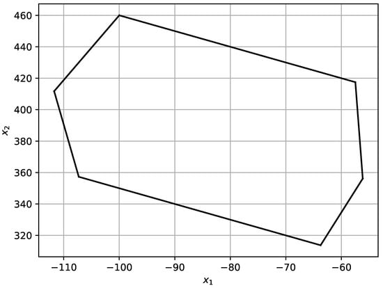
Figure 9.
Non-rectangular domain of conjugate pairs of roots of the tolerance Equation (39).
The spans of these roots given in (43) may suggest a rectangular domain. However, as shown in Figure 9, the actual domain is not a square one. The six characteristic border points of this domain correspond to 6 zero-one combinations of RDM variables. Each point inside the domain represents one pair of joined roots .
Figure 10 shows that it is difficult to hit the tolerance with both the root and the root . However, there is a realistic chance of that. The hitting difficulty is due to the small range of the assumed tolerance . However, it is more preferable to set as control value x one of the negative values of the optimal values of the root . They have the r value of the robustness which is greater than the most robust value of the root . This means that e.g., will hit the tolerance range if the true state of the uncertain control system will be one of about 10% of possible states, and not as in the case of using where the hit will be only for about 6% of possible states.
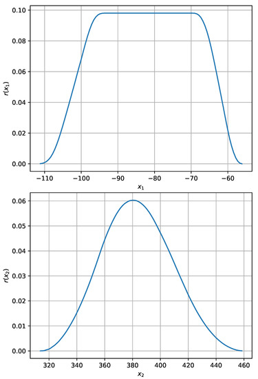
Figure 10.
Robustness distributions and of the roots of the quadratic tolerance Equation (39). The maximum robustness of the roots is different.
6. Conclusions
In the field of solving interval polynomial equations, including quadratic equations of the type (1), there is a research gap based on the fact that, in the case of many systems, the existing methods cannot find any physically feasible solution at all. There is a need to develop a method to fill this gap.
The article, after discussing the difficulties associated with solving quadratic interval equations, presents a method of finding solutions in the task of tolerant control of static systems in which the dependence of the output y on the input x (control, decision value) is quadratic. This method is illustrated by the example of the dependence of the yield y [q/ha] of a plant (sugar beet) on the dose x [kg/ha] of the applied fertilizer dose. The article shows that we often cannot obtain an ideal, tolerant solution x that guarantees the desired value of the controlled quantity (yield) . Usually we can only get a greater or lesser chance of an ideal solution. The reason for this state of affairs is the strong operation of many uncertainty generators, i.e., uncertain system parameters that we are not able to determine using measurement methods. The method shows, however, that there are better and worse solutions (controls) and that it is possible to define the optimal system control x which is robust to as many possible states of the uncertain system as possible. The realism of the presented method can be summarized as follows: although you are usually not able to control the real systems perfectly, that is, as we would like, the quality of our control can be increased to some extent thanks to the use of appropriate methods.
The scientific novelty of the method proposed in the paper is that it introduces for the first time the concept of robustness of a control value x to interval tolerance control systems. Robustness informs us at how many possible states of the uncertain system the given control x will meet the tolerance requirement. The second innovation of the method presented in the article is the dropping the idealistic requirement that the control value x should fulfill the task of hitting the tolerance corridor under all possible states of an uncertain system. This approach allowed the detection of the optimal control value that meets the tolerance task with as many possible system states as possible. The method presented in the article can be used in quadratic uncertain systems and, with minor modifications, in uncertain higher-order polynomial systems.
Author Contributions
Conceptualization, A.P.; methodology, A.P. and M.P.; software, M.P.; validation, A.P. and M.P.; formal analysis, A.P. and M.P.; investigation, A.P. and M.P.; resources, M.P.; data curation, M.P.; writing—original draft preparation, A.P. and M.P.; writing—review and editing, A.P. and M.P.; visualization, M.P.; supervision, A.P. All authors have read and agreed to the published version of the manuscript.
Funding
This research received no external funding.
Data Availability Statement
Not applicable.
Conflicts of Interest
The authors declare no conflict of interest.
Abbreviations
The following abbreviations are used in this manuscript:
| IA | interval arithmetic |
| IE | interval equation |
| FE | fuzzy equation |
| MIA | multidimensional interval arithmetic |
| SIA | standard interval arithmetic |
| RDM | relative distance measure |
| QIE | quadratic interval equation |
| QFE | quadratic fuzzy equation |
| SP | span |
| TC | tolerance corridor |
| UG | uncertainty generator |
References
- Ali, I.; Fügenschuh, A.; Gupta, S.; Modibbo, U. The LR-type fuzzy multi-objective vendor selection problem in supply chain management. Mathematics 2020, 8, 1621. [Google Scholar] [CrossRef]
- Rahman, M.S.; Shaikh, A.A.; Ali, I.; Bhunia, A.K.; Fügenschuh, A. A theoretical framework for optimality conditions of nonlinear type-2 interval-valued unconstrained and constrained optimization problems using type-2 interval order relations. Mathematics 2021, 9, 908. [Google Scholar] [CrossRef]
- Skorupa, A.; Piasecka-Belkhayat, A. Numerical modeling of heat and mass transfer during cryopreservation using interval analysis. Appl. Sci. 2020, 11, 302. [Google Scholar] [CrossRef]
- Zheng, Z.; Xie, Y.; Zhang, D. Numerical investigation on the gravity response of a two-pole generator rotor system with interval uncertainties. Appl. Sci. 2019, 9, 3036. [Google Scholar] [CrossRef]
- Piegat, A.; Pluciński, M. The optimal tolerance solution of the basic interval linear equation and the explanation of the Lodwick’s anomaly. Appl. Sci. 2022, 12, 4382. [Google Scholar] [CrossRef]
- Oettli, W.; Prager, W. Compatibility of approximate solution of linear equations with given error bounds for coefficients and right-hand sides. Numer. Math. 1964, 6, 405–409. [Google Scholar] [CrossRef]
- Oettli, W. On the solution set of a linear system with inaccurate coefficients. J. Soc. Ind. Appl. Math. Ser. B Numer. Anal. 1965, 2, 115–118. [Google Scholar] [CrossRef]
- Gay, D. Solving linear interval equations. SIAM J. Numer. Anal. 1982, 19, 858–870. [Google Scholar] [CrossRef]
- Lodwick, W.; Dubois, D. Interval linear systems as a necessary step in fuzzy linear systems. Fuzzy Sets Syst. 2015, 281, 227–251. [Google Scholar] [CrossRef]
- Dymova, L.; Sevastjanov, P.; Pownuk, A.; Kreinovich, V. Practical need for algebraic (equality-type) solutions of interval equations and for extended-zero solutions. In Proceedings of the International Conference on Parallel Processing and Applied Mathematics, Lublin, Poland, 10–13 September 2017; Springer: Berlin/Heidelberg, Germany, 2017; pp. 412–421. [Google Scholar]
- Sevastjanov, P.; Dymova, L. A new method for solving interval and fuzzy equations: Linear case. Inf. Sci. 2009, 179, 925–937. [Google Scholar] [CrossRef]
- Buckley, J.; Qu, Y. Solving linear and quadratic fuzzy equations. Fuzzy Sets Syst. 1990, 38, 43–59. [Google Scholar] [CrossRef]
- Buckley, J.; Qu, Y. Solving fuzzy equations: A new solution concept. Fuzzy Sets Syst. 1991, 39, 291–301. [Google Scholar] [CrossRef]
- Buckley, J.; Qu, Y. Solving systems of linear fuzzy equations. Fuzzy Sets Syst. 1991, 43, 33–43. [Google Scholar] [CrossRef]
- Buckley, J. Solving fuzzy equations. Fuzzy Sets Syst. 1992, 50, 1–14. [Google Scholar] [CrossRef]
- Barth, W.; Nuding, E. Optimale lösung von intervallgleichungssystemen. Computing 1974, 12, 117–125. [Google Scholar] [CrossRef]
- Dymova, L.; Sevastjanov, P. A new method for solving nonlinear interval and fuzzy equations. In Proceedings of the International Conference on Parallel Processing and Applied Mathematics, Lublin, Poland, 10–13 September 2017; Springer: Berlin/Heidelberg, Germany, 2017; pp. 371–380. [Google Scholar]
- Allahviranloo, T.; Gerami Moazam, L. The solution of fully fuzzy quadratic equation based on optimization theory. Sci. World J. 2014, 156203. [Google Scholar] [CrossRef]
- Allahviranloo, T.; Ghanbari, M. On the algebraic solution of fuzzy linear systems based on interval theory. Appl. Math. Model. 2012, 36, 5360–5379. [Google Scholar] [CrossRef]
- Allahviranloo, T.; Ghanbari, M.; Hosseinzadeh, A.; Haghi, E.; Nuraei, R. A note on “Fuzzy linear systems”. Fuzzy Sets Syst. 2011, 177, 87–92. [Google Scholar] [CrossRef]
- Friedman, M.; Ming, M.; Kandel, A. Fuzzy linear systems. Fuzzy Sets Syst. 1998, 96, 201–209. [Google Scholar] [CrossRef]
- Kreinovich, V. Solving equations (and systems of equations) under uncertainty: How different practical problems lead to different mathematical and computational formulations. Granul. Comput. 2016, 1, 171–179. [Google Scholar] [CrossRef]
- Landowski, M. RDM interval method for solving quadratic interval equation. Przegląd Elektrotechniczny 2017, 93, 65–68. [Google Scholar] [CrossRef][Green Version]
- Hasan, M.; Badsha, M.; Sobhan, M. A different approach to solve fuzzy quadratic equation AX2 = B. IOSR J. Eng. 2019, 9, 1–7. [Google Scholar]
- Buckley, J.; Jowers, L. Solving fuzzy equations. In Monte Carlo Methods in Fuzzy Optimization; Springer: Berlin/Heidelberg, Germany, 2007; pp. 89–115. [Google Scholar]
- Hong, D. On solving fuzzy equation. Korean J. Comput. Appl. Math. Ser. A 2001, 8, 213–224. [Google Scholar]
- Bhiwani, R.; Patre, B. Solving first order fuzzy equations: A modal interval approach. In Proceedings of the Second International Conference on Emerging Trends and Technology ICETET-09, Nagpur, India, 16–18 December 2009; IEEE Computer Society: Washington, DC, USA, 2009; pp. 953–956. [Google Scholar]
- Ahmad, M.; Jamaluddin, N.; Sakib, E.; Daud, W.; Aswad, N.; Rahman, A. Fuzzy false position method for solving fuzzy nonlinear equations. ARPN J. Eng. Appl. Sci. 2016, 11, 9737–9745. [Google Scholar]
- Sulaiman, I.; Mamat, M.; Mohamed, M.; Waziri, M. Diagonal updating Shamanskii-like method for solving singular fuzzy nonlinear equations. Far East J. Math. Sci. 2018, 103, 1619–1629. [Google Scholar] [CrossRef]
- Sulaiman, I.; Mamat, M.; Waziri, M.; Mohamed, M.; Mohamad, F. Solving fuzzy nonlinear equation via Levenberg-Marquardt method. Far East J. Math. Sci. 2018, 103, 1547–1558. [Google Scholar] [CrossRef]
- Omesa, U.; Mamat, M.; Sulaiman, I.; Sukono, S. On quasi Newton method for solving fuzzy nonlinear equations. Int. J. Quant. Res. Model. 2020, 1, 1–10. [Google Scholar] [CrossRef]
- Sulaiman, I.; Mamat, M.; Waziri, M.; Fadhilah, A.; Kamfa, K. Regula Falsi method for solving fuzzy nonlinear equation. Far East J. Math. Sci. 2016, 100, 873–884. [Google Scholar] [CrossRef]
- Sulaiman, I.; Mamat, M.; Ghazali, P. Shamanskii method for solving parameterized fuzzy nonlinear equations. Int. J. Optim. Control Theor. Appl. 2021, 11, 24–29. [Google Scholar]
- Sulaiman, I.; Mamat, M.; Nurnadiah, Z.; Puspa, L. Solving dual fuzzy nonlinear equations via Shamanskii method. Int. J. Eng. Technol. 2018, 7, 89–91. [Google Scholar] [CrossRef]
- Kajani, M.; Asady, B.; Vencheh, A. An iterative method for solving dual fuzzy nonlinear equations. Appl. Math. Comput. 2005, 167, 316–323. [Google Scholar] [CrossRef]
- Jun, Y. Tri-section method for solving fuzzy non-linear equations. Int. J. Sci. Innov. Math. Res. 2019, 7, 4–7. [Google Scholar]
- Nieto, J.J.; Rodríguez-López, R. Existence of extremal solutions for quadratic fuzzy equations. Fixed Point Theory Appl. 2005, 3, 1–22. [Google Scholar] [CrossRef]
- Khan, N.; Yaqoob, N.; Shams, M.; Gaba, Y.U.; Riaz, M. Solution of linear and quadratic equations based on triangular linear diophantine fuzzy numbers. J. Funct. Spaces 2021, 8475863. [Google Scholar] [CrossRef]
- Mamehrashi, K. A new method for solving interval and fuzzy quadratic equations of dual form. UKH J. Sci. Eng. 2021, 5, 81–89. [Google Scholar] [CrossRef]
- Xu, D.; Wang, Q.; Li, Y. Adaptive optimal robust control for uncertain nonlinear systems using neural network approximation in policy iteration. Appl. Sci. 2021, 11, 2312. [Google Scholar] [CrossRef]
- Piegat, A.; Pluciński, M. Inclusion principle of fuzzy arithmetic results. J. Intell. Fuzzy Syst. 2022, 42, 4987–4998. [Google Scholar] [CrossRef]
- Shary, S. Optimal solution of interval linear algebraic systems. Interval Comput. 1991, 2, 7–30. [Google Scholar]
- Shary, S. On controlled solution set of interval algebraic systems. Interval Comput. 1992, 6, 66–75. [Google Scholar]
- Shary, S. Solving the tolerance problem for interval linear systems. Interval Comput. 1994, 2, 6–26. [Google Scholar]
- Boukezzoula, R.; Foulloy, L.; Coquin, D.; Galichet, S. Gradual interval arithmetic and fuzzy interval arithmetic. Granul. Comput. 2019, 6, 451–471. [Google Scholar] [CrossRef]
- Piegat, A.; Landowski, M. Is the conventional interval-arithmetic correct? J. Theor. Appl. Comput. Sci. 2012, 6, 27–44. [Google Scholar]
- Piegat, A.; Tomaszewska, K. Decision-making under uncertainty using Info-Gap Theory and a new multidimensional RDM interval-arithmetic. Przegląd Elektrotechniczny 2013, 89, 71–76. [Google Scholar]
- Piegat, A.; Landowski, M. Multidimensional approach to interval-uncertainty calculations. In New Trends in Fuzzy Sets, Intuitionistic Fuzzy Sets, Generalized Nets and Related Topics, Vol. II: Applications; System Research Institute of Polish Academy of Sciences: Warsaw, Poland, 2013; pp. 137–152. [Google Scholar]
- Piegat, A.; Landowski, M. Two interpretations of multidimensional RDM interval arithmetic: Multiplication and division. Int. J. Fuzzy Syst. 2013, 15, 486–496. [Google Scholar]
- Piegat, A.; Pluciński, M. Some advantages of the RDM-arithmetic of Intervally-Precisiated Values. Int. J. Comput. Intell. Syst. 2015, 8, 1192–1209. [Google Scholar] [CrossRef][Green Version]


Publisher’s Note: MDPI stays neutral with regard to jurisdictional claims in published maps and institutional affiliations. |
© 2022 by the authors. Licensee MDPI, Basel, Switzerland. This article is an open access article distributed under the terms and conditions of the Creative Commons Attribution (CC BY) license (https://creativecommons.org/licenses/by/4.0/).