Abstract
Since the emergence of artificial intelligence and deep learning methods, the fault diagnosis of bearings in rotating machinery has gradually been realized, reducing the high costs of bearing faults. However, in the actual work of the equipment, faults rarely occur, resulting in less fault data. Therefore, it is necessary to study small sample fault data. For the case of less fault data, the Maml–Triplet fault classification learning framework based on the combination of maml and the triplet neural network is proposed. In the framework of Maml-Triplet fault classification, firstly, an initial signal feature extractor is obtained using the Maml training method. Secondly, the feature vectors corresponding to signal data are obtained using depth distance measurement learning in the triplet neural network, and the fault type is judged based on the feature vectors of unknown signal. The results show that the accuracy of the Maml–Triplet model is 2% higher than that of the triplet model alone and 5% higher than that of the Maml–CNN meta learning method. When there are fewer data samples, the accuracy gap is more obvious. Therefore, in the case of less data, the Maml–Triplet model has an excellent fault identification ability.
1. Introduction
Rotating equipment is an important part of many mechanical systems and bearings are widely used. When the fault occurs, if the fault type can be judged in time, it can provide important support for maintenance decision-making. It can make up for the economic losses caused by equipment outage owing to failure to the maximum extent. At present, fault diagnosis technology is widely used in manufacturing, the aviation industry, automobile, power generation, transportation, and other fields [1,2,3], and has led to great achievements.
With the rapid development of artificial intelligence methods such as deep learning in computer vision, image and video processing, speech recognition, and other application fields [4], deep learning methods are gradually applied to fault diagnosis. Compared with traditional fault diagnosis technology, intelligent fault diagnosis technology based on deep learning has the advantages of high reliability and efficiency, so it has attracted widespread attention and application in the academic community [5]. High level achievements have been achieved in fault diagnosis using an automatic encoder (AE) [6,7,8,9], restricted Boltzmann machine (RBM) [10,11,12], convolutional neural network (CNN) [13,14,15,16], recurrent neural network (RNN) [17,18], neural network based migration learning [19,20], and generative countermeasures networks (GANs) [21].
For example, Sun combined a sparse automatic encoder with deep belief network and proposed the SAE-DBN neural network for bearing fault diagnosis to achieve excellent feature learning and classification performance [7]. Gao achieved an aircraft fuel system failure diagnosis using a deep quantum inspired neural network (DQINN) [11]. Li et al. proposed IDSCNN, based on ensemble deep convolutional neural networks and an improved Dempster–Shafer theory, for bearing fault diagnosis, whose input is an FFT feature of the vibration signals from two sensors [14]. Zhao et al. designed a deep neural network structure called convolutional bidirectional long short-term memory (CBLSTM) to process raw sensory data [17]. In order to solve various operating conditions in fault diagnosis, Shao et al. proposed a fault diagnosis method based on migration learning [8]. Yang et al. proposed a feature-based transfer neural network (FTNN) [22].
However, the following phenomena exist in the actual work of the equipment: first, the equipment is not allowed to fail, especially the key systems and key failures; second, most failures occur slowly and equipment failures may occur for months or years; and third, the working conditions of the mechanical system of the equipment are very complex and the production requirements are often changed. It is unrealistic to collect and mark sufficient training data. These phenomena lead to insufficient data for deep neural network learning in practical work.
For small sample learning fault diagnosis technology, in addition to data enhancement technology, another promising method to alleviate the problem of limited data is a small amount or one-time learning method [10], which has been successfully applied to a variety of tasks, including a small amount of image recognition, path planning of artificial intelligence, and recent fault diagnosis [23]. The few shot learning model has a strong generalization ability for categories with only a few samples in the training process [24]. It includes the maml learning method, Siamese network [25], and triplet neural network.
Chelsea Finn et al. proposed the maml meta training learning method. In addition to more effectively summarizing new tasks, maml can also learn the process of learning itself, that is, how to learn [26]. As shown in Figure 1 and Figure 2, Maml uses quadratic gradient iteration to descend and find a group of weight parameters with higher sensitivity. For multiple tasks, it can achieve global optimization through a few gradient iterations.
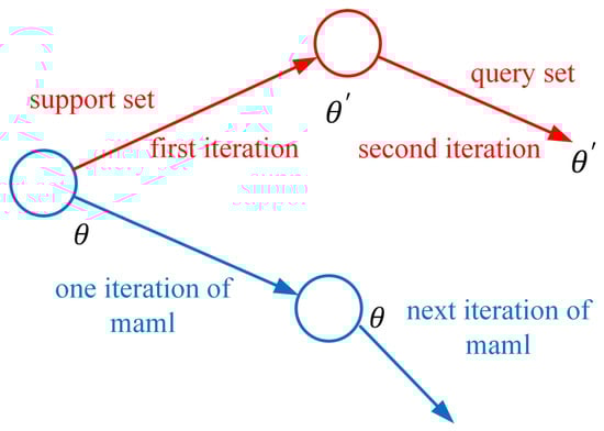
Figure 1.
Maml quadratic gradient iteration process.
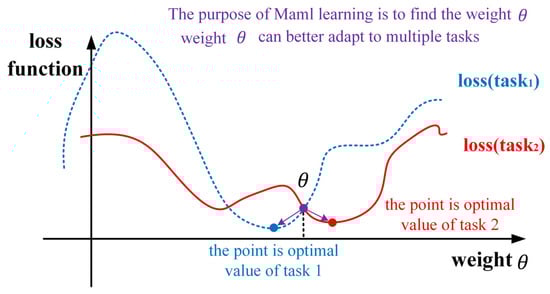
Figure 2.
Initial weights for multitasking.
Liu X et al. created the mamb model according to the maml model, randomly selected some data from the training set to form multiple fault classification tasks for training the maml model, and fine-tuned the following model layers at a low learning rate to obtain the final mamb model [27]. Zhang S et al. proposed a bearing fault diagnosis model based on the maml model for small sample learning. The experimental results show that the accuracy of the twin neural network is 25% higher than that of the twin neural network [28]. Yang TY et al. proposed a new maml cross domain fault diagnosis method to improve the performance of the model by adding data from other working conditions or other datasets [29]. Dixit et al. proposed a new conditional auxiliary classifier GAN framework with the MAML meta learning method, which has good performance for finite datasets [30].
Hermans et al. used triplet loss function to model the details of input pictures and learned a better classification method for input pictures by comparing the distance measurement difference between the same type of pictures and different types of data pictures [31]. As shown in Figure 3, the triplet neural network is mainly used to train samples with small differences. Wang et al. proposed a countermeasure domain adaptive method based on triplet loss function guidance for bearing fault diagnosis [32]. Zhang K et al. proposed a triplet triple metric driven multi head graph neural network to enhance the identification of unknown signals through decoupling confrontation learning [33]. For classification of small sample rolling bearing fault datasets, Yang et al. propose a coupling vibration data classification method based on triplet embedding [34].
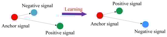
Figure 3.
Learning process of the triplet neural network.
Both the maml meta learning method and triplet depth metric learning method show good results for small sample learning. We consider that the maml meta learning method can quickly create new classification tasks, but it may not be able to obtain the optimal results. Triplet depth metric learning has a good classification effect on small sample data, but it needs to judge difficult triples in the training process, resulting in the problem of a long training time. We created the maml triplet learning method, drawing on the rapid adaptability of the maml meta learning method and the excellent small sample classification effect of the triplet depth metric learning method. The specific improvement methods are as follows:
- The Maml–Triplet model for small sample fault diagnosis is proposed. An initial feature extractor that can be quickly adapted to multiple fault classification tasks is obtained using the Maml meta learning method, then the feature vector of signal is obtained using triplet depth measurement learning, and the fault type of unknown signal is judged by comparing the Euclidean distance of the feature vectors between different signals.
- In the experiment, two datasets for training the Maml neural network are constructed using three-way five-shot fault classification tasks and three-way ten-shot fault classification tasks. Moreover, two different maml-triplet models are constructed based on two different Maml models. Finally, it is proved through experiments that the results of the two Maml–Triplet models are better than those of the other models with different numbers of datasets.
- The influence of the number of fault types and the number of signal data in a single fault on the accuracy of the model is studied. Experiments show that, the more fault types, the lower the accuracy; the less signal data in a single fault, the lower the accuracy. In the experiment, it is also found that the number of fault types and the number of signal data within a single fault have less influence on the Maml–Triplet model than other models.
2. Maml–Triplet Learning Method
As the probability of failure in the actual work of the equipment is small, a Maml–Triplet method is proposed, which aims to use the original fault dataset to gain the ability to quickly learn new small sample fault data. In this paper, the original fault dataset is called the source domain data set and the small sample fault dataset that needs to be identified quickly is called the target domain dataset. The Maml–Triplet learning method uses the maml meta learning method to learn the parameters of the neural network in the source domain dataset and prepare for the triplet neural network to quickly adapt to the target domain dataset. Under the Maml–Triplet training framework, the weight update process is shown in Figure 4. The maml triplet learning framework includes two parts: maml neural network and triplet neural network. First, the initial weights are obtained using the maml meta learning method. Similarly, through similar transfer learning, the training weights in the maml neural network are assigned to the triplet neural network. According to the triplet loss function, the triplet neural network is trained. Finally, the triplet neural network is still used to identify unknown signals.
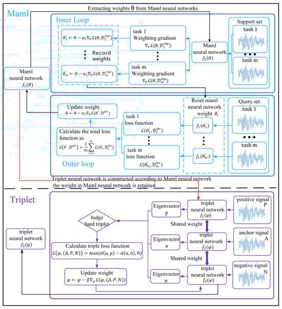
Figure 4.
Weight update process under the Maml–Triplet training framework.
2.1. Maml Meta Learning Method
In the standard supervised learning, as shown in Formula (1), the function of deep learning is to obtain the function f that maps an input data x, such as a signal, to the corresponding fault tag y of the signal. In the supervised meta learning method, the idea is very similar. According to a dataset , which includes multiple fault classification tasks, a function F is found, as shown in Formula (2). Its function is to find a function f that maps the input signal data to the fault tag in the standard supervised learning. In other words, the supervised meta learning method aims to find a function F with the ability to find the function f according to the dataset. The Maml learning method is one of the meta learning methods.
The role of the Maml meta learning method in the Maml–Triplet method is to obtain a model in the source dataset that can be quickly applied to a few shot task. The Maml meta learning method obtains a better initial value of the model through preliminary training. Then, based on the initial weights, a small amount of update weights for specific small sample training data tasks can achieve better results. It can be understood as searching for a group of weight parameters with high sensitivity. Based on these highly sensitive weight parameters, ideal results can be achieved in new small sample tasks with only a small number of iterations.
As shown in Figure 4, the neural network composed of weights can be divided into the inner loop and outer loop in the process of maml meta learning training. In the inner loop process, when adapting to new tasks , the neural network uses the cross entropy loss function for each classification task and uses the gradient descent method to update the neural network weight to the weight , as shown in Formulas (3) and (4). Note that the weight update process occurs in each classification task and does not change the weight parameters of the external network model.
is a classification task in the support set dataset; is a pair of input and output data in ; and is the super parameter inner loop learning rate.
During the outer loop process, the weight of the neural network needs to be reset for each classification task as follows: . For each classification task , the cross entropy loss function is still selected as shown in Formulas (5)–(7), and the gradient descent method is used to update the neural network weight . At this point, an iteration is completed.
is a classification task in the query set dataset; is a pair of input and output data in ; and is the super parameter outer loop learning rate.
2.2. Depth Metric Learning Method Based on Triplet Loss Function
For the fault classification task with more categories and less data in the category, the depth metric learning method based on triple loss function can effectively solve this problem. First, the triplet neural network is constructed according to the trained Maml neural network , and the triplet neural network weights are initialized using the trained Maml neural network weight . Then, the triplet is selected to build the input data, including anchor example A, positive example P, and negative example N. The positive example is a signal of the same category as the anchor example, and the negative example is a signal of a different category from the anchor example. The triplet neural network is used to map the triplet signal into three eigenvectors, namely, anchor example eigenvector a, positive example eigenvector p, and negative example eigenvector n. The triplet loss function is defined according to the Euclidean distance between the triplet eigenvectors, as shown in Formulas (8) and (9).
where , , . represents the euclidean distance between the anchor example feature vector and the positive example feature vector and represents the Euclidean distance between the anchor example feature vector and the negative example feature vector, and maximum spacing .
Then, the gradient descent method is used to update the weight . As shown in Formula (10), is the super parameter learning rate.
If all of the samples in the training set participate in the construction of triples, then the number of triples is very large and there are a large number of triples with their own loss function of 0. These triples will cause slow convergence of the model and the characteristics do not have uniqueness. Therefore, it is necessary to select the triad that is meaningful for training, that is, in each training iteration, the difficult triad is selected according to Formula (11).
Next, the process of diagnosing unknown fault signals after training the triplet neural network is introduced. The n-way k-shot is taken as an example. First, as shown in Formulas (12) and (13), a template library is constructed based on the signal data in the training set. That is, the triplet neural network is used to extract eigenvectors for all signals of the same fault type and the average value of all eigenvectors is taken. Secondly, the triplet neural network is used to extract the eigenvectors of unknown signals and the eigenvectors in the template library are used to measure the Euclidean distance. Finally, as shown in Formula (14), various Euclidean distances are compared to find the feature vector with the minimum distance from the unknown signal feature vector in the template library , and the corresponding fault type is the fault type of the unknown signal.
where X represents the input signal data, represents the eigenvector of the j-th fault type, x represents unknown data, and represents the template library.
3. Construction of the Dataset and Model
3.1. Dataset Introduction
The CWRU bearing dataset [35] is adopted in this paper. The test bed is composed of a motor, torque sensor/encoder, dynamometer, and control electronic equipment. The test bearing is installed at the fan end and motor end. A single point fault was introduced into the test bearing using the method of electrical discharge machining. The diameter of the fault was 0.007 inches, 0.014 inches, and 0.021 inches, respectively. The fault points are located in the inner raceway, rolling element, and outer raceway of the bearing. The accelerometer used to detect the vibration signal is installed at the 12 o’clock position of the fan end and motor end of the motor housing, and some experiments are also installed on the motor support substrate. During the experiment, the vibration data generated under the load of 0 to 3 horsepower motor were recorded, and 12,000 data were collected per second. For more details on the CWRU bearing dataset, please visit its website [36].
This paper selects the data generated by the fan end bearing as the source dataset and the data generated by the motor end bearing as the target data set. The experimental conditions are all no-load. There are three fault locations and three types of faults for the selected test bearings. As shown in Table 1 and Table 2, Group A signals are source data sets, with a total of nine categories; Group B signals are target datasets and there are nine categories in total. Table 3 shows the frequency of its failures.

Table 1.
Fault categories of the source dataset.
Table 2.
Fault categories of the target dataset.
Table 3.
Bearing fault frequencies. BPFI: ball pass frequency, inner race; BPFO: ball pass frequency, outer race; FTF: fundamental train frequency (cage speed); BSF: ball (roller) spin frequency.
3.2. Data Preprocessing
The dataset selected in this paper is the vibration signals measured at different parts of the motor. These signals cannot be trained directly and need to be processed by preprocessing methods.
Experimental data were collected at 12,000 samples/second and motor speeds of 1797 to 1720 RPM. It can be calculated that 400–418 samples are collected when the shaft rotates for one circle. As shown in Table 3, the fault frequencies BPFI, BPFO, and BSF are greater than the rotation frequency of the shaft, so a cycle can be covered by collecting fewer points. The more points selected, the higher the accuracy of the model prediction, but the higher the training cost. In this paper, 2048 points are sampled as one input data, which includes all bearing fault cycles and has good performance.
As shown in Figure 5, first, the multi-source signal fusion method is used to sample the original vibration signals measured at the fan end and motor end at the same time and the signal length of 2048 is intercepted to form an array with the shape of (2048, 2). For example, as shown in Formulas (15)–(17), the fan end signal and motor end signal are selected with a length of 2048 at the same time and and are combined into matrix . Secondly, after the normalization processing of Formula (18), signal data available for use are obtained. After that, on the basis of data preprocessing, the datasets of Maml neural network and Triplet neural network are constructed.
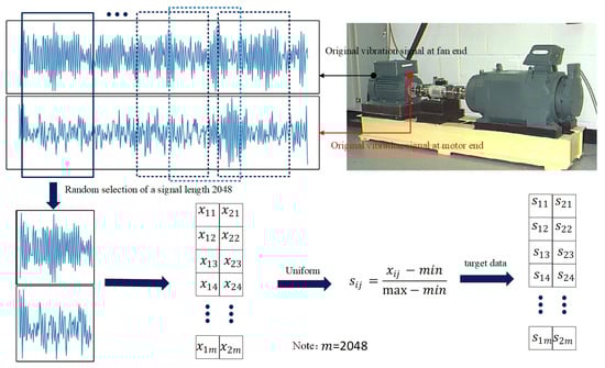
Figure 5.
Processing process of bearing fault signal.
3.3. Construction Method of the Maml Neural Network Dataset and Triplet Neural Network Data
As shown in Table 1 and Table 2, the dataset for training the maml neural network is constructed using Group A signals. The data used by the maml neural network are no longer a single signal, but the fault classification task is used as the input data. The n-way k-shot model is taken as an example, that is, n fault types and k signal data in each type as an example. Firstly, n fault types are randomly selected from nine signal types of Group A signal. According to the above data preprocessing method, k signals are randomly intercepted from a fault type. After the order is disturbed, an n-way k-shot fault classification task is generated. The above operations are repeated to generate multiple fault classification tasks and to form a dataset of the Maml neural network.
A dataset is built for training the triplet neural network based on Group B signals. At each input signal, three signals are simultaneously selected as a triplet, which are positive examples, anchor examples, and negative examples. In the training process, after each weight update, the eigenvectors of the three signals are calculated respectively according to the updated Triplet neural network, and the difficult triplets are selected according to the Euclidean distance between the characteristic signals. Note that the triplet neural network dataset is not created at the beginning of the training, but is updated and selected to form a new dataset during the network training.
3.4. Construction Method of the Maml Neural Network and Triplet Neural Network Model
In the Maml–Triplet model, there are two parts: the maml neural network and the triplet neural network. The structure of the maml neural network and the triplet neural network is shown in the Figure 6. The triplet neural network is a part of the secondary maml neural network.
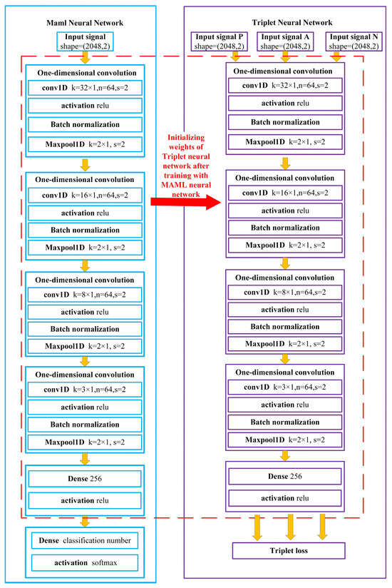
Figure 6.
Network structure of the maml neural network and triplet neural network.
As shown in Figure 6, the triplet neural network is composed of four convolution blocks and a full connection layer. The convolution block is composed of a convolution layer, pooling layer, and batch normalization layer. Among the four convolution blocks, only the convolution layer is different. The parameters of the first convolutional layer include 64 convolution kernels of size 32 × 1 with stride 2. The parameters of the second convolution layer include 64 convolution kernels of size 16 × 1 with stride 2. The parameters of the third convolution layer include 64 convolution kernels of size 8 × 1 with stride 2. Finally, the parameters of the fourth convolution layer include 64 convolution kernels of size 3 × 1 with stride 2. The pooling layer adopts the maximum pooling with a size of 2 and a step size of 2. The last layer is a fully connected layer with 256 nodes, which is used to transform signals into 256 dimensional eigenvectors.
The maml neural network structure adds a full connection layer with Softmax activation function on the basis of the triplet neural network structure. The number of nodes is the total number of fault types included in each task during the training process of Maml. This paper sets the number of nodes as 3. The activation functions of the remaining layers are set to ReLU.
The network structure of the comparison experiment Maml–CNN modifies the number of nodes in the last layer of the Maml neural network according to the number of fault types in the data set. The training process also extracts the weight of the Maml neural network and then uses the target dataset for training to obtain the final model.
It should be noted here that, as shown in Figure 5, the initial weight of the triplet neural network is the neural network trained by the Maml neural network. In the subsequent training, the weight is updated at a lower learning rate.
4. Experimental Process and Results
4.1. Experimental Process and Results of the Maml Learning Method
To prevent experimental specificity, two models of three-way five-shot and three-way ten-shot were constructed using a dataset during Maml–Triplet training. According to the construction method of the Maml model, 25 fault classification tasks are created in Group A data as the support set dataset for the inner loop in the Maml training process, and 25 fault classification tasks are also created as the query set data set for the outer loop in the Maml training process.
After many experiments, the gradient descent method of Adam is selected for the inner loop and the learning rate of the inner loop is set to 0.1. The gradient descent method of Adam is used for the outer loop and the learning rate of the outer loop is set to 0.01. After 1000 iterations, the weight of the minimum loss function is selected to prepare the Maml–Triplet model. The accuracy and loss functions during Maml training are shown in Figure 7 and Figure 8. The three-way ten-shot model is better than the three-way five-shot model.
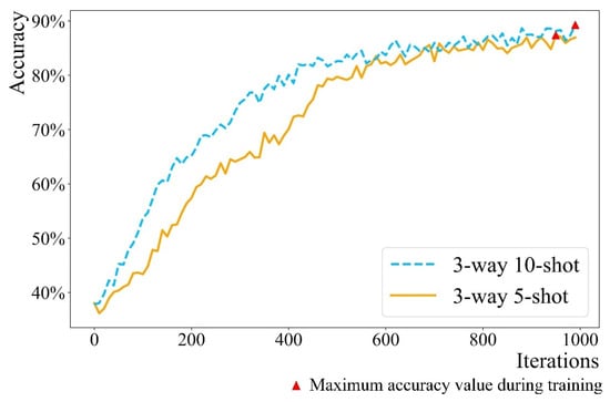
Figure 7.
Trend chart of accuracy during Maml training.
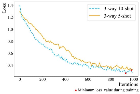
Figure 8.
Trend chart of loss function during Maml training.
4.2. Test Criteria for Models
Because of the small sample learning, in order to test the reliability of the model, more samples are selected during the test, i.e., 200 signal data are selected for each fault category. The experimental process is as follows. Taking n-way k-shot as an example, n fault types are randomly selected from the target dataset and each type has k training sets of signal data. A test set of n-way 200-shot is created in a similar way. Then, different learning methods are chosen to use training sets for training and test sets for testing. Five repeated experiments from dataset creation to training model were conducted, and the average accuracy of the five test sets was used as a measure of the quality of each learning method.
4.3. Experimental Process and Results of the Maml–Triplet Learning Method
The triplet neural network structure is constructed using the methods mentioned above, the triplet dataset is constructed using Group B data in each iteration, and the neural network weights of the completed three-way five-shot and three-way ten-shot Maml models are extracted to construct the Maml–Triplet learning models of Maml5–Triplet and Maml10–Triplet. Next, the triplet neural network part is trained. During the training process, the Adam gradient descent method is used, the learning rate is set to 0.001, and the maximum interval of the triplet loss function is set to 0.5. In the experiment, the Maml–Triplet learning method is compared with Triplet, CNN, and Maml–CNN learning methods. The effects of the number of fault types and the number of signals in a single fault type on each learning method are studied respectively.
4.3.1. Research on the Effect of the Number of Failure Types on Different Learning Methods
When studying the effect of fault type quantity on different models, under the condition of signal quantity in the same single fault type, six classification tasks from three-way to nine-way are designed, that is, the number of fault types ranges from six to nine. As shown in Figure 9, Figure 10 and Figure 11, there are three groups of experiments: 5-shot, 10-shot, and 15-shot. Each fault type has 5, 10, and 15 signals, respectively. In general, the accuracy of Maml5–Triplet and Maml10–Triplet models is higher than that of the triplet, Maml–CNN, Siamese, and CNN models. Especially when there are five signal data for each fault type, the Maml–Triplet model is obviously superior to other models.
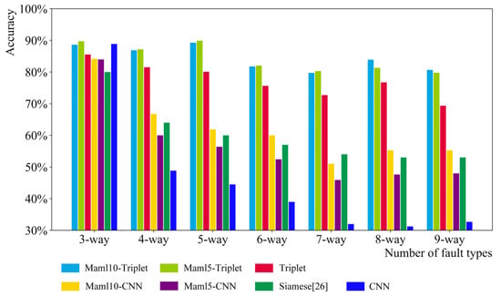
Figure 9.
n-way five-shot classification result.
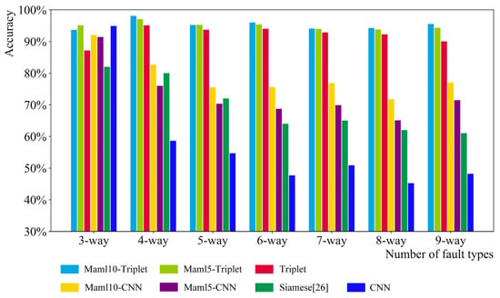
Figure 10.
n-way 10-shot classification result.
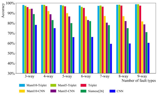
Figure 11.
n-way 15-shot classification result.
The accuracy of the Maml–Triplet model and the triplet model fluctuates when the number of samples is small, i.e., five signal data for each fault type. When each fault type contains 10 signal data and 15 signal data, the accuracy of Maml–Triplet model is about 95% and 98%, respectively, which is about 2% higher than that of the triplet model. However, with the increase in fault types, the accuracy of the Siamese, Maml–CNN, and CNN models decreases gradually, especially the CNN model. However, the number of fault types is between three and nine, and the increase in fault types has little effect on the Maml–Triplet model.
4.3.2. Research on the Influence of the Number of Signals in a Single Fault on Different Learning Methods
When studying the effect of signal quantity in a single fault type on different models, under the same fault type quantity condition, the average accuracy on the test set after five training sessions of different models is designed under six fault classification tasks of 5, 10, 15, and 25 signals in a single fault type. As shown in Figure 12 and Figure 13, there are two groups of experiments, that is, the number of fault types is 4 and 10.
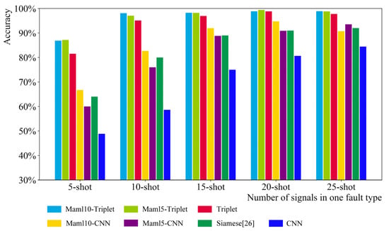
Figure 12.
Four-way k-shot classification result.
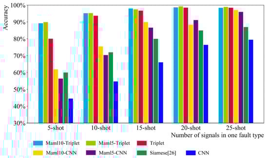
Figure 13.
Five-way k-shot classification result.
The experimental results show that the accuracy of the Maml–Triplet model increases with the number of fault signals. When the number of fault signals reaches 20, the accuracy of the Maml–Triplet model reaches the maximum of about 99% and tends to be stable. The accuracy of the Maml–Triplet model is significantly higher than that of the other three models when the number of fault signals is at least five. Compared with the Siamese, Maml–CNN, and CNN model, the Maml–Triplet model can better identify faults with less data.
5. Conclusions and Prospect
This paper aims at the low frequency of faults during equipment operation and the small amount of fault data that is not easy to cause by collecting fault signals. A small sample-bearing fault diagnosis framework based on the Maml–Triplet model is proposed, and the validity of the proposed framework in identifying new artificial bearing faults is verified using CWRU datasets.
When the Maml–Triplet model has 20 samples in each fault type, its accuracy can reach about 99% and its effect is better than that of the triplet model, Maml–CNN model, and CNN model. When there are less than 20 samples per fault type, the accuracy of the Maml–Triplet model increases with the number of samples. Furthermore, when increasing the number of fault types, the accuracy of the Maml–Triplet model is relatively stable, which is significantly better than that of the Maml–CNN model and CNN model. In conclusion, the Maml–Triplet model is significantly superior to other models under small sample conditions.
Of course, there are still some shortcomings in the Maml–Triplet model. For example, during the training of the Maml neural network, there are disadvantages such as an unstable secondary gradient and slow training speed. For the MAML training process, Antoniou et al. proposed an improved method in the literature [37]. The Maml–Triplet model can only be used for supervisory tasks, but it cannot process data without a label or with an incomplete label and cannot use the signal without a label at the early stage of equipment, which results in a certain degree of data waste.
Future work will study semi-supervised learning in the case of small sample data and missing labels based on the maml meta learning method
Author Contributions
Conceptualization, Q.C.; Data curation, Z.H.; Formal analysis, Z.H.; Funding acquisition, Q.C. and Z.Z.; Methodology, Z.H.; Project administration, Z.L.; Resources, Q.C. and Z.Z.; Software, Z.H. and Z.Z.; Supervision, Z.L.; Validation, Y.L.; Visualization, Y.L.; Writing—original draft, T.Z.; Writing—review and editing, T.Z. All authors have read and agreed to the published version of the manuscript.
Funding
This research is supported by JCKY2020203B016 and the National Natural Science Foundation of China (grant no. 51975012, grant no. 52275230, grant no. 51905334).
Institutional Review Board Statement
Not applicable.
Informed Consent Statement
Not applicable.
Data Availability Statement
Not applicable.
Conflicts of Interest
The authors have no conflict of interest to declare.
Correction Statement
This article has been republished with a minor correction to the Funding statement. This change does not affect the scientific content of the article.
Abbreviations
The following abbreviations are used in this manuscript:
| CWRU | Case Western Reserve University |
| CNN | convolutional neural network |
| AE | automatic encoder |
| RNN | recurrent neural network |
| GAN | generative adversarial network |
| DQINN | deep quantum inspired neural network |
| FFT | fast Fourier transform |
| CBLSTM | convolutional bidirectional long short-term memory |
| FTNN | feature-based transfer neural network |
| MAML | model-agnostic meta-learning |
References
- Gao, Z. A Survey of Fault Diagnosis and Fault-Tolerant Techniques—Part I: Fault Diagnosis with Model-Based and Signal-Based Approaches. IEEE Trans. Ind. Electron. 2015, 62, 11. [Google Scholar] [CrossRef]
- Nandi, S.; Toliyat, H.A. Condition Monitoring and Fault Diagnosis of Electrical Motors—A Review. IEEE Trans. Energy Convers. 2005, 20, 11. [Google Scholar] [CrossRef]
- Lei, Y.; Lin, J.; Zuo, M.J.; He, Z. Condition Monitoring and Fault Diagnosis of Planetary Gearboxes: A Review. Measurement 2014, 48, 292–305. [Google Scholar] [CrossRef]
- LeCun, Y.; Bengio, Y.; Hinton, G. Deep Learning. Nature 2015, 521, 436–444. [Google Scholar] [CrossRef]
- Zhao, R.; Yan, R.; Chen, Z.; Mao, K.; Wang, P.; Gao, R.X. Deep Learning and Its Applications to Machine Health Monitoring. Mech. Syst. Signal Process. 2019, 115, 213–237. [Google Scholar] [CrossRef]
- Sun, W.; Shao, S.; Zhao, R.; Yan, R.; Zhang, X.; Chen, X. A Sparse Auto-Encoder-Based Deep Neural Network Approach for Induction Motor Faults Classification. Measurement 2016, 89, 171–178. [Google Scholar] [CrossRef]
- Chen, Z.; Li, W. Multisensor Feature Fusion for Bearing Fault Diagnosis Using Sparse Autoencoder and Deep Belief Network. IEEE Trans. Instrum. Meas. 2017, 66, 1693–1702. [Google Scholar] [CrossRef]
- Shao, H.; Jiang, H.; Lin, Y.; Li, X. A Novel Method for Intelligent Fault Diagnosis of Rolling Bearings Using Ensemble Deep Auto-Encoders. Mech. Syst. Signal Process. 2018, 102, 278–297. [Google Scholar] [CrossRef]
- Junbo, T.; Weining, L.; Juneng, A.; Xueqian, W. Fault Diagnosis Method Study in Roller Bearing Based on Wavelet Transform and Stacked Auto-Encoder. In Proceedings of the 27th Chinese Control and Decision Conference (2015 CCDC), Qingdao, China, 23–25 May 2015; pp. 4608–4613. [Google Scholar] [CrossRef]
- Li, C.; Sanchez, R.-V.; Zurita, G.; Cerrada, M.; Cabrera, D.; Vásquez, R.E. Gearbox Fault Diagnosis Based on Deep Random Forest Fusion of Acoustic and Vibratory Signals. Mech. Syst. Signal Process. 2016, 76–77, 283–293. [Google Scholar] [CrossRef]
- Gao, Z.; Ma, C.; Song, D.; Liu, Y. Deep Quantum Inspired Neural Network with Application to Aircraft Fuel System Fault Diagnosis. Neurocomputing 2017, 238, 13–23. [Google Scholar] [CrossRef]
- Shao, S.; Sun, W.; Wang, P.; Gao, R.X.; Yan, R. Learning Features from Vibration Signals for Induction Motor Fault Diagnosis. In Proceedings of the 2016 International Symposium on Flexible Automation (ISFA), Cleveland, OH, USA, 1–3 August 2016; pp. 71–76. [Google Scholar] [CrossRef]
- Liu, R.; Meng, G.; Yang, B.; Sun, C.; Chen, X. Dislocated Time Series Convolutional Neural Architecture: An Intelligent Fault Diagnosis Approach for Electric Machine. IEEE Trans. Ind. Inf. 2017, 13, 1310–1320. [Google Scholar] [CrossRef]
- Li, S.; Liu, G.; Tang, X.; Lu, J.; Hu, J. An Ensemble Deep Convolutional Neural Network Model with Improved D-S Evidence Fusion for Bearing Fault Diagnosis. Sensors 2017, 17, 1729. [Google Scholar] [CrossRef]
- Zhang, W.; Li, C.; Peng, G.; Chen, Y.; Zhang, Z. A Deep Convolutional Neural Network with New Training Methods for Bearing Fault Diagnosis under Noisy Environment and Different Working Load. Mech. Syst. Signal Process. 2018, 100, 439–453. [Google Scholar] [CrossRef]
- Liu, S.; Xie, J.; Shen, C.; Shang, X.; Wang, D.; Zhu, Z. Bearing Fault Diagnosis Based on Improved Convolutional Deep Belief Network. Appl. Sci. 2020, 10, 6359. [Google Scholar] [CrossRef]
- Zhao, R.; Yan, R.; Wang, J.; Mao, K. Learning to Monitor Machine Health with Convolutional Bi-Directional LSTM Networks. Sensors 2017, 17, 273. [Google Scholar] [CrossRef]
- Zhao, R.; Wang, D.; Yan, R.; Mao, K.; Shen, F.; Wang, J. Machine Health Monitoring Using Local Feature-Based Gated Recurrent Unit Networks. IEEE Trans. Ind. Electron. 2018, 65, 1539–1548. [Google Scholar] [CrossRef]
- Zhang, R.; Tao, H.; Wu, L.; Guan, Y. Transfer Learning With Neural Networks for Bearing Fault Diagnosis in Changing Working Conditions. IEEE Access 2017, 5, 14347–14357. [Google Scholar] [CrossRef]
- Lu, W.; Liang, B.; Cheng, Y.; Meng, D.; Yang, J.; Zhang, T. Deep Model Based Domain Adaptation for Fault Diagnosis. IEEE Trans. Ind. Electron. 2017, 64, 2296–2305. [Google Scholar] [CrossRef]
- Yang, B.; Lei, Y.; Jia, F.; Xing, S. An Intelligent Fault Diagnosis Approach Based on Transfer Learning from Laboratory Bearings to Locomotive Bearings. Mech. Syst. Signal Process. 2019, 122, 692–706. [Google Scholar] [CrossRef]
- Cabrera, D.; Sancho, F.; Long, J.; Sanchez, R.-V.; Zhang, S.; Cerrada, M.; Li, C. Generative Adversarial Networks Selection Approach for Extremely Imbalanced Fault Diagnosis of Reciprocating Machinery. IEEE Access 2019, 7, 70643–70653. [Google Scholar] [CrossRef]
- Ren, Z.; Zhu, Y.; Yan, K.; Chen, K.; Kang, W.; Yue, Y.; Gao, D. A Novel Model with the Ability of Few-Shot Learning and Quick Updating for Intelligent Fault Diagnosis. Mech. Syst. Signal Process. 2020, 138, 106608. [Google Scholar] [CrossRef]
- Wu, J.; Zhao, Z.; Sun, C.; Yan, R.; Chen, X. Few-Shot Transfer Learning for Intelligent Fault Diagnosis of Machine. Measurement 2020, 166, 108202. [Google Scholar] [CrossRef]
- Zhang, A.; Li, S.; Cui, Y.; Yang, W.; Dong, R.; Hu, J. Limited Data Rolling Bearing Fault Diagnosis With Few-Shot Learning. IEEE Access 2019, 7, 110895–110904. [Google Scholar] [CrossRef]
- Finn, C.; Abbeel, P.; Levine, S. Model-Agnostic Meta-Learning for Fast Adaptation of Deep Networks. In Proceedings of the International Conference on Machine Learning, Liverpool, UK, 18 July 2017. [Google Scholar]
- Liu, X.; Teng, W.; Liu, Y. A Model-Agnostic Meta-Baseline Method for Few-Shot Fault Diagnosis of Wind Turbines. Sensors 2022, 22, 3288. [Google Scholar] [CrossRef]
- Zhang, S.; Ye, F.; Wang, B.; Habetler, T. Few-Shot Bearing Fault Diagnosis Based on Model-Agnostic Meta-Learning. IEEE Trans. Ind. Applicat. 2021, 57, 4754–4764. [Google Scholar] [CrossRef]
- Yang, T.; Tang, T.; Wang, J.; Qiu, C.; Chen, M. A Novel Cross-Domain Fault Diagnosis Method Based on Model Agnostic Meta-Learning. Measurement 2022, 199, 111564. [Google Scholar] [CrossRef]
- Dixit, S.; Verma, N.K.; Ghosh, A.K. Intelligent Fault Diagnosis of Rotary Machines: Conditional Auxiliary Classifier GAN Coupled With Meta Learning Using Limited Data. IEEE Trans. Instrum. Meas. 2021, 70, 5234. [Google Scholar] [CrossRef]
- Hermans, A.; Beyer, L.; Leibe, B. In Defense of the Triplet Loss for Person Re-Identification. arXiv 2017, arXiv:1703.07737. [Google Scholar]
- Wang, X.; Liu, F. Triplet Loss Guided Adversarial Domain Adaptation for Bearing Fault Diagnosis. Sensors 2020, 20, 320. [Google Scholar] [CrossRef]
- Zhang, K.; Chen, J.; He, S.; Li, F.; Feng, Y.; Zhou, Z. Triplet Metric Driven Multi-Head GNN Augmented with Decoupling Adversarial Learning for Intelligent Fault Diagnosis of Machines under Varying Working Condition. J. Manuf. Syst. 2022, 62, 1–16. [Google Scholar] [CrossRef]
- Yang, K.; Zhao, L.; Wang, C. A New Intelligent Bearing Fault Diagnosis Model Based on Triplet Network and SVM. Sci. Rep. 2022, 12, 5234. [Google Scholar] [CrossRef] [PubMed]
- Smith, W.A.; Randall, R.B. Rolling Element Bearing Diagnostics Using the Case Western Reserve University Data: A Benchmark Study. Mech. Syst. Signal Process. 2015, 64–65, 100–131. [Google Scholar] [CrossRef]
- Case Western Reserve University (CWRU) Bearing Data Center. Available online: https://engineering.case.edu/bearingdatacenter/project-history/ (accessed on 21 February 2022).
- Antoniou, A.; Edwards, H.; Storkey, A. How to Train Your MAML. arXiv 2019, arXiv:1810.09502. [Google Scholar]


Publisher’s Note: MDPI stays neutral with regard to jurisdictional claims in published maps and institutional affiliations. |
© 2022 by the authors. Licensee MDPI, Basel, Switzerland. This article is an open access article distributed under the terms and conditions of the Creative Commons Attribution (CC BY) license (https://creativecommons.org/licenses/by/4.0/).