Article

Automated Design of Salient Object Detection Algorithms with Brain Programming

by
Gustavo Olague
1,*,†,
Jose Armando Menendez-Clavijo
1,
Matthieu Olague
2,
Arturo Ocampo
3,
Gerardo Ibarra-Vazquez
4,‡,
Rocio Ochoa
5 and
Roberto Pineda
1
1
CICESE Research Center, EvoVisión Laboratory, Department of Computer Science, Carretera Tijuana-Ensenada 3918, Zona Playitas, Ensenada C.P. 22860, Mexico
2
Mechatronics Engineering Faculty, Anáhuac University–Queretaro, Calle Circuito Universidades I, Kilómetro 7, Fracción 2, El Marqués, Queretaro C.P. 76246, Mexico
3
Faculty of Higher Studies Aragón, National Autonomous University of Mexico, Av Hacienda de Rancho Seco S/N, Impulsora Popular Avicola, Nezahualcóyotl C.P. 57130, Mexico
4
Facultad de Ingeniería, Autonomous University of San Luis Potosí, Dr. Manuel Nava 8, Col. Zona Universitaria Poniente, San Luis Potosí C.P. 78290, Mexico
5
Facultad de Ciencias Básicas Ingeniería y Tecnología, Autonomous University of Tlaxcala, Carretera Apizaquito S/N, San Luis Apizaquito, Apizaco C.P. 90401, Mexico
*
Author to whom correspondence should be addressed.
Senior Member, IEEE.
Current address: ITESM, Institute for Future of Education, Monterrey C.P. 64849, Mexico.
Appl. Sci. 2022, 12(20), 10686; https://doi.org/10.3390/app122010686
Submission received: 19 September 2022 / Revised: 11 October 2022 / Accepted: 12 October 2022 / Published: 21 October 2022

Abstract

:
Despite recent improvements in computer vision, artificial visual systems’ design is still daunting since an explanation of visual computing algorithms remains elusive. Salient object detection is one problem that is still open due to the difficulty of understanding the brain’s inner workings. Progress in this research area follows the traditional path of hand-made designs using neuroscience knowledge or, more recently, deep learning, a particular branch of machine learning. Recently, a different approach based on genetic programming appeared to enhance handcrafted techniques following two different strategies. The first method follows the idea of combining previous hand-made methods through genetic programming and fuzzy logic. The second approach improves the inner computational structures of basic hand-made models through artificial evolution. This research proposes expanding the artificial dorsal stream using a recent proposal based on symbolic learning to solve salient object detection problems following the second technique. This approach applies the fusion of visual saliency and image segmentation algorithms as a template. The proposed methodology discovers several critical structures in the template through artificial evolution. We present results on a benchmark designed by experts with outstanding results in an extensive comparison with the state of the art, including classical methods and deep learning approaches to highlight the importance of symbolic learning in visual saliency.

1. Introduction

Saliency is a property found in the animal kingdom whose purpose is to select the most prominent region on the field of view. Elucidating the mechanism of human visual attention including the learning of bottom-up and top-down processes is of paramount importance for scientists working at the intersection of neuroscience, computer science, and psychology [1]. Giving a robot/machine this ability will allow it to choose/differentiate the most relevant information. Learning the algorithm for detecting and segmenting salient objects from natural scenes has attracted great interest in computer vision [2], instrumentation and measurement [3], pattern analysis [4], and recently by people working with genetic programming [5,6]. While many models and applications have emerged, a deep understanding of the inner workings remains lacking. This work develops over a recent methodology that attempts to design brain-inspired models of the visual system, including dorsal and ventral streams [7,8]. The dorsal stream is known as the “where” or “how” stream. This pathway is where the guidance of actions and recognizing objects’ location in space is involved and where visual attention occurs. The ventral stream is known as the “what” stream. This pathway is mainly associated with object recognition and shape representation tasks. This work deals with the optimization/improvement of an existing algorithm (modeling the dorsal stream) and allows evolution to improve this initial template method. The idea is to leverage the human designer with the whole dorsal stream design’s responsibilities by focusing on the high-level concepts, while leaving the computer (genetic programming—GP) with the laborious chore of providing optimal variations to the template. Therefore, the human designer is engaged in the more creative process of defining a family of algorithms [9].
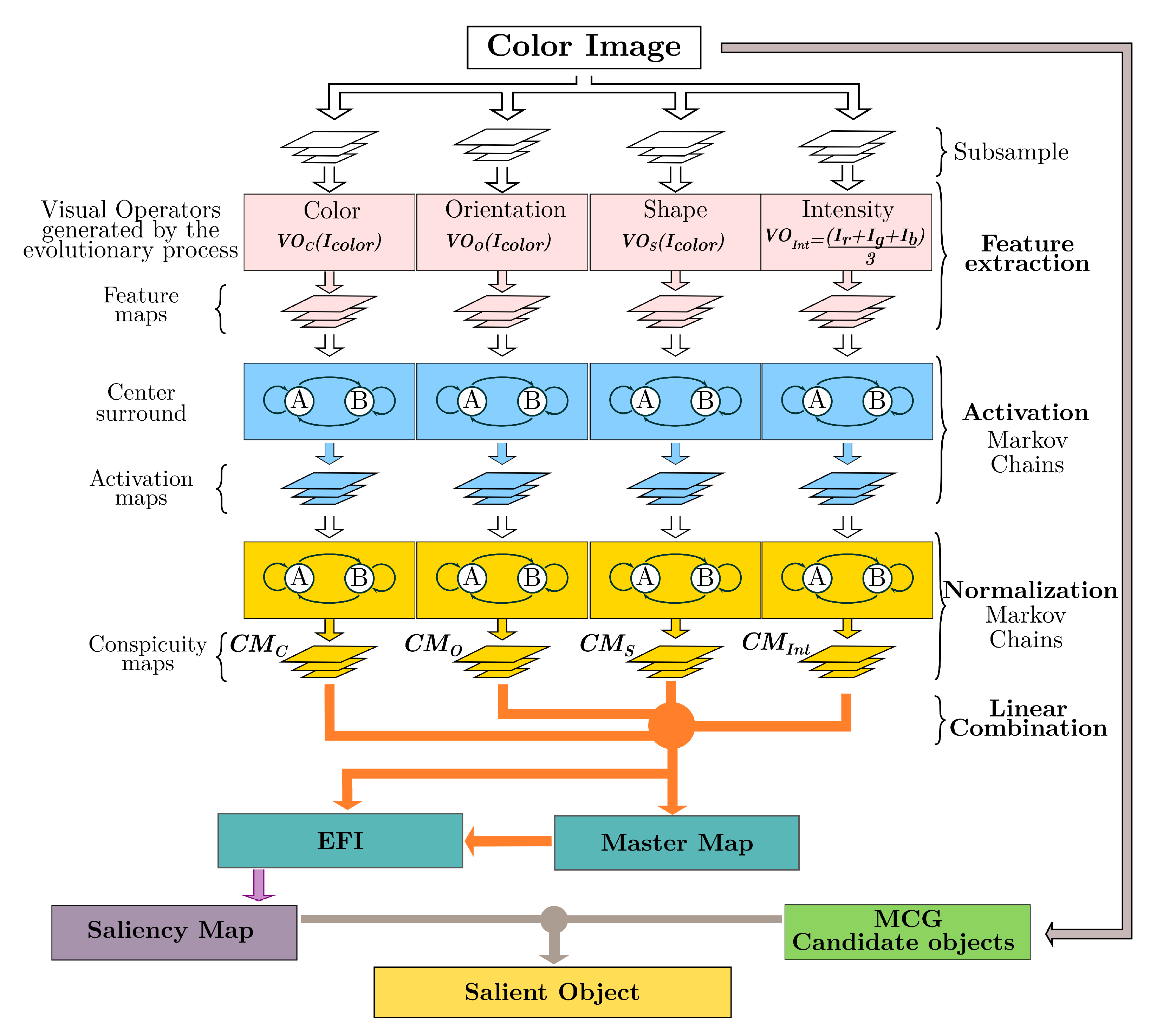
Figure 1 shows the template’s implementation (individual representation) that emulates an artificial dorsal stream (ADS). As we can observe, the whole algorithm represents a complex process based on two models. A neurophysiological model called the two-pathway cortical model—the two-streams hypothesis—and a psychological model called feature integration theory [10]. This last theory states that human beings perform visual attention in two stages. The first is called the preattentive stage, where visual information is processed in parallel over different feature dimensions that compose the scene: color, orientation, shape, intensity. The second stage, called focal attention, integrates the extracted features from the previous stage to highlight the scene’s region (salient object). Hence, the image is decomposed into several dimensions to obtain a set of conspicuity maps, which are then integrated—through a function known as evolved feature integration (EFI)—into a single map called the saliency map. Brain programming (BP) is based on the most popular theory of feature integration for the dorsal stream and the hierarchical representation of multiple layers as in the ventral stream [11]. Note that the template’s design can be adapted according to the visual task. In this work, we focus on designing an artificial dorsal stream. Moreover, BP replaces the data-driven models with a function-driven paradigm. In the function-driven process, a set of visual operators ( V O s ) is fused by synthesis to describe the image’s properties to tackle object location and recognition tasks.
Intelligence data analysis (IDA) is a new research area concerned with analyzing data science effectively to discover meaningful information to improve decisions for real-world problems effectively [12]. Traditionally, deductive reasoning is the method of preference since problems can be naturally explained under pure reasoning, and salient object detection is no exception. However, inductive reasoning, largely represented under the umbrella of deep learning, is the flagship approach of a new wave of methodologies following the design by synthesis [13]. So far, researchers have approached IDA problems with a growing set of bioinspired techniques founded on synthesis with advantages, and disadvantages [14]. Gupta et al. describe a deep learning methodology to improve SOD with heuristic processes following empirical assessment [15]. While a consensus about which process to apply has not been arrived at yet, we believe that a balanced methodology between analysis and synthesis is a way of combining the best of both approaches [16]. Merging both approaches for image complex problems is an active research area. Santamaría et al. provide an overview on the latest nature-inspired and metaheuristic-based image registration algorithms [17]. Iqbal et al. introduce the idea of applying learning classifier systems to SOD research [18]. Brain programming has proved its robustness against adversarial attacks, a hot topic in machine learning, for the problem of image classification [19]. Finally, the honeybee search algorithm is applied to 3D reconstruction and visual tracking by [20,21].
Figure 1. Brain programming implementation of the dorsal stream using the combination of visual saliency and image segmentation algorithms. We propose discovering a set of visual operators ( V O s ) and the evolutionary feature integration (EFI) within the template through artificial evolution. The whole design makes a design balance between the human designer (deductive reasoning) and the computer (symbolic learning).
Applsci 12 10686 g001
This paper is organized as follows. First, we outline the related work briefly to highlight the research direction and contributions of our work. Next, we detail the construction of the ADS template using an adaptation of graph-based visual saliency (GBVS) combined with the multiscale combinatorial grouping (MCG) to an evolutionary machine learning algorithm. Then, we present the results of the evolutionary algorithm to illustrate the benefits of the new proposal. Finally, we finish the article with our conclusions and future work on the automate design of brain models.

2. Related Work

For a learning algorithm design technique to be well received, it needs to solve several analysis levels regarding the automated generation or improvement of algorithms for solving a particular or broad set of problems [22]. A significant critique of deep learning is the opacity generating problems, such as lack of interpretability, reusability, and generality. Scientists depend on complex computational systems that are often ineliminably opaque, to the detriment of our ability to give scientific explanations and detect artifacts. Here, we follow a strategy for increasing transparency based on three levels of explanation about what vision is, how it works, and why we still lack a general model, solution, or explanation for artificial vision [23]. The idea follows a goal-oriented framework where we study learning as an optimization process [16]. The first is theoretical transparency or knowledge of the visual information processing whose design is the computation goal. The second is algorithmic transparency or knowledge of visual processing coding. Finally, the third level is execution transparency, or knowledge of implementing the program considering specific hardware and input data.
Visual attention has a long history, and we recommend the following recent articles to the interested reader to learn more about the subject [24,25,26,27]. However, to put it into practice, it is better to look for information about benchmarks [28,29,30]. In the present work, we select the study of Li et al. since it provides an extensive evaluation of fixation prediction and salient object segmentation algorithms, as well as statistics with standard datasets [30]. They provide a framework focusing on the performance of GBVS against several state-of-the-art proposals. The study also explains how fixation prediction algorithms adapt to salient object detection by incorporating a segmentation stage. Fixation prediction algorithms target predicting where people look in images. Salient object detection focus on a wide range of object-level computer vision applications. Since fixation prediction originated from cognitive and psychological communities, the goal is to understand the biological mechanism. Salient object detection does not necessarily need to understand biological phenomena.
Regarding the second level of explanation (algorithmic transparency) or the knowledge of the visual processing coding, we can observe two different approaches to incorporating learning into such a study. A deep learning technique exemplifies the first (DHSNet—deep hierarchical saliency network [31]) since it is used as a building block in [6]. This method is a fully convolutional network (FCN), a well-known method designed to address the limitations of multi-layer perceptron (MLP)-based methods. FCN architectures lead to end-to-end spatial saliency representation learning and fast saliency prediction within a single feed-forward process. FCN-based methods are now dominant in the field of computer vision. Since DHSNET results rank worst in the proposed benchmark, we decided to train and test two more FCN approaches:
  • BASNet—boundary-aware salient object detection [32];
  • PiCANet–learning pixel-wise contextual attention for saliency [33].
Furthermore, we repeat the experiments to compare our proposal with state-of-the-art methodologies to know the limitations of the proposed method described in this paper.
The second methodology is represented by evolutionary computation, applying genetic programming. We identify two representative works. In [6], the contribution is oriented toward the mechanical design of combination models using genetic programming. The proposed approach automatically selects the algorithms to be combined, and the combination operators use a set of candidate saliency detection methods and a set of combination operators as input. This idea follows a long history in computer vision about combination models. To achieve good results, the authors rely on complex algorithms, such as DHSNet, as building blocks to the detriment of transparency since the method does not enhance the complex algorithms in the function set but only the output.
Since fixation prediction algorithms are complex heuristics, another alternative is to work directly with some essential parts of the algorithm to attempt to improve/discover the whole design. In [5], genetic programming generates visual attention models—fixation prediction algorithms—to tackle salient object segmentation. However, the authors took a step back, returning to the first stage—theoretical transparency—and revisited Koch et al., looking for a suitable model susceptible to optimization [34]. Dozal et al. develop an optimization-based approach introducing symbolic learning within crucial parts of the complete model, using it as a basic algorithm that serves the purpose of a template. This algorithm uses as a foundation the code reported in Itti’s work [35]. In this way, Dozal et al. attempt to fulfill the second stage—algorithmic transparency—since they contemplate the difficulty of articulating the whole design exposed by Treisman and Gelade through heuristic search.
In summary, it is difficult to delegate all practical aspects to the computer according to the genetic programming paradigm. This way of looking for visual attention programs has already impacted practical applications, such as visual tracking [36,37]. This method searches for new alternatives in the feature integration theory (FIT) processes. That includes processes for acquiring visual features, the computation of conspicuity maps, and integrating features. Nevertheless, a drawback is that the visual attention models evolved to detect a particular/single object in the image.
In this work, we would like to identify all foreground regions and separate them from the background. Note that the foreground can contain any object on a particular database. Proper identification of the foreground from the background was the problem approached by Contreras et al. and is known as salient object detection, a hot topic exclusively studied nowadays from a deep learning viewpoint. The idea is to replace Itti’s algorithm with the proposal published in [38] and the further adaptation and benchmark described in [30]. We corroborated the results, testing with more databases [24] and deep learning methodologies [27].
We highlight the following contributions:
1.
The study of salient object detection using a symbolic approach methodology provides a way to extend previous human-made designs with learning capabilities. The algorithms defeat DHSNet and obtain competitive outcomes against recent deep learning models.
2.
Learning is an inductive process, and as with any heuristic/stochastic method, we need methodologies that corroborate the results through statistical approaches. We use k-fold cross-validation to provide evidence about the proposed methodology’s robustness.
3.
In BP, the template refers to a deductive reasoning strategy combined with an inductive learning approach powered by genetic programming. The whole methodology describes an inferential knowledge system that naturally fulfills the requirement of being explainable. The programs evolved by artificial evolution complete the flowchart following logical reasoning.
Koch and coworkers adapt Treisman and Gelade’s theory into essential computational reasoning [34]. Itti’s algorithm accomplishes two stages: (1) visual feature acquisition and (2) feature integration. It consists of visual-feature extraction and computation of visual and conspicuity maps, feature combination, and the saliency map. GBVS is not different from Itti’s implementation. However, it makes a better description of the technique through Markov processes. The idea is to adapt the GBVS algorithm to the symbolic framework of brain programming. Figure 1 depicts the proposed algorithm that discovers multiple functions through artificial evolution. GBVS is a graph-based bottom-up visual salience model. It consists of three steps: first, extraction of features from the image; second, creation of activation maps using the characteristic vectors; and third, normalization of activation maps and combining these maps into a master map. We adapt the algorithm described in [5] with the new proposal using four dimensions: color, orientation, shape, and intensity. In Koch’s original work, there are three dimensions, each approached with a heuristic method, and the same for the integration step. We apply the set of functions and terminals provided in [39] with a few variants to discover optimal heuristic models for each stage. This algorithm uses Markov chains to generate the activation maps. Researchers consider this approach “organic” because, biologically, individual “nodes” (neurons) exist in a connected, retinotopically organized network (the visual cortex) and communicate with each other (synaptic activation) in a way that results in emergent behavior, including quick decisions about which areas of a scene require additional processing.

3. Methodology

BP aims to emulate the behavior of the brain through an evolutionary paradigm using neuroscience knowledge for different vision problems. The first studies to introduce this technique [5,8] focused on automating the design of visual attention (VA) models and studied the way it surpasses previous human-made systems developed by VA experts. To perceive salient visual features, the natural dorsal stream in the brain has developed VA as a skill through selectivity and goal-driven behavior. The artificial dorsal stream (ADS) emulates this practice by automating acquisition and integration steps. Handy applications for this model are tracking objects from a video captured with a moving camera, as shown in [36,37].
BP is a long process consisting of several stages summarized in two central ideas correlated with each other. First, the primary goal of BP is to discover functions capable of optimizing complex models by adjusting the operations within them. Second, a hierarchical structure inspired by the human visual cortex uses function composition to extract features from images. It is possible to adapt this model depending on the task at hand, e.g., the focus of attention can be applied to saliency problems [5], or the complete artificial visual cortex (AVC) can be used for categorization/classification problems [8]. This study uses the ADS, explained to a full extent in the following subsections, to obtain as a final result the design of optimal salient object detection programs which satisfy the visual attention task. Appendix A provides pseudo codes of all relevant algorithms for the interested reader.

3.1. Initialization

BP begins with a randomized generation along an evolutionary process defined by a set of initialization variables such as population size, size of solutions or individuals, or crossover-mutation probabilities. An individual represents a computer program written with a group of syntactic trees embedded into hierarchical structures. In this work, individuals within the population contain functions corresponding to one of the four available visual operators ( V O ). Table 1 shows the functions and terminals used for each V O or visual map ( V M ). The table includes arithmetic functions between two images A and B, transcendental and square functions, square root function, image complement, color opponencies (red–green and blue–yellow), dynamic threshold function, arithmetic functions between an image A, and a constant k. It also includes transcendental operations with a constant k and the spherical coordinates of the DKL color space. The table also incorporates round, half, floor, and ceil functions over an image A, dilation and erosion operators with the disk, square, and diamond structure element ( S E ), skeleton operator over the image A, finding the perimeter of objects in the image A, hit-or-miss transformation with the disk, square, and diamond structures. Additionally, we include morphological top-hat and bottom-hat filtering over the image A, opening and closing morphological operator on A, absolute value applied to A, and the addition and subtraction operators. Finally, we add infimum and supremum functions between images A and B, the convolution of the image A, a Gaussian filter with σ = 1 or 2, and the derivative of the image A along direction x and y. Note that all dimensions include elementary functions since these can be employed to compose high-level properties (invariance to rotation, translation, scaling, and illumination) through the template design.
Table 1. Functions and terminals for the ADS.
Functions for E V O O Terminals for E V O O
A + B , A B , A × B , A / B , | A | , | A + B | , | A B | , log 2 ( A ) , A / 2 , A 2 , A , k × A , A / k , A 1 / k , A k , ( 1 / k ) + A , A ( 1 / k ) , G σ = 1 ( A ) , G σ = 2 ( A ) , D x ( A ) , D y ( A ) , r o u n d ( A ) , A , A , i n f ( A , B ) , s u p ( A , B ) , t h r ( A ) , A t t e n u a t e B o r d e r s ( A ) , C o n v G a b o r ( A ) I r , I g , I b , I c , I m , I y , I k , I h , I s , I v , D x ( I c o l o r ) , D x x ( I c o l o r ) , D y ( I c o l o r ) , D y y ( I c o l o r ) , D x y ( I c o l o r ) , A t t e n u a t e B o r d e r s ( I c o l o r ) , C o n v G a b o r ( I c o l o r ) ,
Functions for E V O C Terminals for E V O C
A + B , A B , A × B , A / B , log 2 ( A ) , e x p ( A ) , | A | , A 2 , A , ( A ) c , t h r ( A ) , r o u n d ( A ) , A , A , k × A , A / k , A 1 / k , A k , ( 1 / k ) + A , A ( 1 / k ) I r , I g , I b , I c , I m , I y , I k , I h , I s , I v , D K L r , D K L Φ , D K L Θ , O p r g ( I ) , O p b y ( I )
Functions for EVOSTerminals for EVOS
A + B , A B , A × B , A / B , | A | , k × A , A / k , A 1 / k , A k , ( 1 / k ) + A , A ( 1 / k ) , r o u n d ( A ) , A , A , A S E d , A S E s , A S E d m , A S E d , A S E s , A S E d m , S k ( A ) , P e r i m ( A ) , A S E d , A S E s , A S E d m , T h a t ( A ) , B h a t ( A ) , A S E s , A S E s , t h r ( A ) I r , I g , I b , I c , I m , I y , I k , I h , I s , I v
Functions for E F I Terminals for E F I
A + B , A B , A × B , A / B , | A | , | A + B | , | A B | , k × A , A / k , A 1 / k , A k , ( 1 / k ) + A , A ( 1 / k ) , H i s t ( A ) , r o u n d ( A ) , A , A , t h r ( A ) , ( A ) 2 , A , e x p ( A ) , G σ = 1 ( A ) , G σ = 2 ( A ) , D x ( A ) , D y ( A ) C M d , D x ( C M d ) , D x x ( C M d ) , D y ( C M d ) , D y y ( C M d ) , D x y ( C M d )

3.2. Individual Representation

We represent individuals using a set of functions for each V O defined in Section 3.3. Entities are encoded into a multi-tree architecture and optimized through evolutionary crossover and mutation operations.
The architecture uses three syntactic trees for each evolutionary visual operator ( E V O O , E V O C , E V O S ) regarding orientation, color, and shape. We then merge the C M s produced by the center-surround process–including feature and activation maps–using an EFI tree, generating a saliency map (SM); therefore, we apply four syntactic trees. Section 3.3.1 provides details about the usage of these E V O s ; additionally, Figure 1 provides a graphical representation of the complete BP workflow. After initializing the first generation of individuals, the fitness of each solution is tested and used to create a new population.

3.3. Artificial Dorsal Stream

The ADS models some components of the human visual cortex, where each layer represents a function achieved by synthesis through a set of mathematical operations; this constitutes a virtual bundle. We select visual features from the image to build an abstract representation of the object of interest. Therefore, the system looks for salient points (at different dimensions) in the image to construct a saliency map used in the detection process. The ADS comprises two main stages: the first acquires and transforms features in parallel that highlight the object, while in the second stage, all integrated features serve the goal of object detection.

3.3.1. Acquisition and Transformation of Features

In this stage, different parts of the artificial brain automatically separate basic features into dimensions. The entrance to the ADS is a color image I defined as the graph of a function.
Definition 1
(Image as the graph of a function). Let f be a function f : U R 2 R . The graph or image I of f is the subset of R 3 that consists of the points ( x , y , f ( x , y ) ) , in which the ordered pair ( x , y ) is a point in U and f ( x , y ) is the value at that point. Symbolically, the image I = { ( x , y , f ( x , y ) ) R 3 | ( x , y ) U } .
From this definition, we can highlight how images are variations in light intensity along the two-dimensional plane of camera sensors. Regarding visual processing for feature extraction of the input image, we consider multiple color channels to build the set I c o l o r = { I r , I g , I b , I c , I m , I y , I k , I h , I s , I v } , where each element corresponds to the color components of the RGB (red, green, blue), HSV (hue, saturation and value) and CMYK (cyan, magenta, yellow and black) color spaces. We define the optimization process by formulating an appropriate search space and evaluating functions.

3.3.2. Feature Dimensions

In this step, we obtain relevant characteristics from the image by decomposing it and analyzing key features. Three E V O s transform the input picture I c o l o r through each V O defined as E V O d : I c o l o r V M d and applied in parallel to emphasize specific characteristics of the object. Note that the fourth V M I n t is not evolved and is calculated with the average of the RGB color bands. These E V O s are operators generated in Section 3.2. Individuals–programs represent possible configurations for feature extraction that describe input images and are optimized using the evolutionary process. We perform these transformations to recreate the process of extracting information following the FIT. When applying each operator, a V M generated for each dimension represents a partial procedure within the overall process. Each V M is a topographic map that represents, in some way, an elementary characteristic of the image.

3.4. Creating the Activation Maps

After selecting the visual operators generated by the evolutionary process, the feature maps complete the feature extraction. Next, the algorithm creates activation maps as follows. Suppose we are given a feature map M : [ n ] 2 R the goal is to compute an activation map for each dimension A : [ n ] 2 R such that locations ( i , j ) [ n ] 2 on the image, or as a proxy, M ( i , j ) , that are somehow unusual in its neighborhood will correspond to high values of activation A. The dissimilarity of M ( i , j ) and M ( p , q ) is given by
d ( ( i , j ) | | ( p , q ) ) log M ( i , j ) M ( p , q ) .

3.5. A Markovian Approach

Consider a fully connected graph denoted as G A . For each node M with its indexes, ( i , j ) [ n ] 2 is connected to the other nodes. The edge point of a node in the two-dimensional plane ( i , j ) to the node ( p , q ) will be the weight and is defined as follows:
w 1 ( ( i , j ) , ( p , q ) ) d ( ( i , j ) | | ( p , q ) ) · F ( i p , j q ) ,
where
F ( a , b ) e x p ( a 2 + b 2 ) 2 σ 2 ,
Moreover, σ is a free parameter of the algorithm. Thus, the weight of the edge from node ( i , j ) to node ( p , q ) is proportional to their dissimilarity and their closeness in the domain of M. It is possible then to define a Markov chain on G A by normalizing the weights of the outbound edges of each node to 1, and drawing an equivalence between node states, and edges’ weight-transition probabilities.

3.6. Normalizing an Activation Map

This step is crucial to any saliency algorithm and remains a rich study area. GBVS proposes another Markovian algorithm, and the goal of this step is a mass concentration in the activation maps. The authors construct a graph G N with n 2 nodes labeled with indices from [ n ] 2 . For each node ( i , j ) and ( p , q ) connected, they introduce an edge from
w 2 ( ( i , j ) , ( p , q ) ) A ( p , q ) · F ( i p , j q ) .
Once again, the algorithm normalizes each node’s output edges, treating the resulting graph as a Markov chain, making it possible to calculate the equilibrium distribution over the nodes. The mass will flow preferentially to those nodes with high activation. The artificial evolutionary process works with the modified version of GBVS. We can add the MCG during the evolution or after to improve the results since the image segmentation computational cost with this algorithm is very high.

3.7. Genetic Operations

We follow the approach detailed in [5], where the template represents an individual containing a set of V M s coded into an array of trees similar to a chromosome and where each visual operator within the chromosome is a gene code. In other words, the chromosome is a list of visual operators ( V O s ), and each V O is a gene. Therefore, we apply four genetic operators:
  • Chromosome-level crossover. The algorithm randomly selects a crossing point from the list of trees. The process builds a new offspring by unioning the first parent’s left section with the second parent’s right section.
  • Gene level crossover: This operator selects two V O s , chosen randomly, from a list of trees, and for each function of both trees (genes), the system chooses a crossing point randomly, then the sub-trees under the crossing point are exchanged to generate two new visual operators. Therefore, this operation creates two new children chromosomes.
  • Chromosome-level mutation: The algorithm randomly selects a mutation point within a parent’s chromosome and replaces the chosen operator completely with a randomly generated operator.
  • Gene-level mutation: Within a visual operator, randomly chosen, the algorithm selects a node, and the mutation operation randomly alters the sub-tree that results below this point.
Once we generate the new population, the evolutionary process continues, and we proceed to evaluate the new offspring.

3.8. Evaluation Measures

Evolutionary algorithms usually apply a previously defined fitness function to evaluate the individuals’ performance. BP designs algorithms using the generated E V O s to extract features from input images through the ADS hierarchical structure depicted in Figure 1. Experts agree on evaluating the various proposals for solutions to the problem of salient object detection. In this work, we follow the protocol detailed with source code in [29] and apply two main evaluation measures: precision–recall and F-measure. Researchers represent the first through Equation (5):
P r e c i s i o n = | B M G | | B M | , R e c a l l = | B M G | | G | .
To compute a saliency map S, we convert it to a binary mask B M , and compute P r e c i s i o n and R e c a l l by comparing B M with ground-truth G. In this definition, binarization is a critical step in the evaluation. The benchmark offers a method based on thresholds to generate a precision–recall curve. The second measure (Equation (6)) is made with this information to obtain a figure of merit:
F β = ( 1 + β 2 ) P r e c i s i o n × R e c a l l β 2 P r e c i s i o n + R e c a l l .
This expression comprehensively evaluates the quality of a saliency map. The F-measure is the weighted harmonic mean of precision and recall. In the benchmark, β 2 is set to 0.3 to increase the importance of the precision value.
We calculate both evaluations with two variants. In our first approach, we obtain the maximum F-measure considering different thresholds for each image during the binarization process. Then, we calculate the average of all photos in the training or testing set; see [5]. The benchmark uses the second variant, which consists of calculating the average that results from varying the thresholds and then reporting the maximum resulting from evaluating all the images. We will use both approaches during the experiments to ensure that such evaluations do not change the rankings.

4. Experiments and Results

Designing machine learning systems requires the definition of three different components: algorithm, data, and measure. This section evaluates the proposed evolutionary algorithm with a standard test. Thus, the goal is to benchmark our algorithm against external criteria. This way, we need to run a series of tests based on data and measures from well-known experts. Finally, we contrast our results with several algorithms in the state-of-the-art.
This research follows the protocol detailed in [30]. This benchmark is of great help because it allows us to access the source code of various algorithms to make a more exhaustive comparison. This benchmark also analyzes blunt flaws in the design of salience benchmarks known as database design bias produced by emphasizing stereotypical salience concepts. This benchmark extensively evaluates fixation prediction and salient object segmentation algorithms. We focus on the salient object detection part, consisting of three databases FT, IMGSAL, and PASCAL-S. We present complete results next. Additionally, we include a test of the best program with the databases proposed in [6].

4.1. Image Databases

FT is a database with 800 images for training and 200 for testing. Authors of the benchmark reserve this last set of 200 images for comparison. We use the training dataset to perform a k-fold technique ( k = 5 ) to find the best individual. We randomly partitioned the training dataset into five subsets of 160 images. Each execution was run considering the parameters from Table 2. We retained a single subset of the k subsets as the validation data for testing the model and used the remaining k 1 subsets as training data. Table 3 reports the best program results for 30 executions in the k-fold technique. We follow the same procedure in the PASCAL-S database [40], and the final results are given in Figure 3 while adding ocular fixation information and object segmentation labeling. The training set consists of 680 images, while the test set consists of 170 images for comparison. We divide the training set into five subsets of 136 images to perform a 5-fold cross validation to discover the best algorithm. Finally, we run the experiments on the IMGSAL dataset containing 235 images. The database splits into 188 images for training and 47 images for testing. We select 185 from the training set and split it into five subsets of 37 images to perform a 5-fold cross validation.
Table 2. Main parameters settings of the BP algorithm.
ParametersDescription
Generations30
Population size30
InitializationRamped half-and-half
Crossover at chromosome level0.8
Crossover at gene level0.8
Mutation at chromosome level0.2
Mutation at gene level0.2
Tree depthDynamic depth selection
Dynamic maximum depth7 levels
Maximum actual depth9 levels
SelectionTournament selection
with lexicographic
parsimony pressure.
ElitismKeep the best individual
FT contains a diverse representation of animate and inanimate objects with image sizes ranging from 324 × 216 to 400 × 300 . PASCAL-S contains scenes of domestic animals, persons, and means of air and sea transport with image sizes ranging from 200 × 300 up to 375 × 500 . Finally, IMGSAL has wild animals, flora, and different objects and persons with image sizes of 480 × 640 . All images in the three datasets came with their corresponding ground truth. The manual segmentation was carefully made in FT and PASCAL-S datasets to obtain accurate ground truth. At the same time, IMGSAL provides a ground truth that was purposefully segmented following a rough segmentation to illustrate a real-world case where humans imprecisely indicate an object’s location.

4.2. Experiments with Dozal’s Fitness Function on GBVSBP

Table 3 details the experimental results after applying the k-fold cross-validation method on the FT database. As we can observe, BP optimizes the model scoring the highest value of 78.18 % for the best program during training at the first run and the third fold, while achieving 77.67 % during testing in the fourth run but at the fourth fold. σ remains low during the experimental runs. BP scores its highest value σ = 2.54 in the fourth testing run while achieving σ = 0.45 and σ = 1.51 during the sixth run for training and testing, respectively. The methodology average scores its highest fitness of 76.72 % for training and 75.17 % for testing. Table 4 presents the best solution. The selected program corresponds to the training stage for this kind of table.
Table 3. Performance of the best individuals of the GBVSBP model for all FT database runs. Each pair of training and testing corresponds to one experiment of the k-fold. Therefore, we obtain 30 executions of our system and report the standard deviation for each run set.
FT
FoldRun 1Run 2Run 3Run 4Run 5Run 6
TrngTestTrngTestTrngTestTrngTestTrngTestTrngTest
175.3476.1075.0773.9777.5776.7576.9875.2977.3475.7477.0875.36
274.8871.6072.9269.8175.1072.9774.6571.2773.6271.8776.4172.25
378.1876.5876.6971.7777.0372.9776.7572.1876.6872.3977.0172.21
475.3077.0574.7874.2574.9071.4775.8677.6774.6076.1377.0374.98
575.1574.5473.1473.4574.7474.9774.6274.1775.1875.0676.0974.37
Average75.7775.1774.5272.3275.8773.8375.7774.1275.4874.2476.7273.83
σ 1.362.211.541.971.332.051.122.541.521.970.451.51
Table 4. Program structure of the operators corresponding to the best solution for the FT database. We select this solution from the 30 executions of Table 3. The final solution is simple, basically using color-chosen bands.
      EVO d and EFI OperatorsFitness
     E V O O = I k Training = 0.7818
     E V O C = I b + 1.00 Testing = 0.7658
      E V O S = t o p h a t ( I m × 0.31 )
     E F I = ( C M C ) 2 2
Table 5 details the experimental results after applying the k-fold cross-validation method on the IMGSAL database. The fitness function results on this dataset show high variability since, in training, the results range from 72.49 % in the fourth run to 57.37 % in the second run. The high dispersion is due to the complexity of the problem generated by poor manual segmentation. The experiment shows an average oscillating between 62.60 % and 68.52 % for training with σ = 3.72 and σ = 1.52 , respectively. On the other hand, during testing, the algorithm’s highest score on average is 67.04 % with σ = 2.48 . Table 6 reports the best solution.
The experimental results of the GBVSBP model with the PASCAL-S database show excellent stability, as seen in Table 7 with a low standard deviation, especially in training with the first run, scoring 1.58. During training, fitness reaches its highest in the fifth fold of run 6, scoring 66.39 % , while on average, the fifth run scores first place with 63.45 % . Regarding the testing stage, the algorithm scores the best individual at the third fold with 67.66 % , and on average, the best run is the fifth with 63.63 % . Table 8 presents the best set of trees.
Table 5. Performance of the best individuals of the GBVSBP model for all IMGSAL database runs. Each pair of training and testing corresponds to one experiment of the k-fold. Therefore, we obtain 30 executions of our system and report the standard deviation for each run set.
IMGSAL
FoldRun 1Run 2Run 3Run 4Run 5Run 6
TrngTestTrngTestTrngTestTrngTestTrngTestTrngTest
168.3066.8867.6265.2968.8664.2872.4968.6666.2365.4559.2462.2
265.2364.0667.1064.7666.7964.8264.1870.1269.2569.6966.2664.96
368.8666.2564.9962.7360.8461.8264.3965.2668.2263.9366.762.42
462.7270.9157.3761.2768.4267.1666.5266.8768.5267.1761.8764.56
570.7467.1068.9965.4366.2660.3762.8662.7370.3666.658.9461.45
Average67.1767.0465.2163.9066.2363.6966.0966.7368.5266.5762.6063.12
σ 3.182.484.611.823.202.653.812.891.522.143.721.55
Table 6. Program structure of the operators corresponding to the best solution for the IMGSAL database. We select this solution from the 30 executions of Table 5. The final solution applies filters to selected color images and derivatives to the conspicuity maps.
     EVO d and EFI OperatorsFitness
    E V O O = ( ( G ( σ = 1 ) ( G ( σ = 1 ) ( I v ) ) 0.44 ) 0.69 ) Training = 0.7249
    E V O C = ( I c 0.44 ) Testing = 0.6866
    E V O S = I m
    E F I = G ( σ = 2 ) ( D y ( D y ( C M C ) ) )
Table 7. Performance of the best individuals of the GBVSBP model for all PASCAL-S database runs. Each pair of training and testing corresponds to one experiment of the k-fold. Therefore, we obtain 30 executions of our system and report the standard deviation for each run set.
PASCAL-S
FoldRun 1Run 2Run 3Run 4Run 5Run 6
TrngTestTrngTestTrngTestTrngTestTrngTestTrngTest
163.5862.3162.9261.8365.1965.3362.2761.3462.8463.1263.7962.25
261.5358.9264.7057.5163.0256.8864.6459.8065.2958.8164.5058.57
361.5864.6163.4765.4662.1864.1363.7165.2263.2067.6659.7164.90
459.6062.8258.2059.7759.2360.8760.4563.6859.7261.7859.8460.63
563.2065.8164.4663.2563.9063.4766.0364.5566.2266.7966.3966.78
Average61.9062.8962.7561.5662.7062.1463.4262.9263.4563.6362.8562.83
σ 1.582.632.643.072.243.362.152.282.523.642.962.99
Table 8. Program structure of the operators corresponding to the best solution for the PASCAL-S database. We select this solution from the 30 executions of Table 7. The final solution consists of a combination of different structures. The first visual operator uses a filter and derivative over I s . The second operator uses algebraic operations (addition and subtraction between color bands). The shape dimension uses I m , and the feature integration applies derivatives to the conspicuity map of color.
   EVO d and EFI OperatorsFitness
   E V O O = ( G ( σ = 1 ) ( D y ( I s ) ) ) Training = 0.6639
   E V O C = ( ( ( ( ( I m 0.62 ) 0.62 ) + I y ) + ( I y + I v ) ) + ( I y + I v ) ) Testing = 0.6678
   E V O S = I m
   E F I = D y ( D y ( C M C ) )
The experiment with our second model GBVSBP+MCG and the FT database shows outstanding results compared to the previous model, see Table 9. Another remarkable difference is the stability during training regarding the standard deviation, whose performance decreases while testing the best models, where four values score above σ = 3 . Meanwhile, in the testing stage, the best individual achieves 95.06 % in the second run. On average, the algorithm discovers the best individuals considering all folds in the first run with 93.47 % , while the second run reports the best results with an average of 92.13 % . Table 10 shows the best solution.

4.3. Experiments with Benchmark’s Score

In the second round of experiments, we adapt the algorithm to use the proposed benchmark’s score as a fitness function, as explained earlier; see Section 3.8. From now on, all report experiments consider this way of evaluation. Table 11 provides the results of the k-fold experimentation considering the GBVSBP algorithm with the FT database, while Table 12 provides the corresponding best individual. As can be seen, there is a decrease, but the ranking remains unaltered, as we verified with the solutions. The results considering the dataset IMGSAL are in Table 13 and Table 14, while those of PASCAL-S are in Table 15 and Table 16 respectively, while Table 17 provides partial results with the GBVSBP+MCG model to illustrate the performance.
With this new F-measure, the results obtained show greater stability globally according to Table 11 despite runs 1 and 4 reporting σ = 4.47 and σ = 4.23 . All other values are below 2 % . Despite the decrease, the fitness of the individuals remains competitive as the best individual in the training stage achieves 72.59 % , and the best in the test stage reaches 73.81 % . In this experiment, the last run reflects the highest average fitness considering all folds and for both stages with values of 70.29 % and 69.06 % . Table 12 gives the best set of visual operators.
Table 12. Program structure of the operators corresponding to the best solution for the FT database. We select this solution from the 30 executions of Table 11. This final solution is simple: a single color channel and algebraic operations between color channels for the first two visual operators. The third uses a threshold, and the last one applies derivatives.
   EVO d and EFI OperatorsFitness
   E V O O = I r Training = 0.7259
   E V O C = ( ( ( I k + I m ) + I m ) + I m ) Testing = 0.7365
   E V O S = t h r e s h o l d ( I y )
   E F I = D x ( D y ( C M S ) )
Table 13. Performance of the best individuals of the GBVSBP model for all IMGSAL database runs. Each pair of training and testing corresponds to one experiment of the k-fold. Therefore, we obtain 30 executions of our system and report the standard deviation for each run set.
IMGSAL
FoldRun 1Run 2Run 3Run 4Run 5Run 6
TrngTestTrngTestTrngTestTrngTestTrngTestTrngTest
157.1960.1660.0960.1765.3563.4562.0560.3165.0962.2060.2460.8
256.1259.9455.5560.2563.4763.3463.9463.4460.4160.5159.8460.55
357.5655.9057.9657.9663.7861.9363.5459.4957.4556.3456.9760.30
457.4459.8357.3758.0964.2162.9460.0362.2361.6056.6959.8762.26
559.4958.5757.4159.3062.0160.5462.8662.1358.2857.4862.0857.26
Average57.5658.8857.6859.1563.7662.4462.4861.5260.5658.6459.860.23
σ 1.221.781.631.101.211.221.551.593.022.581.831.83
Fitness results with the GBVSBP model and IMGSAL database show similar behavior as we appreciate in outcomes. For example, the highest average was 63.76 % in the training stage with a σ = 1.21 , while reaching a lowest average of 58.64 % with a σ = 2.58 in the testing stage. As we can appreciate, the results were not as high as the other two datasets since IMGSAL presents difficulties primarily due to poor segmentation when creating the ground truth. Additionally, the results took a long time to be completed (several months) due to the bigger image size. The algorithm reached the best solution on the third run, scoring 65.35 % in training and 63.45 % at testing. Table 14 provides the best solution.
Table 14. Program structure of the operators corresponding to the best solution for the IMGSAL database. We select this solution from the 30 executions of Table 13. This final solution is also simple, using a filter and square root for the first two operators, I m for the third, and the absolute value of filters and derivatives over the conspicuity map of shape.
    EVO d and EFI OperatorsFitness
    E V O O = G ( σ = 1 ) ( I v ) Training = 0.6535
    E V O C = ( I m ) Testing = 0.6345
    E V O S = I m
    E F I = | G ( σ = 1 ) ( D y ( C M S ) ) |
Table 15. Performance of the best individuals of the GBVSBP model for all PASCAL-S database runs. Each pair of training and testing corresponds to one experiment of the k-fold. Therefore, we obtain 30 executions of our system and report the standard deviation for each run set.
PASCAL-S
FoldRun 1Run 2Run 3Run 4Run 5Run 6
TrngTestTrngTestTrngTestTrngTestTrngTestTrngTest
162.0359.7561.3957.5361.8857.9860.7656.0661.6258.7560.8958.19
261.5355.1261.9554.9961.1156.5261.3352.6161.2353.6461.0156.70
359.2858.8360.0861.0859.8460.3260.6059.5759.8261.3359.7161.78
459.5758.3658.2054.2858.5955.9158.6158.9058.2157.1357.8956.44
563.2061.4061.9461.9463.0859.1263.3859.0162.9359.0062.8761.34
Average61.1258.6960.7157.9660.9057.9760.9457.2360.7657.9760.4758.87
σ 1.672.311.603.471.751.821.712.921.812.851.832.54
The experimental results with GBVSBP for the PASCAL-S database have higher similarity because the F-measure has greater stability than previous results. The results show a stable standard deviation between 1.60 and 3.47 for training and testing. We obtain similar behavior in the average results between 60.47 % and 61.12 % for the training stage. The best solution was reached in the fifth fold at the fourth run, scoring 63.38 % during training, while in testing, the algorithm scored 61.94 % . Table 16 shows the best trees.
Table 16. Program structure of the operators corresponding to the best solution for the PASCAL-S database. We select this solution from the 30 executions of Table 15. The final solution is similar to all others discovered by the system. This shows that the proposed programs are independent of the selected dataset.
   EVO d and EFI OperatorsFitness
   E V O O = G ( σ = 1 ) ( G ( σ = 1 ) ( I v ) ) Training = 0.6194
   E V O C = I m Testing = 0.6194
   E V O S = ( d i l a t i o n d i s k ( d i l a t i o n s q u a r e ( e r o s i o n d i s k ( I b ) ) ) )
   E F I = | G ( σ = 2 ) ( D y ( C M M M ) ) |
Table 17. Performance of the best individuals of the GBVSBP + MCG model for all FT database runs. Each pair of training and testing corresponds to one of seven experiments. Then, we report the average, standard deviation, minimum, maximum, and mean for the seven experiments.
FT
FoldRun 1Run 2Run 3Run 4Run 5Run 6
TrngTestTrngTestTrngTestTrngTestTrngTestTrngTest
188.4188.5188.0786.0087.9280.8388.3285.7587.5289.0287.0486.69
Run 1Average σ MinimumMaximumMean
TrngTestTrngTestTrngTestTrngTestTrngTestTrngTest
289.0288.5688.2486.530.563.7587.0480.8389.0289.0288.0786.69
The experimental results with GBVSBP + MCG for the FT database show some loss of aptitude against its counterpart in the first block of experiments ( 5 % in training and 3 % in tests). However, the performance values are more stable with σ = 0.56 for training and σ = 3.75 for testing. In addition to stability, we must bear in mind that the results of this experiment will be much more consistent when the best individual is tested in the benchmark since we are using the same F-measure. As a result, the best results were 89.02 % in training corresponding to the second fold of the first run and 89.02 % at testing discovered in the first fold of the fifth run. Table 18 gives the best set of trees.

4.4. Analysis of the Best Evolutionary Run

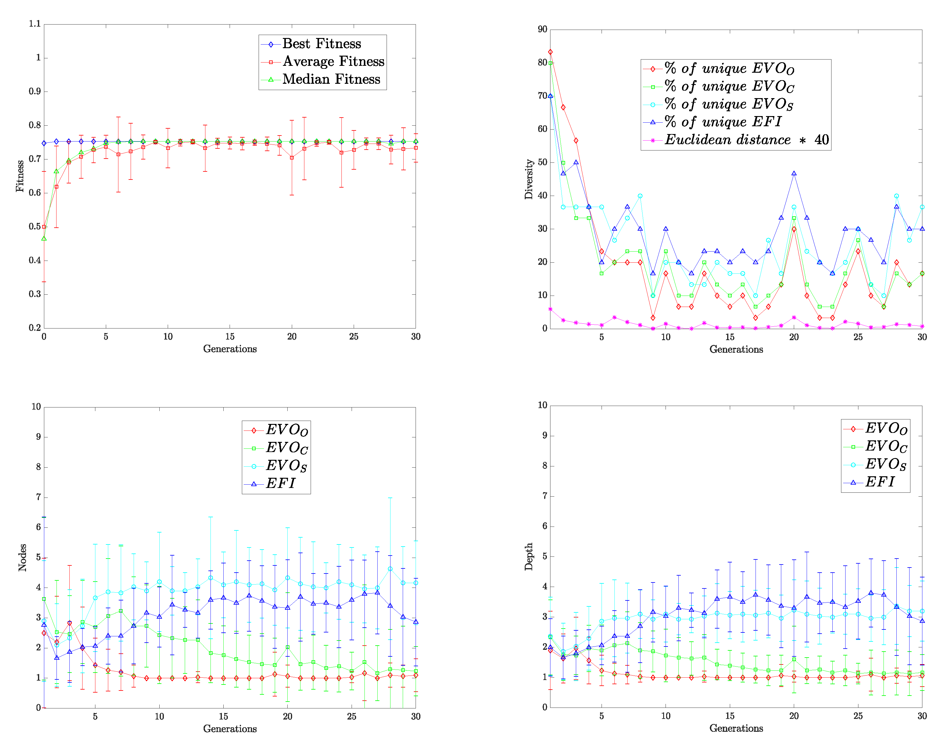
Typical experimental results that illustrate the inner workings of genetic programming are those related to fitness, diversity, number of nodes, and depth of the tree. Figure 2 provides charts giving best fitness, average fitness, and median fitness. The purpose is to detail the performance and complexity of solutions through the whole evolutionary run. As we can observe, artificial evolution scores a high fitness within the first generations. On average, BP converges around the seventh generation. The diversity chart shows solutions’ convergence in all four trees characterizing the program. Compared to the fitness plot, these data demonstrate that despite the differences in diversity during the experiment, the model’s performance remained constant. One of the biggest problems using genetic programming is incrementing a program’s size without a rise in the program’s performance, mainly when the final result cannot be generalized for new data. This problem is called bloat and is usually associated with tree representation. As observed in the last two graphs, the complexity is kept low with the number of nodes below seven and depth below five regarding all trees. These numbers were consistently below the proposed setup for all experiments. The hierarchical structure improves performance and the management of the algorithm’s complexity.

4.5. Comparison with Other Approaches

The values presented above correspond to fitness after the evolutionary cycle of BP to validate our work. The benchmark offers two modalities: one which uses only 60 % of the database and another containing all images; we keep the first option. Table 19 shows the final results achieved on the testing set over ten random splits with our best program considering the FT dataset. Here, we appreciate the final results considering the following algorithms for salient object detection: FT—frequency-tuned, GC—global contrast, SF—saliency filters, PCAS—principal component analysis, and DHSNet. Additionally, we include the original proposal of the artificial dorsal stream named focus of attention (FOA) reported in [5]. Note that we overpass all other algorithms in the benchmark. FT is the most straightforward dataset since all objects are in focus and cover a significant portion of the image. We remark on the poor performance of DHSNet, which contrasts with the results reported in [31]. This poor performance may be because validation images are not part of the training.
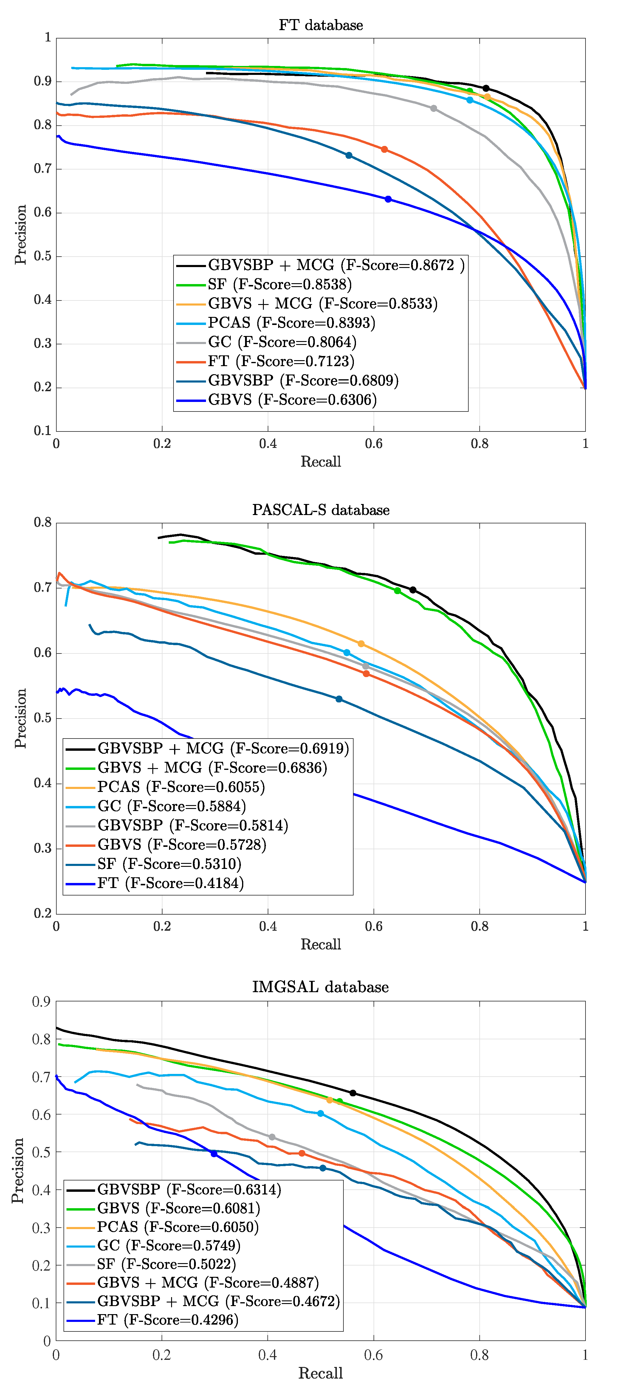
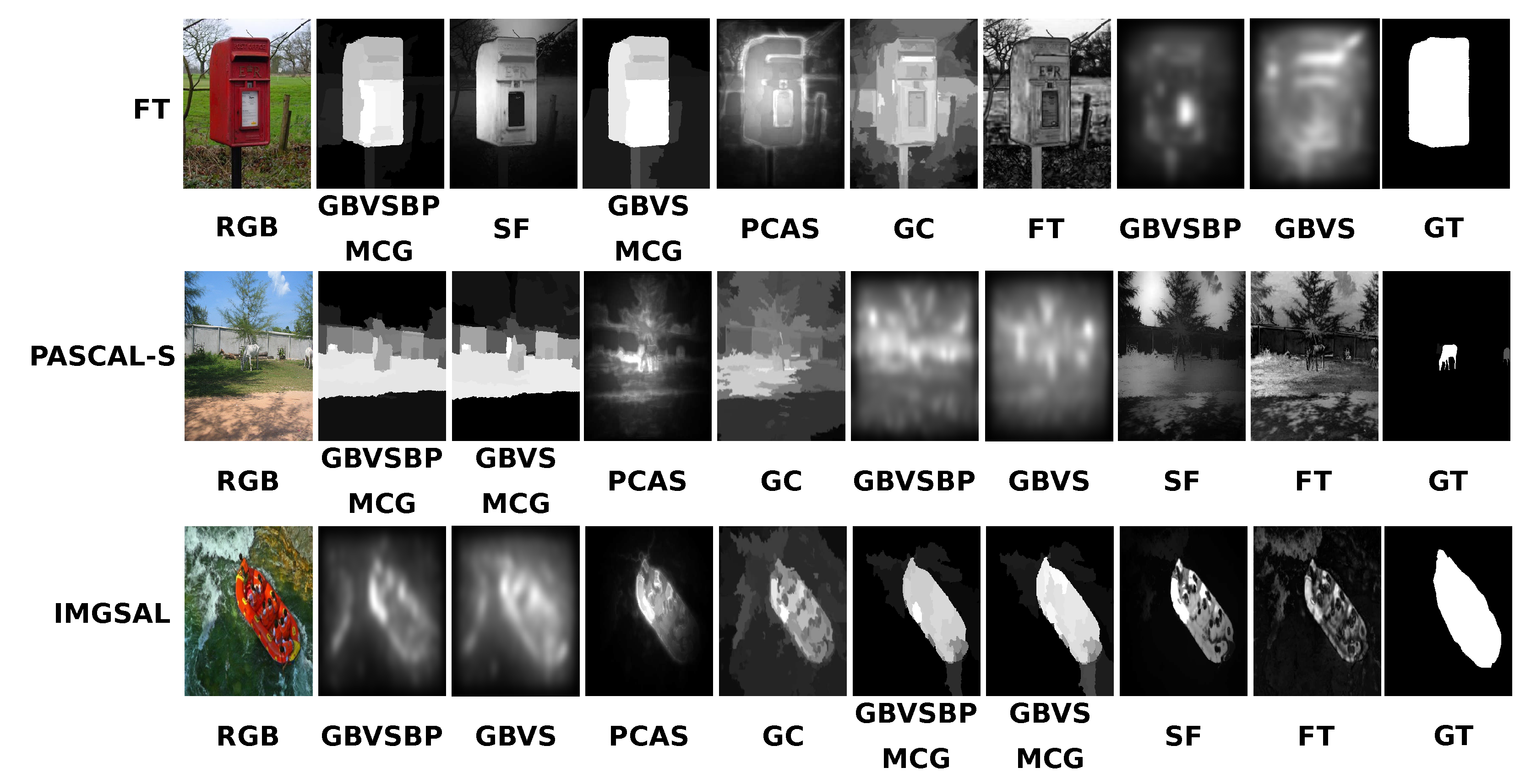
Figure 3 provides precision–recall curves for the benchmark FT, IMGSAL, and PASCAL-S databases. Again, our methods score highest in all datasets. However, GVBSBP + MCG scores highest in the FT and PASCAL-S datasets, while GBVSBP achieves better results in IMGSAL. The rough segmentation in this last dataset worsens the segmentation process. Figure 4 presents image results of all algorithms in the three databases for visual comparison. According to the results of Figure 3 our methods achieve outstanding results; however, we provide the following images to spot some challenges in the benchmark. The rows provide the best method (leftmost) and worst method (rightmost), starting with the original and finalizing with the ground truth.
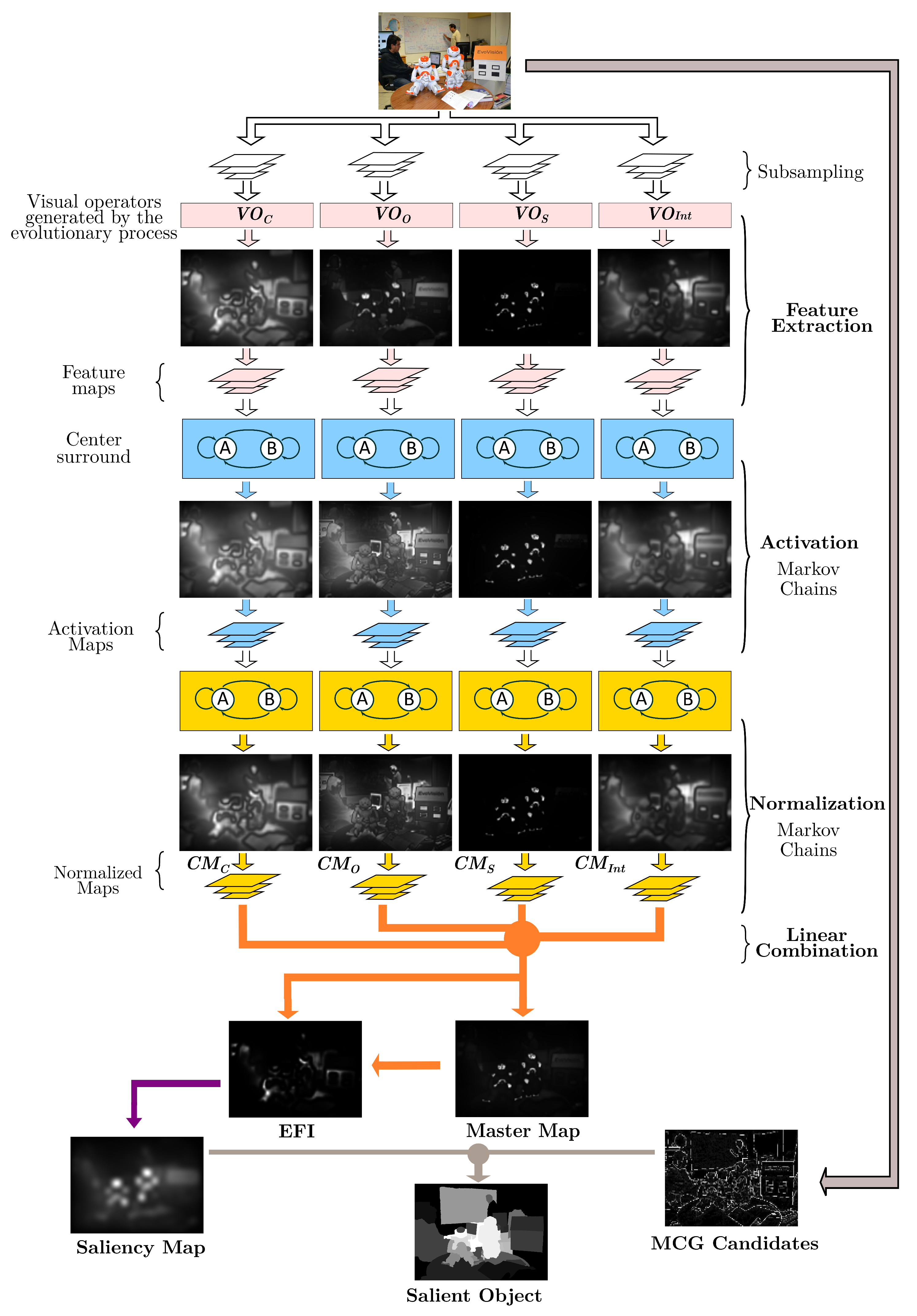
The idea of selecting these images highlights that we cannot blindly follow the statistical results without observing the outcomes. As we mentioned, FT is the most straightforward test. The mailbox is the object of interest, and we can agree that our proposed method, including the segmentation step, is slightly better than the others, but not without this crucial element. The following image provides an example of a questionable ground truth (the horse), which is not the most conspicuous object. None of the algorithms correctly identify the object. The last image provides an example of ground truth that we do not consider imprecise, but because the evaluation rests on the average, the ranking, in this case, is controversial. Note that even if the computer model is symbolic, the interpretation remains numeric and therefore, there exist computer errors. Nevertheless, the computation is data independent since the proposal follows a function-driven paradigm. Figure 5 illustrates the image processing through the whole GBVSBP+MCG program. The programs inserted in the template and provided in Table 18 are quite simple, helping in the overall explanation.
Figure 3. The precision–recall curve for FT, PASCAL-S, and IMGSAL datasets using the following algorithms: GBVSBP + MCG, SF, GBVS + MCG, PCAS, GC, FT, GBVSBP, and GBVS.
Applsci 12 10686 g003
Figure 4. Example of maps obtained in experiments whose results are controversial despite that our models observe better performance in the benchmark. The FT image shows the relevance of the segmentation process to rank highest in the benchmark. The PASCAL-S image shows a misleading ground truth that confuses all algorithms. Finally, the IMGSAL image shows a reasonably well-segmented image that contrasts with all others in the dataset, generating a controversial result.
Applsci 12 10686 g004
Next, we test our best solution (GBVSBP + MCG) on four databases studied in [6], and the results are in Table 20. Contreras-Cruz et al. designed the best solution, trained it with MSRA-A, then tested it with MSRA-BTest, ECSSD, SED2, and iCoseg. We observe that we scored highest on three datasets, MSRA-BTest, ECSSD, and iCoseg, while achieving competitive results on SED2. We provide such a comparison since [6] did not test their algorithms with the benchmark protocol. Therefore it is hard to make a clear comparison between both approaches, and the results we provide here illustrate the methodologies’ performance.
We provide a final set of experiments in Table 21 to illustrate the behavior of our evolutionary proposal in comparison with deep learning methodologies. Since such state-of-the-art methodologies run with small images, we run all experiments with images of 224 × 224 pixels, including our evolved GBVS, which does not have such limitations. As shown in Figure 4, GBVSBP + MCG is the best algorithm in our test against classic algorithms for FT and PASCAL-S, while GBVSBP is the best for IMGSAL. The results shown in these new experiments with IMGSAL exhibit its good performance against DHSNet and tying BASNet with a lower variance. Regarding FT, we observe that GBVSBP achieves the lowest score of all learning approaches. Nevertheless, according to Table 17, GBVSBP + MCG achieves a maximum score of 89.02, a value that is better than PiCANet and is between DHSNet and BASNet. Moreover, the results agree with those reported in Table 19, where DHSNet is better than GBVSBP but not compared to GBVSBP + MCG. Finally, the results with PASCAL-S show the poor performance of GBVSBP, but considering the expected improvement after combining it with the segmentation process, we could expect at least to overpass DHSNet as exemplified in the experiments provided in Figure 3, where the improvement was of more than 10 points. Beyond the statistical results, it is true that deep learning methods currently have the edge over other strategies, but most researchers take it for granted. As illustrated in this document, the community should include other approaches in the comparison, especially after considering other criteria, such as the robustness of SOD against adversarial attacks [45].
Figure 5. Brain programming result of the dorsal stream using the best GBVS + MCG program.
Applsci 12 10686 g005

5. Conclusions

In this work, we propose a method to improve the ADS model presented by [5]. This method consists of applying an algorithm called GBVS that surpasses Itti’s previous model. GBVS uses a graph-based approach using Markov chains while involving the same stages as the Itti model. Moreover, we follow the idea of combining fixation prediction with a segmentation algorithm to obtain a new method called GBVSBP + MCG to tackle the problem of salient object segmentation. As we show in the experiments, the novel design scores highest in the FT, IMGSAL, and PASCAL-S datasets of a benchmark provided by [30]. These tests show the strength and generalization power of the discovered model compared to others developed manually and current CNNs, such as DHSNet, which is surpassed by more than 12 percentage points in FT. We also give the results on four datasets described in [6] with outstanding results. The results are revealing regarding the difficulty of solving this visual task. In the FT and PASCAL-S, objects are defined with accurate ground truth, and the algorithm GBVSBP + MCG improves the results of the original algorithm slightly. However, in the IMGSAL database, the ground truth is poorly segmented, and GBVSBP significantly improves the score compared to the original proposal. Therefore, we can say that there is a considerable benefit in combining analytical methods with heuristic approaches. We believe that this mixture of strategies can help find solutions to challenging problems in visual computing and beyond. One advantage is that the overall process and final designs are explainable, which is considered a hot topic in today’s artificial intelligence. This research attempts to advance studies conducted by experts (neuroscientists, psychologists, and computer scientists) by adapting the symbolic paradigm for machine learning to find better ways of describing the brain’s inner workings.

Author Contributions

Conceptualization, G.O. and R.O.; Data curation, G.O., J.A.M.-C., M.O., A.O. and R.P.; Formal analysis, G.O., A.O. and G.I.-V.; Funding acquisition, G.O.; Investigation, G.O., J.A.M.-C., M.O., A.O., R.O. and R.P.; Methodology, G.O., J.A.M.-C. and R.P.; Project administration, G.O. and G.I.-V.; Resources, G.O., J.A.M.-C. and A.O.; Software, J.A.M.-C., M.O., A.O. and R.P.; Supervision, G.O.; Validation, G.O., J.A.M.-C., M.O., A.O., G.I.-V., R.O. and R.P.; Visualization, J.A.M.-C., M.O. and A.O.; Writing—original draft, G.O., J.A.M.-C., M.O. and A.O.; Writing—review and editing, G.O., G.I.-V. and R.O. All authors have read and agreed to the published version of the manuscript.

Funding

This research was funded by CICESE grant number 634-135.

Institutional Review Board Statement

Not applicable.

Informed Consent Statement

Not applicable.

Acknowledgments

The following project support this research: (1) Project titled “Estudio de la programación cerebral en problemas de reconocimiento a gran escala y sus aplicaciones en el mundo real” CICESE-634135. We want to thank the editorial office of applied sciences and Christine Zhang for approval of the full waiver of the article publishing charge.

Conflicts of Interest

The authors declare no conflict of interest.

Appendix A

In the present work, we integrate the GBVS algorithm into the ADS; since the functions were defined manually, we would like to incorporate learning. By evolving its dimensions, the BP paradigm enhanced the GBVS methodology with automated design capabilities. This nature-inspired technique, in turn, increased its performance by endowing it with the ability to learn, as shown in Figure 1.
In addition, we use the approach presented in [30], where the authors introduced a segmentation algorithm called MCG. The fusion of an optimized GBVS+MCG presents superior results if ground truth is accurate while testing object detection algorithms in the SOD benchmark.
As discussed in the previous chapter, the GBVS has several stages. As part of the integration with the BP, the GBVS underwent several changes. These transformations start with feature extraction, where two new color maps, HSV and CMYK, are extracted for each subsampling level.
The DKColor and Orientation dimensions are now dynamic, and a new dimension, ‘shape’, is added. The BP tree model comes into play, using the orientation subtree in the dimension of the same name, the DKColor dimension transforms to use the Color subtree, and finally, we add Form as a feature dimension through the shape subtree. A final transformation occurs later with a fourth subtree, charged with integrating features to the output as post-processing enhancement.
These changes allow GBVS to optimize its dimensions concerning image processing. This evolution of the GBVS also includes its merger with the MCG algorithm, which underwent a series of modifications.
Firstly, the segmentation mechanism and extraction of MCG characteristics are isolated, separating its operation from the flow of the evolutionary cycle. This division represents a saving of at least five times the time required, without loss in performance, by the MCG to process an image. We achieved this by storing each result in a file each time the image enters the evaluation of an individual generated by BP. We illustrate the execution times before and after its application below.
The time required for each image takes approximately 40 s (1 s for GBVS, 4 s for integration, and 35 for MCG) on average. A complete run requires 30 generations with 30 individuals to develop a solution, and each individual must process each of the images in the training set. In a hypothetical example with 120 images for training, there would be an execution time of
T = 30 30 120 40 = 4 , 860 , 000 s / 3600 = 1350 h / 24 = 56.25 days ,
and this time considers a single processing core.
Now, when studying the MCG algorithm, we realize that the output of each processed image does not change, and therefore it is not necessary to generate it more than once. We limit the processing of the images by the MCG to only once for each image, saving computational resources and improving the overall consumption by the evolutionary cycle. This idea brings as a consequence that with the same hardware components, the PC will only take the following time:
T = 120 35 = 3960 s / 3600 = 1.17 h ,
for 120 images, the available processing time would be
T = 30 30 120 5 = 540 , 000 s / 3600 = 150 h / 24 = 6.25 days ,
in total on average, representing an improvement of approximately 89% compared to the initial method. Since this work implies improvements in the functioning of the ADS model, it is necessary to explain in situ the changes we made to it. In this section, we describe the pseudocode algorithms of the brain programming of the new artificial dorsal route based on the one developed by [5].
We detail the evolutionary process in the Algorithm A1. We initialize GP variables between lines (1–6). The sets of functions and terminals of the three dimensions (orientation, color, and shape), and the function corresponding to the integration of features (7–14) are declared. Then we create the first generation of individuals in the population (15). In line 16, we initiate the reference list of training images. GP starts the cycle (17). The conditional if has a negative value only in the first loop; its function is to create a new generation from the current one (18–29).
After the pop individuals, we calculate their fitness—each fitness value is initialized to “0” (30). The cycle responsible for calculating aptitude begins (31). On line 32, the values of f i t n e s s c h r o m are initialized to “0”. The second cycle (33) begins, which is responsible for calculating the fitness of the individual whose index is i for each image in the list i m a g e s t r . To achieve this, executing the salobj_test_img (Algorithm A2) returns a proto-object (34). Then, this pro-object compares with the corresponding binary image (35), and the result corresponds to the fitness value of the individual i in the image j. We store results in f i t n e s s c h r o m , and at the end of the loop, the average of all fitness values is calculated (37). We preserve the individual with the best average fitness up to that moment at the end of each GP cycle (39).
The second cycle creates new generations of the population (18–29). The p a r e n t s c h r o m array (19) is emptied. Then (20) several individuals represented by pop_size and discriminated by a roulette selection method based on the fitness value of each individual in the population are assigned to p a r e n t s c h r o m . The higher the aptitude, the greater the chance of being selected. The array o f f s p r i n g c h r o m is also emptied (21), and a cycle is in charge of generating the new individuals from the parent individuals (22). The first step is to choose the genetic operation to perform through a roulette selection. The operations are chromosome-crossover, chromosome-mutation, gene-crossover, and gene-mutation. These genetic operators have a probability defined in the initialization (23). Genetic-crossover operators produce two child individuals from two parents, while mutation operators produce one child individual from the parent. We store these generated individuals in o f f s p r i n g c h r o m (25), and once the generation ends, these individuals replace those of the previous generation (27). Only the best individuals from a generation pass on to the next (28).
Algorithm A2 takes care of generating the proto-object. The first step is initializing the parameters necessary for executing the GBVS (1). Next, the salience map is obtained in gbvsResult (Algorithm A3) (2). This algorithm is responsible for using an individual generated by the GP to process the input image and convert it into a salience map and store it in salMap (3). The masks, candidate segments, segment numbers and MCG features are stored in masks, maskCCs, numSegs, mcg_feats respectively (Algorithm A4) (4). The previous algorithm segments the input image and generates an array of candidate segments according to the input image and the mode (second parameter) to accomplish it. This process consumes many resources, executed only once per image, and its result turns into a file for its next use. This strategy is possible because it always returns the same individual result for each image. The features and array indexes of the MCG masks are stored in curFeats, maskIdx respectively (4). This algorithm uses the GBVS bulge map and the segments generated by the MCG to highlight those segments that coincide with the most bulge areas of the GBVS map. On the next 2 lines, readjustments are made to the array data masks, mcg_feats (6–7). In the array allFeats, we store the features extracted from the MCG (8) for future computation. For the extraction of labels (labels) and their probabilities (probs), we apply a pre-trained tree model with saliency maps of the GBVS to the characteristics of the MCG (9). The labels are ordered from highest to lowest for later use (10). We reset the label index array in the next five lines (11–15). Next, the best masks of the MCG are extracted (16). In the next three lines, we execute rescaling processes and grayscale conversions of the final mask (17–19).
Algorithm A1 Evolving GBVS with BP
Purpose: Create a population of individuals. Each individual is made up of a minimum of 4 functions. The GBVS+MCG uses these functions, and the fitness function uses their results to determine the best individual.
Input:
  • num_gen: Number of cycles/generations in the evolutionary process.
  • pop_size: Number of individuals in the population.

Variables:
  • max_level: Maximum number of levels any tree can have.
  • max_trees: Number of trees (genes) that an individual (chromosome) must have.
  • prob_chrom_cross: Probability of applying a chromosome crossover.
  • prob_chrom_mut: Probability of applying a chromosome mutation.
  • pop: An array with all individuals in the population.
  • p a r e n t s c h r o m : A structure that saves the selected individuals as parents.
  • o f f s p r i n g c h r o m : An array that holds one or two new individuals, the product of some genetic operator applied to selected members of the current population.
  • new_pop: An array containing the individuals of the new population generation. It is the same size as pop.
  • p a r e n t s c h r o m : An array of image pairs used for training. The first is an RGB image, and the second is a binary image representing the RGB image’s proto-object.
  • i m a g e [ s t r ] : An array of image pairs used for training. The first is an RGB image, and the second is a binary image representing the RGB image’s proto-object.
  • fitness: An array that stores the average fitness values for each individual.
  • f i t n e s s c h r o m : An array that stores the fitness values of a single individual. f O , f C , f S , f F I : List of function sets regarding Orientation (O), Color (C), Shape (S), and Feature Integration (FI).
  • data_base_train: Number of cycles/generations in the evolutionary process.

Output:
  • best_ind: Save the individual with the best fitness value.
1:
max_level ← 9
2:
max_trees ← 4
3:
prob_chrom_cross ← 0.8
4:
prob_chrom_mut ← 0.2
5:
prob_gen_cross ← 0.8
6:
prob_gen_mut ← 0.2
7:
f O {Orientation functions}
8:
f C {Color Features}
9:
f S {Form Functions}
10:
f F I {Feature Integration Functions}
11:
t O {Orientation Terminals}
12:
t C {Color Terminals}
13:
t S {Form Terminals}
14:
t F I {Feature Integration Terminals}
15:
pop I n i t _ P o p ( f O , f C , f S , f F I , t O , t C , t S , t F I , p o p _ s i z e , m a x _ l e v e l , m a x _ t r e e s )
16:
i m a g e s t r Load(data_base_train)
17:
for (gen ← 1 to num_gen) do
18:
    if gen ≠ 1 then
19:
         p a r e n t s c h r o m .Clear()
20:
         p a r e n t s c h r o m Roulette(pop,fitness,pop.size)
21:
         o f f s p r i n g c h r o m .Clear()
22:
        while ( o f f s p r i n g c h r o m .length < p a r e n t s c h r o m .length) do
23:
           operator ← Roulette_Op(prob_chrom_cross,prob_chrom_mut,prob_gen_cross, prob_gen_mut)
24:
           i ← o f f s p r i n g c h r o m .length
25:
            o f f s p r i n g c h r o m .Add(Apply_Gen_Op(operator, p a r e n t s c h r o m ,i))
26:
        end while
27:
        pop ← o f f s p r i n g c h r o m
28:
        pop.Add(best_ind)
29:
    end if
30:
    fitness ← 0
31:
    for (i ← 1 to pop.length) do
32:
         f i t n e s s c h r o m 0
33:
        for (j ← 1 to i m a g e s t r .length ) do
34:
           proto ← salobj_test_img( i m a g e s t r [j,1],pop[i])
35:
            f i t n e s s c h r o m [j] ← Calc_Proto_Fitness(pop[i], i m a g e s t r [j,2])
36:
        end for
37:
        fitness[i] ← Mean( f i t n e s s c h r o m )
38:
    end for
39:
    best_ind ← Get_Best(pop, fitness, best_ind)
40:
end for
41:
return best_ind
Algorithm A2 salobj_test_img
Purpose
  • Proto-object generation.

Input
  • img: Image or image path.
  • param: Contains parameters for the algorithm.
  • forest: A pre-trained model for calculating the highest level characteristics. This model requires training the GBVS bulge maps or some other fixation prediction algorithm.
  • imgName: Name of the image to use.

Output
  • finalMask: Contains the proto-object.
1:
gbvsParam ← makeGBVSParams()
2:
gbvsResult ← gbvs_init(img, param.ind)
3:
salMap ← gbvsResult.master_map
4:
[masks,maskCCs,numSegs,mcg_feats] ← compute_mcg(img, ’accurate’, imgName, param)
5:
[curFeats, maskIdx] ← computeFeatures(maskCCs, salMap, [], param)
6:
masks ← masks(:,:,maskIdx)
7:
mcg_feats ← single(mcg_feats(maskIdx, :))
8:
allFeats ← [curFeats, mcg_feats]
9:
[labels, probs] ← forestApply(allFeats, forest)
10:
[labels, index] ← sort(labels, 1, ’descend’)
11:
sizeK ← param.topK
12:
if (sizeK > length(index)) then
13:
    sizeK ← length(index)
14:
end if
15:
index ← index(1:sizeK)
16:
topMasks ← masks(:,:,index)
17:
scores ← reshape((labels(index)/param.nbins), [1 1 sizeK])
18:
finalMask ← topMasks .* repmat(scores, [imgH, imgW, 1])
19:
finalMask ← mat2gray(sum(finalMask, 3))
20:
return finalMask
Algorithm A3 gbvs_init
Purpose
  • Configuration of initial parameters of the GBVS and its execution.

Input
  • img: Image or image path.
  • ind: Mathematical model generated by the BP.

Output
  • out: Contains the salience map.
1:
params ← makeGBVSParams
2:
params.channels ← ’DIOS’
3:
params.gaborangles ← [ 0, 45, 90, 135 ]
4:
params.levels ← 4
5:
params.tol ← 0.003
6:
params.salmapmaxsize ← round( max(size(img))/8 )
7:
params.ind ← ind
8:
params.gp ← 1
9:
params.shapeWeight ← 1
10:
out ← gbvs(img, params)
11:
return out
Algorithm A3 is in charge of initializing the execution parameters of the GBVS and executing it. The default parameters of the algorithm (1) are stored in param. Next, the channels (dimensions for the GP) to be used are chosen (2). The Gabor angles to use, the subsampling levels, the tolerance level of the eigenvector equilibrium mechanism, and the minimum subsampling size are established (3–6). The individual generated by the GP is also stored as well as the control variables and weights (7–9). Finally, we obtain the GBVS result for the input image (10).
Algorithm A4 compute_mcg
Purpose
  • Image segmentation and feature extraction.

Input
  • img: Image or image path.
  • mode: MCG execution mode.
  • imgName: Name of the image to use.
  • param: MCG execution parameters.

Output
  • masks: Contains the masks of the MCG conversions.
  • maskCCs: Contains the filtered masks of the MCG conversions.
  • numSegs: Number of parts in which the image is segmented.
  • mcg_feats: Contains the characteristics of the MCG result.
1:
if exist(char(strcat(’tmp/’,imgName,’.mat’)), ’file’) then
2:
    [masks,maskCCs,numSegs,mcg_feats] ← load(char(strcat(’tmp/’,imgName,’.mat’)))
3:
else
4:
    [candidates_mcg, mcg_feats] ← im2mcg_simple(img, mode)
5:
    mcg_feats ← mcg_feats(:, [1:3, 6:13, 15:16])
6:
    numProps ← size(candidates_mcg.scores, 1)
7:
    numProps ← min(numProps, param.maxTestProps)
8:
    masks ← false([size(img, 1), size(img, 2), numProps])
9:
    scores ← zeros([1 numProps])
10:
    sorted_scores ← candidates_mcg.scores
11:
    sorted_idx ← [1:numProps]
12:
    scores(1:numProps) ← sorted_scores(1:numProps)
13:
    sorted_idx ← sorted_idx(1:numProps)
14:
    mcg_feats ← [mcg_feats(sorted_idx, :), scores’]
15:
    props ← candidates_mcg.labels(sorted_idx)
16:
    for (curProp ← 1 to numProps) do
17:
        masks(:,:,curProp) ← ismember(candidates_mcg.superpixels, props{curProp})
18:
    end for
19:
    [masks, validMasks, maskCCs] ← filterMasks(masks, param.minArea)
20:
    mcg_feats ← mcg_feats(validMasks, :)
21:
    numSegs ← size(masks, 3)
save(char(strcat(’tmp/’,imgName,’.mat’)),’masks’,’maskCCs’,’numSegs’,’mcg_feats’)
22:
end if
23:
return [masks,maskCCs,numSegs,mcg_feats]
Algorithm A4 is in charge of converting the image into segments and characteristics of the MCG. Regarding the first two lines, the MCG verifies the existence of values corresponding to the image processing (1–2). This step is necessary to save the MCG time to process an image (approximately 30 s according to [30]). The MCG then processes the image to extract candidate segments and MCG features (4–6). The following five lines are used to process the MCG results (7–11). The scores and characteristics are readjusted (12–14) in the following three lines. Then the MCG results are converted into masks (15–18), filtered, and saved to a file (19–21). Finally, the masks, candidates, segment numbers, and features are returned (23).
Algorithm A5 is responsible for calculating the salience map of an image. Some constants necessary for executing the GBVS are established in the initial line, such as the weight matrix and the Gabor filters. This information is stored in a file for each image dimension to be processed and reused while keeping dimensions (1). In the following line, we extract the feature maps of the image. It is in this phase that the individual generated by the GP is used and stored param (Algorithm A6) (2). Then the activation maps are calculated for each feature map (3). These maps are then normalized (4). Next, each channel’s average of the feature maps is calculated (5). Next, the characteristics are added through the channels (6). Then the part of the individual corresponding to the integration of characteristics is added to the resulting salience map (33). This sum is blurred and finally returned (38).
Algorithm A6 extracts the features from the input image using the individual generated by the GP. In the initial line, an array is established with the subsampling levels of the image starting at two because one would be the image with the original dimensions. The next 11 lines of the algorithm are dedicated to the subsampling of the different channels of three color spaces (RGB, CMYK, and HSV) (2–12). In the array rawfeatmaps the feature maps of each of the channels are saved (orientation (Algorithm A7), color (Algorithm A8), shape (Algorithm A9) and intensity) for each of the levels (17). These maps result from applying the individual generated from the GP to each training image. Finally, these maps are returned (22).
Algorithm A7 is in charge of extracting the characteristics corresponding to the orientation channel. The subsampling index is stored in the initial line, which is then used to access the corresponding color channels for each level (1). The following 11 lines are used to store the different channels of the color spaces at each level that will be used later as terminals in evaluating the individual in the image (2–12). The result of this evaluation is stored and returned later (13–14).
Algorithm A8 is in charge of extracting the characteristics corresponding to the color. In the three initial lines, the three channels of the RGB color space of the input image (1–3) are regrouped. This channel also uses the DKL color space, which is obtained from the function rgb2dkl (4). In the following lines, this color space’s three channels are distributed (5–7). The subsampling index is assigned (8) to be then used to access the terminals that correspond to the channels of each color space used (11–20). The individual is then evaluated, stored, and returned (21–22).
Algorithm A9 is in charge of extracting the characteristics corresponding to the shape. The subsampling index is stored in the initial line, which is then used to access the corresponding color channels for each level (1). The following lines group together the three channels of the RGB color space of the input image (2–4). In the following seven lines, the channels of various color spaces are distributed (5–11). The individual is evaluated, stored, and then returned (21–22).
Algorithm A5 gbvs
Purpose
  • Compute the GBVS map of an image and place it in master_map.
  • If this image is part of a video sequence, motionInfo should be looped, and the information from the previous frame/image will be used if “flicker” or “motion” channels are used. It is necessary to initialize prevMotionInfo to [] for the first frame.

Input
  • ind: Individual resulting from the evolutionary cycle of the GP.
  • img: Image or image path.
  • (opcional) param: Contains parameters for the algorithm.

Output
  • master_map: It is the GBVS map for the image–resized it is the same size as the image.
  • feat_maps: Contains the final and normalized individual feature maps.
  • map_types: Contains a string description of each map in feat_map (respectively for each index).
  • intermed_maps: Contains all computed intermediate maps along the path (act. & norm.) used to compute feat_maps, which are then combined into master_map.
  • rawfeatmaps: It contains all the feature maps calculated at the different scales.
  • motionInfo: It contains information on the movement of the frames.
1:
[grframe,param] ← initGBVS(param,size(img))
2:
[rawfeatmaps,motionInfo] ← getFeatureMaps( img , param )
3:
allmaps ← getActivationMaps()
4:
norm_maps ← getNormalizationMaps()
5:
comb_norm_maps ← getCombinationNormalizationMaps()
6:
master_map ← getMasterMap()
7:
if (param.gp = 1) then
8:
    [R,G,B,image] ← mygetrgb( img )
9:
    image ← imresize( mean(image,3) , param.salmapsize , ’bicubic’)
10:
    R ← imresize( R , param.salmapsize , ’bicubic’)
11:
    G ← imresize( G , param.salmapsize , ’bicubic’)
12:
    B ← imresize( B , param.salmapsize , ’bicubic’)
13:
    [C,M,Y,K] ← rgb2cmyk(R,G,B)
14:
    C ← imresize( C , param.salmapsize , ’bicubic’)
15:
    M ← imresize( M , param.salmapsize , ’bicubic’)
16:
    Y ← imresize( Y , param.salmapsize , ’bicubic’)
17:
    K ← imresize( K , param.salmapsize , ’bicubic’)
18:
    [H,S,V] ← rgb2hsv(img)
19:
    H ← imresize( H , param.salmapsize , ’bicubic’)
20:
    S ← imresize( S , param.salmapsize , ’bicubic’)
21:
    V ← imresize( V , param.salmapsize , ’bicubic’)
22:
    dkl ← rgb2dkl( img )
23:
    dkl1 ← dkl(:,:,1)
24:
    dkl1 ← imresize( dkl1 , param.salmapsize , ’bicubic’)
25:
    dkl2 ← dkl(:,:,2)
26:
    dkl2 ← imresize( dkl2 , param.salmapsize , ’bicubic’)
27:
    dkl3 ← dkl(:,:,3)
28:
    dkl3 ← imresize( dkl3 , param.salmapsize , ’bicubic’)
29:
    conspicuity1 ← comb_norm_maps{1}
30:
    conspicuity2 ← master_map
31:
    conspicuity3 ← comb_norm_maps{3}
32:
    conspicuity4 ← comb_norm_maps{4}
33:
    master_map ← master_map + eval(param.ind.str(4))
34:
end if
35:
master_map ← attenuateBordersGBVS(master_map,4)
36:
master_map ← mat2gray(master_map)
37:
master_map ← getBluredMasterMap()
38:
return master_map
Algorithm A6 getFeatureMaps
Purpose
  • Extraction of feature maps.

Input
  • img: Image or image path.
  • param: Contains parameters for the algorithm.
  • prevMotionInfo: Information of the previous frame/image.

Output
  • rawfeatmaps: It contains all the feature maps calculated at different scales.
  • motionInfo: It contains information on the movement of the frames.
1:
levels ← [ 2 : param.maxcomputelevel ]
2:
imgL ← getIntensitySubsamples()
3:
imgR ← getRedSubsamples()
4:
imgG ← getGreenSubsamples()
5:
imgB ← getBlueSubsamples()
6:
imgC ← getCyanSubsamples()
7:
imgM ← getMagentaSubsamples()
8:
imgY ← getYellowSubsamples()
9:
imgK ← getKeySubsamples()
10:
imgH ← getHueSubsamples()
11:
imgS ← getSaturationSubsamples()
12:
imgV ← getBrightnessSubsamples()
13:
l ← 0
14:
for (i ← 1 to channels) do
15:
    for (j ← 1 to channels[i].numtypes ) do
16:
        for (k ← 1 to levels ) do
17:
           rawfeatmaps[l] ← channelfunc(param,imgLk,imgRk,imgGk,imgBk,ti)
18:
           l ← l + 1
19:
        end for
20:
    end for
21:
end for
22:
return rawfeatmaps
Algorithm A7 OrientationGP
Purpose
  • Feature extraction from the orientation channel.

Input
  • fparam: Channel execution parameters.
  • img: Image subsampled with intensity values.
  • imgR: Red channel of the subsampled image.
  • imgG: Green channel of the subsampled image.
  • imgB: Blue channel of the subsampled image.
  • typeidx: Image subsampling rate.

Output
  • out: It contains the characteristics map of the orientation channel.
1:
n ← typeidx
2:
R ← imgR
3:
G ← imgG
4:
B ← imgB
5:
C ← fparam.terminals(n).C
6:
M ← fparam.terminals(n).M
7:
Y ← fparam.terminals(n).Y
8:
K ← fparam.terminals(n).K
9:
H ← fparam.terminals(n).H
10:
S ← fparam.terminals(n).S
11:
V ← fparam.terminals(n).V
12:
imagen ← fparam.terminals(n).V
13:
out.map ← eval(fparam.ind.str(1))
14:
return out
Algorithm A8 dkColorGP
Purpose
  • Extraction of characteristics of the channel of the form.

Input
  • fparam: Channel execution parameters.
  • img: Image subsampled with intensity values.
  • imgR: Red channel of the subsampled image.
  • imgG: Green channel of the subsampled image.
  • imgB: Blue channel of the subsampled image.
  • typeidx: Image subsampling rate.

Output
  • out: Contains the feature map of the shape channel.
1:
rgb ← repmat( imgR , [ 1 1 3 ] )
2:
rgb(:,:,2) ← imgG
3:
rgb(:,:,3) ← imgB
4:
dkl ← rgb2dkl( rgb )
5:
dkl1 ← dkl(:,:,1)
6:
dkl2 ← dkl(:,:,2)
7:
dkl3 ← dkl(:,:,3)
8:
n ← typeidx
9:
image ← []
10:
image ← img
11:
R ← imgR
12:
G ← imgG
13:
B ← imgB
14:
C ← fparam.terminals(n).C
15:
M ← fparam.terminals(n).M
16:
Y ← fparam.terminals(n).Y
17:
K ← fparam.terminals(n).K
18:
H ← fparam.terminals(n).H
19:
S ← fparam.terminals(n).S
20:
V ← fparam.terminals(n).V
21:
out.map ← eval(fparam.ind.str(2))
22:
return out
Algorithm A9 ShapeGP
Purpose
  • Color channel feature extraction.

Input
  • fparam: Channel execution parameters.
  • img: Image subsampled with intensity values.
  • imgR: Red channel of the subsampled image.
  • imgG: Green channel of the subsampled image.
  • imgB: Blue channel of the subsampled image.
  • typeidx: Image subsampling rate.

Output
  • out: Contains the Color channel feature map.
1:
n ← typeidx
2:
R ← imgR
3:
G ← imgG
4:
B ← imgB
5:
C ← fparam.terminals(n).C
6:
M ← fparam.terminals(n).M
7:
Y ← fparam.terminals(n).Y
8:
K ← fparam.terminals(n).K
9:
H ← fparam.terminals(n).H
10:
S ← fparam.terminals(n).S
11:
V ← fparam.terminals(n).V
12:
out.map ← eval(fparam.ind.str(3))
13:
return out

References

  1. Ndayikengurukiye, D.; Mignotte, M. Salient object detection by LTP texture characterization on opposing color pairs under slico superpixel constraint. J. Imaging 2022, 8, 110. [Google Scholar] [CrossRef]
  2. Ahmed, K.; Gad, M.A.; Aboutabl, A.E. Performance evaluation of salient object detection techniques Multimed. Tools Appl. 2022, 81, 21741–21777. [Google Scholar] [CrossRef]
  3. Gupta, A.K.; Seal, A.; Khanna, P.; Yazidi, A.; Krejcar, O. Gated contextual features for salient object detection. IEEE Trans. Instrum. Meas. 2021, 70, 1–13. [Google Scholar] [CrossRef]
  4. Gupta, A.K.; Seal, A.; Khanna, P.; Krejcar, O.; Yazidi, A. Awks: Adaptive, weighted k-means-based superpixels for improved saliency detection. Pattern Anal. Appl. 2021, 24, 625–639. [Google Scholar] [CrossRef]
  5. Dozal, L.; Olague, G.; Clemente, E.; Hernández, D.E. Brain programming for the evolution of an artificial dorsal stream. Cogn. Comput. 2014, 6, 528–557. [Google Scholar] [CrossRef]
  6. Contreras-Cruz, M.A.; Martinez-Rodriguez, D.E.; Hernandez-Belmonte, U.H.; Ayala-Ramirez, V. A genetic programming framework in the automatic design of combination models for salient object detection. Genet. Program. Evolvable Mach. 2019, 20, 285–325. [Google Scholar] [CrossRef]
  7. Clemente, E.; Olague, G.; Dozal, L.; Mancilla, M. Object recognition with an optimized ventral stream model using genetic programming. In Lecture Notes in Computer Science (Including Subseries Lecture Notes in Artificial Intelligence and Lecture Notes in Bioinformatics); Springer: Berlin/Heidelberg, Germany, 2012; Volume 7248, pp. 315–325. [Google Scholar]
  8. Olague, G.; Clemente, E.; Hernandez, D.E.; Barrera, A.; Chan-Ley, M.; Bakshi, S. Artificial visual cortex and random search for object categorization. IEEE Access 2019, 7, 54054–54072. [Google Scholar] [CrossRef]
  9. Rojas-Quintero, J.; Rodríguez-Liñán, M. A literature review of sensor heads for humanoid robots. Robot. Auton. Syst. 2021, 143, 103834. [Google Scholar] [CrossRef]
  10. Treisman, A.M.; Gelade, G. A feature-integration theory of attention. Cogn. Psychol. 1980, 12, 97–136. [Google Scholar] [CrossRef]
  11. Khan, A.; Qureshi, A.S.; Wahab, N.; Hussain, M.; Hamza, M.Y. A recent survey on the applications of genetic programming in image processing. Comput. Intell. 2021, 37, 1745–1778. [Google Scholar] [CrossRef]
  12. Mohammed, G.S.; Al-Janabi, S. An innovative synthesis of optmization techniques (FDIRE-GSK) for generation electrical renewable energy from natural resources. Results Eng. 2022, 16, 100637. [Google Scholar] [CrossRef]
  13. Olague, G.; Olague, M.; Ibarra-Vazquez, G.; Reducindo, I.; Barrera, A.; Martinez, A.; Briseno, J.L. Modelling Hierarchical Architectures with Genetic Programming and Neuroscience Knowledge for Image Classification through Inferential Knowledge. In Genetic Programming Theory and Practice XIX; Springer: Berlin/Heidelberg, Germany, 2023. [Google Scholar]
  14. Al-Janabi, S.; Alkaim, A. A novel optimization algorithm (lion-ayad) to find optimal dna protein synthesis. Egypt. Inform. J. 2022, 23, 271–290. [Google Scholar] [CrossRef]
  15. Gupta, A.K.; Seal, A.; Khanna, P.; Herrera-Viedma, E.; Krejcar, O. Almnet: Adjacent layer driven multiscale features for salient object detection. IEEE Trans. Instrum. Meas. 2021, 70, 1–14. [Google Scholar] [CrossRef]
  16. Olague, G. Evolutionary Computer Vision: The First Footprints; Springer: Berlin/Heidelberg, Germany, 2016. [Google Scholar]
  17. Santamaría, J.; Rivero-Cejudo, M.L.; Martos-Fernández, M.A.; Roca, F. An overview on the latest nature-inspired and metaheuristics-based image registration algorithms. Appl. Sci. 2020, 10, 1928. [Google Scholar] [CrossRef] [Green Version]
  18. Iqbal, M.; Naqvi, S.S.; Browne, W.N.; Hollitt, C.; Zhang, M. Learning feature fusion strategies for various image types to detect salient objects. Pattern Recognit. 2016, 60, 106–120. [Google Scholar] [CrossRef]
  19. Ibarra-Vazquez, G.; Olague, G.; Chan-Ley, M.; Puente, C.; Soubervielle-Montalvo, C. Brain programming is immune to adversarial attacks: Towards accurate and robust image classification using symbolic learning. Swarm Evol. Comput. 2022, 71, 101059. [Google Scholar] [CrossRef]
  20. Perez-Cham, O.E.; Puente, C.; Soubervielle-Montalvo, C.; Olague, G.; Aguirre-Salado, C.A.; Nuñez-Varela, A.S. Parallelization of the honeybee search algorithm for object tracking. Appl. Sci. 2020, 10, 2122. [Google Scholar] [CrossRef] [Green Version]
  21. Perez-Cham, O.E.; Puente, C.; Soubervielle-Montalvo, C.; Olague, G.; Castillo-Barrera, F.-E.; Nunez-Varela, J.; Limon-Romero, J. Automata design for honeybee search algorithm and its applications to 3d scene reconstruction and video tracking. Swarm Evol. Comput. 2021, 61, 100817. [Google Scholar] [CrossRef]
  22. Pillay, N.; Qu, R. (Eds.) Automated Design of Machine Learning and Search Algorithms; Springer: Berlin/Heidelberg, Germany, 2021. [Google Scholar] [CrossRef]
  23. Creel, K.A. Transparency in complex computational systems. Philos. Sci. 2020, 87, 1–37. [Google Scholar] [CrossRef]
  24. Li, N.; Bi, H.; Zhang, Z.; Kong, X.; Lu, D. Performance comparison of saliency detection. Adv. Multimed. 2018, 2018, 1–13. [Google Scholar] [CrossRef]
  25. Borji, A.; Cheng, M.-M.; Hou, Q.; Jiang, H.; Li, J. Salient object detection: A survey. Comput. Vis. Media 2019, 5, 117–150. [Google Scholar] [CrossRef] [Green Version]
  26. Gupta, A.K.; Seal, A.; Prasad, M.; Khanna, P. Salient object detection techniques in computer vision—A survey. Entropy 2020, 22, 1174. [Google Scholar] [CrossRef] [PubMed]
  27. Wang, W.; Lai, Q.; Fu, H.; Shen, J.; Ling, H.; Yang, R. Salient object detection in the deep learning era: An in-depth survey. IEEE Trans. Pattern Anal. Mach. Intell. 2021, 44, 3239–3259. [Google Scholar] [CrossRef]
  28. Borji, A.; Sihite, D.N.; Itti, L. Salient object detection: A benchmark. In Lecture Notes in Computer Science (Including Subseries Lecture Notes in Artificial Intelligence and Lecture Notes in Bioinformatics); Springer: Berlin/Heidelberg, Germany, 2012; Volume 7573, pp. 414–429. [Google Scholar]
  29. Borji, A.; Cheng, M.; Jiang, H.; Li, J. Salient object detection: A benchmark. IEEE Trans. Image Process. 2015, 24, 5706–5722. [Google Scholar] [CrossRef] [Green Version]
  30. Li, Y.; Hou, X.; Koch, C.; Rehg, J.M.; Yuille, A.L. The secrets of salient object segmentation. In Proceedings of the IEEE Computer Society Conference on Computer Vision and Pattern Recognition, Columbus, OH, USA, 23–28 June 2014; pp. 280–287. [Google Scholar]
  31. Liu, N.; Han, J. Dhsnet: Deep hierarchical saliency network for salient object detection. In Proceedings of the 2016 IEEE Conference on Computer Vision and Pattern Recognition (CVPR), Las Vegas, NV, USA, 27–30 June 2016; pp. 678–686. [Google Scholar]
  32. Xuebin, X.; Zhang, Z.; Huang, C.; Hao, C.; Dehghan, M.; Jagersand, M. BASNet: Boundary-aware Salient Object Detection. In Proceedings of the IEEE/CVF Conference on Computer Vision and Pattern Recognition (CVPR), Long Beach, CA, USA, 15–20 June 2019; pp. 7471–7481. [Google Scholar]
  33. Liu, N.; Han, J.; Yang, M.-H. PiCANet: Learning Pixel-wise Contextual Attention for Saliency Detection. In Proceedings of the IEEE/CVF Conference on Computer Vision and Pattern Recognition (CVPR), Salt Lake City, UT, USA, 18–23 June 2018; pp. 3089–3098. [Google Scholar]
  34. Koch, C.; Ullman, S. Shifts in selective visual attention: Towards the underlying neural circuitry. In Human Neurobiology; Springer: Berlin/Heidelberg, Germany, 1985; Volume 4, pp. 219–227. [Google Scholar]
  35. Itti, L.; Koch, C.; Niebur, E. A model of saliency-based visual attention for rapid scene analysis. IEEE Trans. Pattern Anal. Mach. Intell. 1998, 20, 1254–1259. [Google Scholar] [CrossRef] [Green Version]
  36. Olague, G.; Hernandez, D.E.; Clemente, E.; Chan-Ley, M. Evolving head tracking routines with brain programming. IEEE Access 2018, 6, 26254–26270. [Google Scholar] [CrossRef]
  37. Olague, G.; Hernández, D.E.; Llamas, P.; Clemente, E.; Brise no, J.L. Brain programming as a new strategy to create visual routines for object tracking: Towards automation of video tracking design. Multimed. Tools Appl. 2019, 78, 5881–5918. [Google Scholar] [CrossRef]
  38. Harel, J.; Koch, C.; Perona, P. Graph-based visual saliency. In Advances in Neural Information Processing Systems; Mit Press: Cambridge, MA, USA, 2007; pp. 545–552. [Google Scholar]
  39. Clemente, E.; Chavez, F.; Fernandez De Vega, F.; Olague, G. Self-adjusting focus of attention in combination with a genetic fuzzy system for improving a laser environment control device system. Appl. Soft Comput. J. 2015, 32, 250–265. [Google Scholar] [CrossRef]
  40. Everingham, M.; Gool, L.V.; Williams, C.K.I.; Winn, J.; Zisserman, A. The pascal visual object classes (voc) challenge. Int. J. Comput. Vis. 2010, 88, 303–338. [Google Scholar] [CrossRef]
  41. Perazzi, F.; Krahenbuhl, P.; Pritch, Y.; Hornung, A. Saliency filters: Contrast based filtering for salient region detection. In Proceedings of the IEEE Computer Society Conference on Computer Vision and Pattern Recognition, Providence, RI, USA, 16–21 June 2012; pp. 733–740. [Google Scholar]
  42. Margolin, R.; Tal, A.; Zelnik-Manor, L. What makes a patch distinct? In Proceedings of the 2013 IEEE Conference on Computer Vision and Pattern Recognition, Portland, OR, USA, 23–28 June 2013; pp. 1139–1146. [Google Scholar]
  43. Cheng, M.M.; Zhang, G.X.; Mitra, N.J.; Huang, X.; Hu, S.M. Global contrast based salient region detection. In Proceedings of the IEEE Computer Society Conference on Computer Vision and Pattern Recognition, Colorado Springs, CO, USA, 20–25 June 2011; pp. 409–416. [Google Scholar]
  44. Achantay, R.; Hemamiz, S.; Estraday, F.; Süsstrunky, S. Frequency-tuned salient region detection. In Proceedings of the 2009 IEEE Computer Society Conference on Computer Vision and Pattern Recognition Workshops, CVPR Workshops 2009, Miami, FL, USA, 20–25 June 2009; Volume 2009, pp. 1597–1604. [Google Scholar]
  45. Pineda, R.; Olague, G.; Ibarra-Vazquez, G.; Martinez, A.; Vargas, J.; Reducindo, I. Brain Programming and Its Resilience Using a Real-World Database of a Snowy Plover Shorebird. In International Conference on the Applications of Evolutionary Computation (Part of EvoStar), EvoApplications; Springer: Cham, Switzerland, 2022; pp. 603–618. [Google Scholar]
Figure 2. Brain programming statistics of the run corresponding to the best GBVSBP model for the FT database. We observe the convergence of fitness, diversity of solutions, number of nodes, and depth of solutions. It seems that the total number of generations can be reduced to 15.
Applsci 12 10686 g002
Table 9. Performance of the best individuals of the GBVSBP + MCG model for all FT database runs. Each pair of training and testing corresponds to one experiment of the k-fold. Therefore, we obtain 30 executions of our system and report the standard deviation for each run set.
FT Database
FoldRun 1Run 2Run 3Run 4Run 5Run 6
TrngTestTrngTestTrngTestTrngTestTrngTestTrngTest
193.3992.9093.6293.0993.6793.3593.2994.1493.5592.1993.2793.44
294.5386.6794.0286.1293.7584.6193.7386.6793.8086.8493.7485.38
392.8493.5592.8292.7692.6992.2293.0594.3692.4592.7892.6392.90
493.3392.7792.8693.6492.7693.5492.9891.5992.8793.8993.2390.62
593.2592.8693.4595.0693.0294.3193.2092.2293.0393.3193.0092.18
Average93.4791.7593.3592.1393.1891.6193.2591.8093.1491.8093.1790.90
σ 0.632.860.513.480.503.980.293.110.542.840.413.26
Table 10. Program structure of the operators corresponding to the best solution for the FT database. We select this solution from the 30 executions of Table 9. The final solution is more complex than the previous experiments. Still, the program is interpretable. The first visual operator applies a filter, while the second computes two times the complement of D K L r . Then, the shape operator applies a multiplication between bottom-hat operations to I b . Finally, the feature integration uses filters and derivatives to the conspicuity maps using algebraic operations.
   EVO d and EFI OperatorsFitness
   E V O O = G σ = 1 ( I m ) Training = 0.9453
   E V O C = C o m p l e m e n t ( C o m p l e m e n t ( D K L r ) ) Testing = 0.9506
   E V O S = ( ( b o t t o m h a t ( I b ) × ( b o t t o m h a t ( I b ) )
   E F I = | ( G ( σ = 1 ) ( C M M M ) × 0.63 ) + ( ( D y ( D y ( C M C ) ) D y ( D y ( C M M M ) ) ) D y ( D y ( C M M M ) ) ) |
Table 11. Performance of the best individuals of the GBVSBP model for all FT database runs. Each pair of training and testing corresponds to one experiment of the k-fold. Therefore, we obtain 30 executions of our system and report the standard deviation for each run set.
FT
FoldRun 1Run 2Run 3Run 4Run 5Run 6
TrngTestTrngTestTrngTestTrngTestTrngTestTrngTest
171.2771.9470.2370.3972.0472.2370.7370.9971.2270.8072.5973.65
270.0063.0567.0465.7368.6668.8667.5769.0169.566.5868.1867.78
371.7164.8271.8167.9271.1668.1571.2264.1572.1468.0271.0866.86
469.2373.4570.6966.1371.3268.1168.1573.8168.7771.1370.8769.42
568.0867.6868.5267.2068.8866.0369.3864.2569.1768.1968.7367.59
Average70.0668.1969.6667.4770.4168.6869.4168.4470.0768.9470.2969.06
σ 1.484.471.881.851.542.251.584.231.511.951.812.73
Table 18. Program structure of the operators corresponding to the best solution for the FT database. We select this solution from the seven executions of Table 17. Note that we can simplify the second tree. However, we report the programs as returned by the computer.
   EVO d and EFI OperatorsFitness
   E V O O = G ( σ = 1 ) ( D y ( I y ) ) Training = 0.8902
   E V O C = ( ( D K L Φ 1 / 0.62 ) ( ( ( E x p ( I b ) 1 / 0.62 ) 1 / 0.62 ) ( ( D K L Φ D K L Φ ) ( I b I b ) ) ) ) Testing = 0.8856
   E V O S = I y
   E F I = C M M M
Table 19. Comparison using the benchmark with other algorithms in the FT database [30]. This ranking of solutions applies a set of images separated from the rest of the photos as a challenging test. The evolved solution improves the original proposal and defeats DHSNet by a large margin.
Saliency ModelScore (F-Measure)
GBVSBP + MCG86.72
SF [41]85.38
GBVS + MCG [30]85.33
PCAS [42]83.93
GC [43]80.64
DHSNet [6]74.06
FT [44]71.23
GBVSBP69.08
GBVS [30]65.25
FOA [5]60.05
Table 20. Comparison with others models and databases published in [6]. Our proposal achieves better results than the more complex proposal using compound functions.
DatasetGAPSOGPMCCGPSEDGBVSBP + MCG
MSRA-BTest0.75790.74550.77110.76620.8308
ECSSD0.62000.59880.65920.65920.7591
SED20.69140.67010.71480.73400.6919
iCoseg0.66780.65570.68650.71570.7168
Table 21. Testing BP with GBVS against deep learning models for all databases. Since we are not combining the best programs with the segmentation step, the results are less performing for FT and PASCAL-S. However, this strategy is better for IMGSAL, as explained earlier. In general, we can say that the proposal is competitive compared to deep learning.
Datasets
AlgorithmFTIMGSALPASCAL-S
Avg. σ Avg. σ Avg. σ
BP73.8412.4862.6623.9662.9420.89
BASNet92.6712.5163.7531.7380.2021.15
PiCANet81.4515.2771.6022.1675.8119.80
DHSNet88.6312.4353.6324.8568.1421.03
Publisher’s Note: MDPI stays neutral with regard to jurisdictional claims in published maps and institutional affiliations.