Article

Prediction of Flight Delays at Beijing Capital International Airport Based on Ensemble Methods

College of Civil Aviation, Nanjing University of Aeronautics and Astronautics, Nanjing 211106, China
*
Author to whom correspondence should be addressed.
Appl. Sci. 2022, 12(20), 10621; https://doi.org/10.3390/app122010621
Submission received: 9 September 2022 / Revised: 12 October 2022 / Accepted: 17 October 2022 / Published: 20 October 2022
(This article belongs to the Special Issue Analysis, Optimization, and Control of Air Traffic System)

Abstract

:
Predicting flight delays plays a critical role in reducing financial losses and increasing passenger satisfaction. Due to their ability to combine multiple algorithms, ensemble methods have demonstrated strong predictive performance in many research fields. In this paper, ensemble methods are adopted to predict flight delays. First, based on the current studies, two novel explanatory variables, named arrival/departure pressure and cruise pressure, are proposed as factors affecting flight delays. Second, we introduce the ensemble methods and select representative algorithms for the prediction problem. In addition to the ensemble methods, classical algorithms are also used to predict flight delays. Finally, the actual operational data of Beijing Capital International Airport were utilized to conduct a case study. The results show that the stacking method has better prediction performance than other baseline methods. The mean absolute error (MAE) of the stacking method was about 12.58 min on the test dataset. Furthermore, we tested the effect of the two explanatory variables proposed in this paper, and the results show that the MAE was reduced by about 20% by using the stacking method.

1. Introduction

In recent years, with the increasing demand for air traffic, air traffic systems from home and abroad have been under tremendous pressure, resulting in serious flight delays. According to the Civil Aviation Administration of China (CAAC), the punctuality rate for passenger flights nationwide was 81.65% in 2019 [1]. Meanwhile, according to the U.S. Bureau of Transportation Statistics, the punctuality rate for major U.S. airlines was only 79.99% during the same period [2]. Predicting flight delays is crucial for airports, airlines, and passengers. More delayed flights mean more stranded passengers, resulting in airport congestion. If flight delays can be predicted and monitored in advance, airports can take appropriate and timely plans to prevent the cascading effect from affecting the normal operation of the airport. Airlines can notify passengers of potential flight delays in advance to ease their stress, reduce complaint rates, and increase passenger satisfaction. Passengers can plan their travel flexibly to reduce financial and time losses. Moreover, delays and atmospheric pollution, noise, accidents, and traffic congestion are the main environmental influences of the transportation industry [3].
COVID-19 created an unprecedented crisis for airlines worldwide, resulting in a reduction in the number of commercial flights [4]. Thus, flight delays also dropped. For example, the average delay for passenger flights across China in 2020 was 9 min, a decrease of 5 min year-on-year [1]. However, with the recovery from the epidemic, the demand for air traffic has maintained strong growth momentum. Therefore, prediction of flight delays will remain an important topic in the future.
With the rapid advancement of smart airport construction, the civil aviation industry has put forward higher requirements for data support. Currently, airports are already equipped with many intelligent systems for storing operational data, such as Airport Operational Databases (AODBs). These databases provide strong support for flight delay predictions. Many methods have been adopted, based on historical operation data, including the econometric model [5], historical data regression [6], and Bayesian network [7]. As machine learning (ML) continues to evolve, more and more researchers are applying it to air traffic, including random forest (RF) [8], support vector regression (SVR) [9], and recurrent neural networks (RNNs) [10]. In recent years, ensemble methods, as a branch of ML, have been applied to study the travel times of vehicles and buses and the estimated time of arrival of flights [11,12,13]. To improve prediction performance, ensemble methods combine several weak learners into a strong learner, a method which is applicable in the study of predicting flight delays.
Previous researchers have mainly considered macro factors in their models, including weather, laws of delay propagation, and delay causality [14]. We call these macro factors because their impact on delays is not real-time and can only be observed over a long period. Due to difficulties of quantification, more specific micro factors such as airport congestion and route congestion are often ignored. However, these micro factors can have a direct impact on flight delays, and can play an important role in real-time or short-term advance prediction. Therefore, in this paper we propose two novel explanatory variables, named arrival/departure pressure and cruise pressure, for use along with macro factors in prediction of flight delays, and explore their effect within models. In terms of variable processing, previous studies have tended to use the one-hot encoding method for temporal data, including hours of the day, days of the week, and months in a year. However, this type of encoding ignores the unique periodicity of temporal data. Therefore, to retain periodicity, we adopted the sine and cosine functions to convert the temporal data to (x, y) coordinates on a circle, and explored the impact of this encoding method on prediction performance.
The main contributions of this paper can be summarized as follows: (1) We applied stacking methods, a type of ensemble technique, to build a model that can reject poorer-performing models and highlight the best-performing ones. (2) We propose new explanatory variables, called arrival/departure pressure and cruise pressure, to describe congestion in the airport and the air-route situation. (3) We combined macro and micro factors as explanatory variables for prediction, which can improve prediction accuracy. (4) To preserve periodicity, we encoded the temporal data using sine and cosine functions. (5) To verify the effectiveness of the model, we used the actual departure flight data of Beijing Capital International Airport (PEK) for one year.
The rest of the paper is organized as follows: Section 2 describes related works. Section 3 discusses the methodology and model used in this paper. Section 4 provides a case study, including data description and preprocessing, variable selection, and algorithms. Finally, the results and discussion are described in Section 5 and the conclusion is presented in Section 6.

2. Related Works

Earlier studies used statistical modeling methods to estimate the probability of flight delays. For example, Hsiao et al. [5] developed an econometric model for estimating average daily delays. Tu et al. [6] decomposed delays into three patterns (propagation, seasonal, and random patterns), and proposed an estimation algorithm for flight-departure delay. However, the accuracy of the results obtained by the above methods was low, and they are infrequently applied in practice. Unlike the above studies, the current study proposes a practical flight-delay prediction model that aims to reduce problems such as airport congestion by accurately predicting the delay of each flight.
ML has been widely used for flight-delay prediction. Choi et al. [15] predicted airline delays caused by inclement weather conditions using decision trees, RF, AdaBoost, and K-nearest neighbor (KNN). They gathered flight schedules and weather forecasts to predict whether a scheduled flight would be delayed or on time. In addition to the binary classification of predicting whether or not a flight would be delayed, certain delay thresholds have been set. Rebollo et al. [8] set three delay thresholds (45, 60, and 90 min), and used RF to predict departure delays 2 to 4 h ahead. Gui et al. [16] set up dichotomous, trichotomous, and quadruple classification problems according to different delay thresholds. They implemented RF-based and long short-term memory (LSTM)-based architectures to predict individual flight delays. Stefanovič et al. [17] divided flight time deviation into six intervals and used seven supervised learning algorithms including RF, SVM, and decision trees to predict time deviation of flights at Lithuanian airports. Because a specific delay-prediction value is more in line with the needs of passengers, airlines, and airports, many scholars have attempted to predict the specific delay values of flights and airports. Ye et al. [18] predicted hourly aggregate flight-departure delays at Nanjing Lukou International Airport (NKG), using supervised learning methods. Guo et al. [19] proposed a hybrid method of random forest regression and maximal information coefficient (RFR-MIC) for delay prediction.
Deep learning (DL) is a new research direction in the field of ML, involving increasingly complex model structures. Many scholars have introduced it to flight-delay prediction. Yu et al. [20] employed a deep belief network to predict flight delays. Zeng et al. [21] proposed a deep graph-embedded LSTM (DGLSTM) model to predict delays at 325 airports in the United States. Bao et al. [22] developed a novel graph-to-sequence learning architecture with attention mechanism (AG2S-Net) to predict hourly delays in the airport network from multiple steps ahead. Cai et al. [23] proposed a flight-delay prediction approach based on a graph convolutional neural network (GCN), from an airport network perspective. Most of the above studies predicted average hourly delays in airports from the perspective of airport networks. However, passengers and airlines are more concerned with specific delays to individual flights. Therefore, in this study, we used data from PEK to Hangzhou International Airport (HGH) as a case study, to predict specific delays for each flight on this route.
As shown in Table 1, few studies have considered micro factors that can have a direct impact on flight delays. Although other factors such as weather and temporal data have an impact on flight delays, this impact is not immediate and requires a large amount of data to summarize. Therefore, the current study combined macro and micro factors, defining arrival/departure pressure and cruise pressure to predict specific delays for flights on a single route. To improve prediction performance, we applied ensemble methods that can form strong learners by combining several weak learners, and tested their effectiveness using a dataset obtained from CAAC.

3. Methodology

3.1. Ensemble Methods

Ensemble methods use multiple models to obtain better performance. Conventional ensemble methods include bagging, boosting, and stacking methods [24].

3.1.1. Bagging Methods

The basis of bagging methods is the use of the bootstrap sampling method to obtain T data subsets each containing m training samples to separately train the base learner. For the dataset D , one sample is randomly selected and added to the data subset, and then returned to the dataset D . This is conducted a total of m times. After repeating the operation T times, we obtain T data subsets, each containing m samples. Some samples in the dataset D may appear several times in the data subsets, and some may never appear.
The RF algorithm is a special kind of bagging method. The base learners of the RF algorithm are provided by the classification and regression trees (CART) model, and random attribute selection is introduced in the CART training process.

3.1.2. Boosting Methods

Boosting methods employ a serial working mechanism, dependent on the training of individual learners, performed serially step by step. First, a base learner is trained by the dataset D 1 . Then, the weight of samples with low prediction accuracy is increased. The adjusted dataset D 2 is utilized to train the next base learner. The operation is repeated T times to generate the ensemble learner, by weighting T base learners.
The most famous and widely used boosting method is the AdaBoost algorithm. The AdaBoost algorithm uses exponential loss function, so the update of weights and sample distribution revolves around minimizing the exponential loss function.

3.1.3. Stacking Methods

Stacking is an ensemble learning method [24]. The model has two layers, the first consisting of multiple base learners and the second being a single learner, called the meta-learner. Base learners consist of different types of learners with high performance. The meta-learner should be a relatively simple machine-learning model, to avoid overfitting.

3.2. Explanatory Variables

In this section, we introduce the explanatory variables that may affect flight delays.

3.2.1. Flight Attributes

(1)
Airline properties
Airports have different priorities and resource allocations for different airlines. Airline bases are the airports where an airline has its hubs. Airlines often select certain airports as bases that serve as hubs, where their flights can stay overnight. Airline properties consist of two factors, i.e., the airline and whether the airport is used as a base.
(2)
Aircraft capacity
Larger aircraft typically take up more airport resources and are given priority in takeoff and landing. Therefore, aircraft capacity is considered a potential factor affecting flight delays. The number of aircraft seats can be utilized to measure aircraft capacity and graded accordingly, as shown in Table 2.
(3)
Delay of previous flight
The delay of previous flights will affect the operation of subsequent flights. If the previous flight has been delayed for some reason and fails to arrive at the airport ontime, and the delay has not been fully absorbed, the subsequent flight cannot take off on time.
F A i 3 = τ t i s t i p a · d i p
where F A i 3 indicates the delay of the previous flight, d i p denotes the delay of the previous flight; and t i s , t i p a indicate the scheduled time of flight i and the real time of the previous flight i , respectively. To predict the delay of a flight τ hours in advance, if t i s τ < t i p a , that is, the previous flight has not yet taken off at this time, then F A i 3 = 0 . This setup considers the impact of flight spacing on delays. The larger the interval between two flights, the more delay is absorbed over time.

3.2.2. Weather

Table 3 shows the reasons for abnormal flights in China in 2019, issued by the Civil Aviation Administration of China, showing that 46.49% of delays were related to bad weather. Meanwhile, airlines account for 21.14% of the reasons.
The weather data was downloaded from the website of rp5.ru (http://rp5.ru, accessed on 23 May 2022), including air temperature, atmospheric pressure at weather-station level, relative humidity at a height of 2 m above the earth’s surface, wind direction, wind speed, and horizontal visibility. Because it is difficult to characterize the weather during the entire flight process, we used the weather conditions at PEK (departure airport) to describe the impact of weather on flight delays.

3.2.3. Periodic Data

The design of the flight schedule is linked to the time factor. Furthermore, holidays may also affect flight delays. Therefore, we incorporated factors including hour of the day, day of the week, month of the year, seasons, and holidays. In previous studies, time-dependent data such as hour of the day were encoded by the one-hot method [25] as discrete features, characterized by numbers [18], or converted to a value between 0 and 1 [26]. However, studies have ignored the periodicity of these features. For example, hour 23 and hour 0 are close to each other [27], and the distance between hour 5 and hour 18 is clearly different from the distance to hour 6. If data are processed as before, considerable information will be lost. A suitable way to handle these features is to convert them to (x, y) coordinates on a circle [27]. It has been demonstrated that this approach can improve the predictive power of the model [28]. We used the sine–cosine functions for conversion.
C A C = ( cos ( 2 π · V T ) , sin ( 2 π · V T ) )
where C A C is the coordinate after conversion; V , T , cos , and sin denote the variables to be converted, period of variables, cosine function, and sine function, respectively. Figure 1 shows the circle of hours of the day after conversion. Hour 0 is on the right and the hours increase counterclockwise around the circle.

3.2.4. Arrival/Departure Pressure

Arrival/departure pressure can reflect congestion in the airport. Air traffic controllers (ATCO) control take-off and landing based on certain rules, including wake turbulence. Therefore, if the airport is very crowded, ATCO will delay a flight’s arrival or departure.
In this study, arrival/departure pressure is defined as the number of scheduled flights and the number of actual flights in a unit of time. The time interval was set to half an hour before and after the scheduled flight time of the flight i :
N S i = n t i s + Δ t 2 s n t i s Δ t 2 s
N A i = n t i s τ a n t i s τ Δ t a
where n s , n a denote the number of scheduled flights and the number of actual flights, respectively; the subscript t i s is the scheduled time of the flight i . Since flight delays are predicted τ hours in advance, the actual number of flights is calculated using data from τ hours earlier.

3.2.5. Cruise Pressure

Cruise refers to the flight status after the flight completes the take-off phase and enters the predetermined route. We defined the cruise pressure to reflect the air route conditions. When the density of aircraft on an air route is too high or the weather is bad, the air traffic control department limits the traffic of certain routes, causing delays for some flights. However, it is difficult to characterize all the factors that contribute to flight delays on an entire route, such as bad weather. Therefore, we used the average delay of flights on the same route and similar routes to estimate the forecast flight delays, which we refer to as cruise pressure:
C P i = j F s c j × t c j j F s c j × t c j × d j
t c j = 1 2 t i s t j a τ τ
where C P i is the cruise pressure of the flight i , and F is the set of flights that share the same or similar air routes with flight i . Because we need to predict the flight i delays τ hours in advance, the range of actual arrival or departure time of flight j ( t j a ) is [ t i s τ 6 h , t i s τ ], where t i s indicates the scheduled arrival or departure time of flight i . Route conditions obtained too early are not of great reference value, considering that conditions are always changing. Thus, the upper limit of the interval is 6 h earlier than t i s τ . s c j , t c j , and d j are the similarity coefficient, time coefficient, and delay of flight j , respectively.
The similarity coefficient s c j is set by the similarity degree of air routes between specific flights [20]. As the difference between the arrival or departure times of the two flights increases, the time coefficient t c j reduces. The symbol · is the floor function, calculating the largest integer value that is not greater than the given value.

3.3. Performance Measures

Mean absolute error (MAE) and root mean square error (RMSE) were applied to evaluate the effectiveness of the flight delay as performance measures. These two indexes can reflect the difference between predicted and observed values, and have frequently been used as performance measures in previous studies related to flight delays:
M A E = 1 N i = 1 N | y i ^ y i |
R M S E = 1 N i = 1 N ( y i ^ y i ) 2
where y i ^ and y i are the predicted and observed delay of the flight i , respectively, and N is the number of flights.

4. Case Study

4.1. Data Description

Due to COVID-19, the numbers of flights at most airports around the world dropped significantly [29]. Therefore, we used data from 2019 to indicate flight operation conditions after the epidemic is over. PEK is a hub airport and its passenger volume reached 100 million in 2019, ranking second globally [30]. To train our model and validate its predictive performance, we used PEK flight records from 1 January 2019 to 31 January 2020, obtained from CAAC. In this paper, flight records from PEK to HGH are presented as a case study.
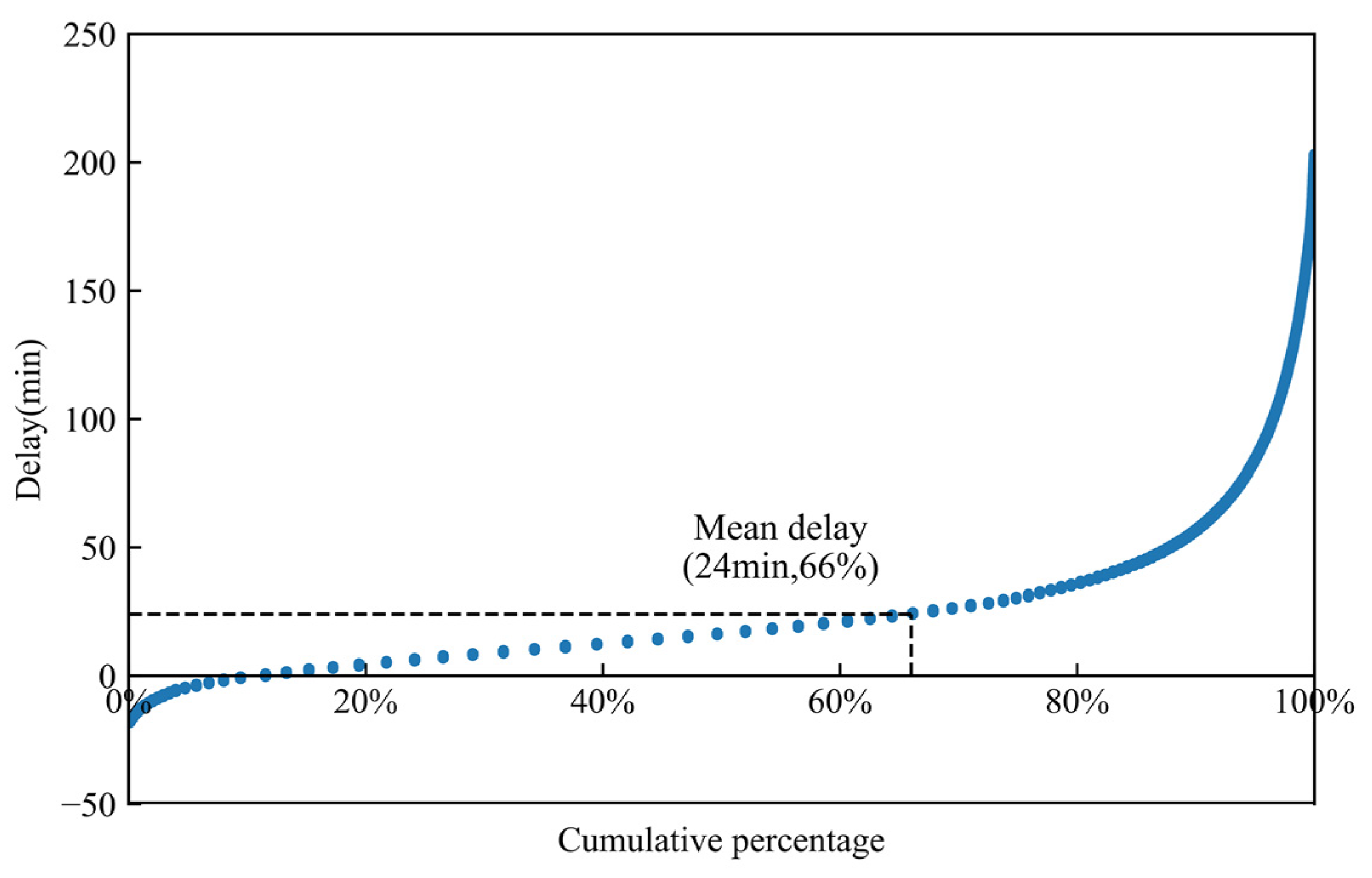
Our dataset comprised a total of 640,555 flight records, including all arrival and departure flights. Key fields included flight number, airline, aircraft register number, take-off and landing time, delays, etc. Delays were positive or negative, with a negative number indicating that the actual time was earlier than the scheduled time, which can have a significant impact on actual operations and is therefore within the scope of this paper. Figure 2 depicts the distribution of flight delays after removing the top and bottom 1% of delay values.
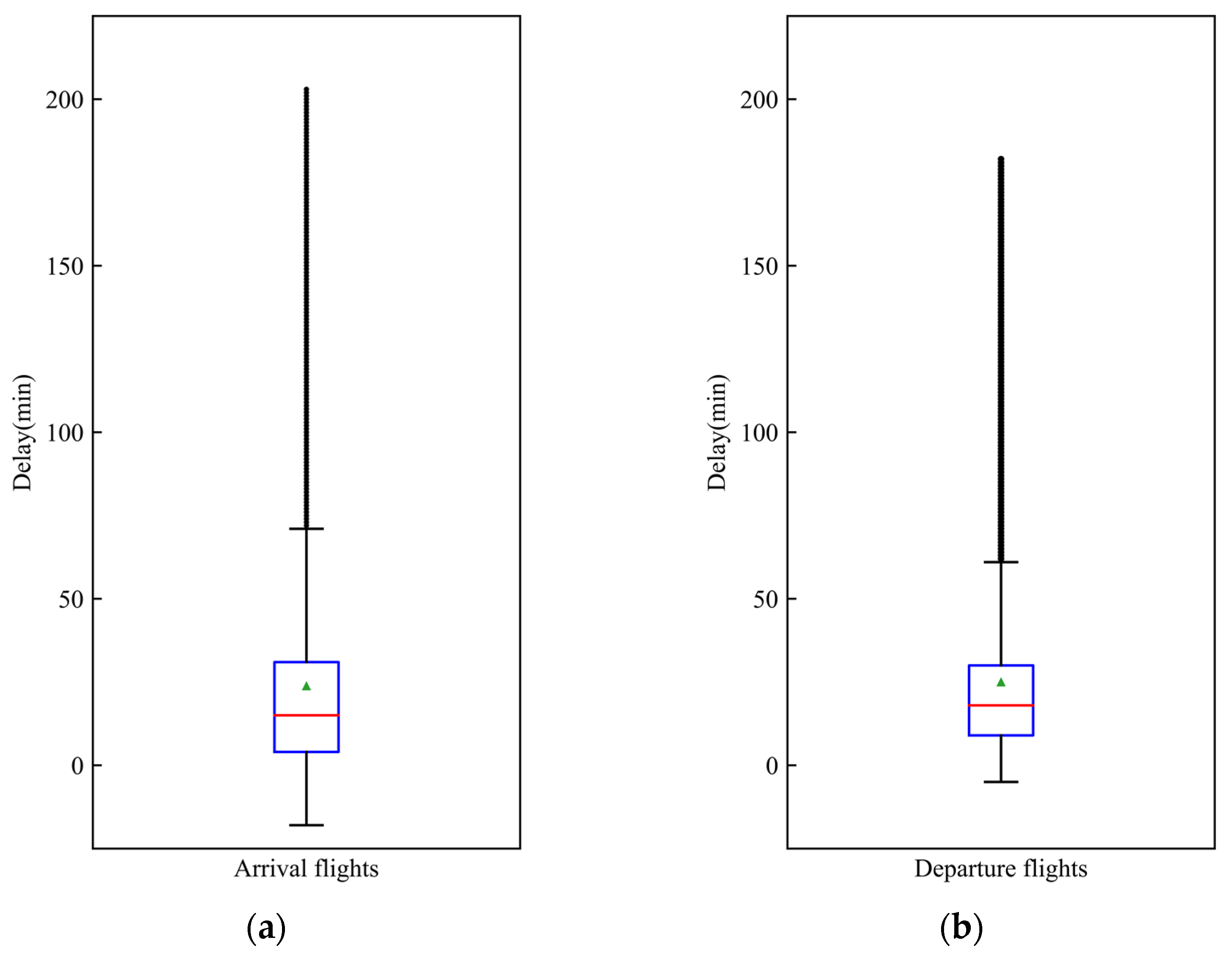
Note that approximately 10% of flights had negative delay values, among which nearly 80% were arrival flights. Figure 3 shows that the arrival flight delays had higher quartile values and outliers than departure flights, and arrival flights had more negative delay values. Airlines sometimes overstate flight times to create a buffer for unpredictable events, resulting in negative delay values [20]. While this overstatement may offset delays caused by other factors, it can affect the accuracy of predictions. Thus, to avoid such errors, we focused on departure flights.
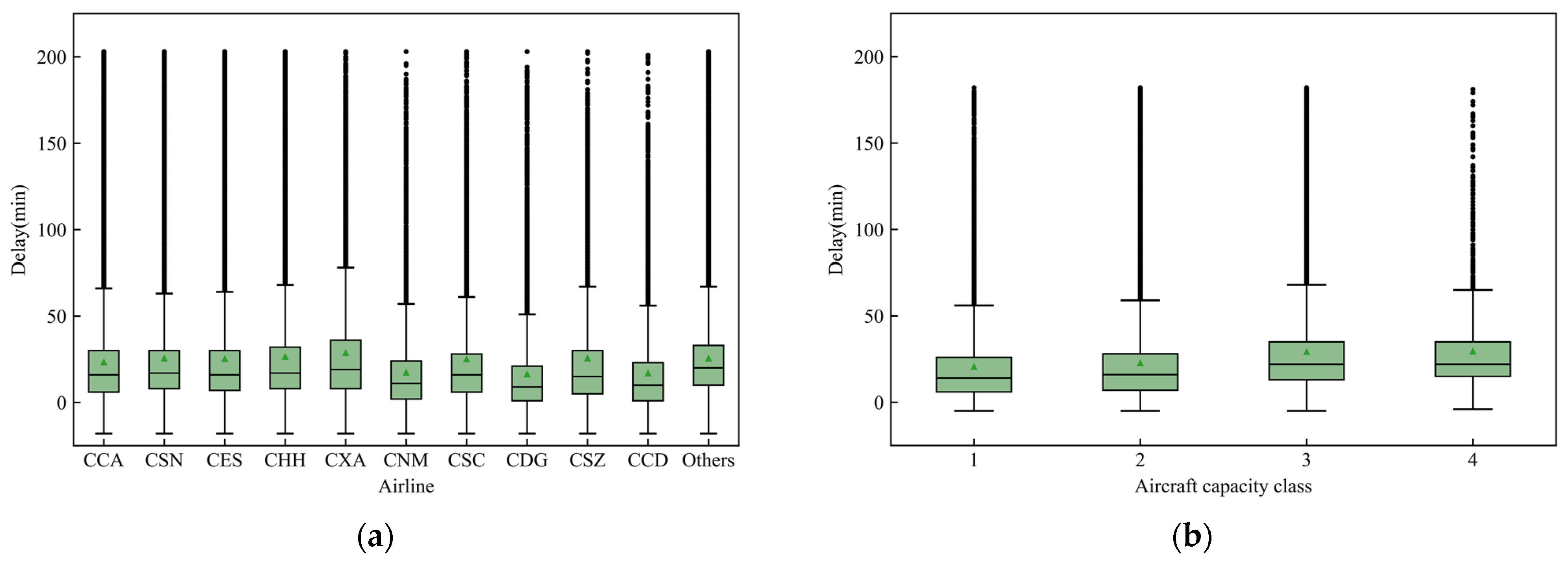
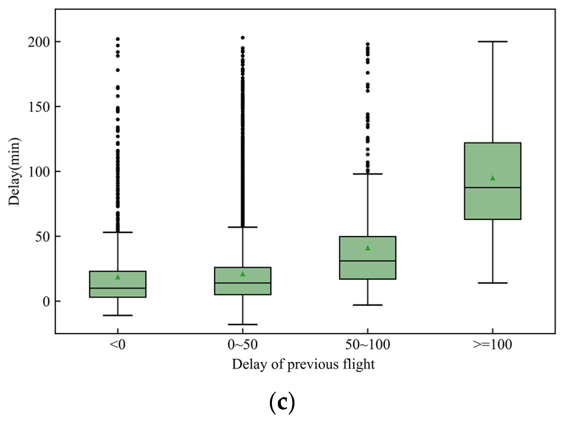
In Figure 4a, the abscissas for the airline are airline codes assigned by the International Civil Aviation Organization (ICAO). There were significant differences in the distribution of flight delays between airlines. The figure shows only the distribution of delays for the top 10 airlines separately in terms of flight volume. There were four aircraft capacity classes in our dataset, and class 3 had the highest average delay, see Figure 4b. As shown in Figure 4c, when the delay of previous flight was greater than 50 min, the delay of current flight also increased, indicating that the current flight was likely to be affected by the delay of the previous flight.
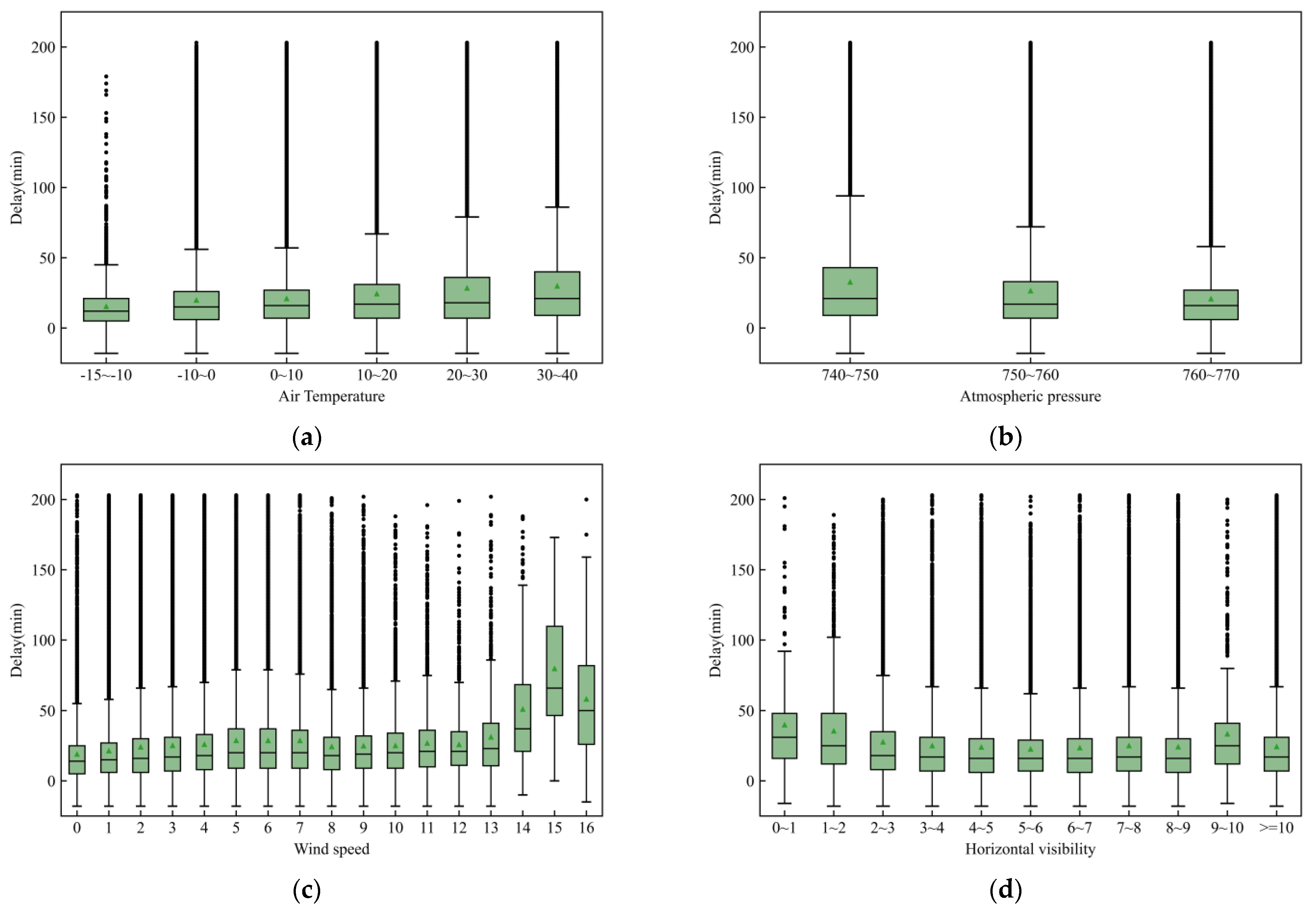
As Figure 5a shows, when the air temperature was between −10 and 20 °C, the distribution of delay was more stable and concentrated. The average delay increased when the temperature was between 20 and 40 °C. Although low temperatures may cause flight delays due to icing of the runway, there were no extreme delay values in this dataset, having possibly been removed as outliers during data preprocessing. As indicated in Figure 5b, the average delay was higher when the atmospheric pressure was lower, which may be due to the relationship between atmospheric pressure and weather. For example, atmospheric pressure is lower during bad weather, such as on rainy days compared with sunny days. When horizontal visibility is low, such as in severe haze, flights are delayed for safety reasons. Similarly, high wind speeds are not conducive to safe take-off and landing, resulting in increased average delays.
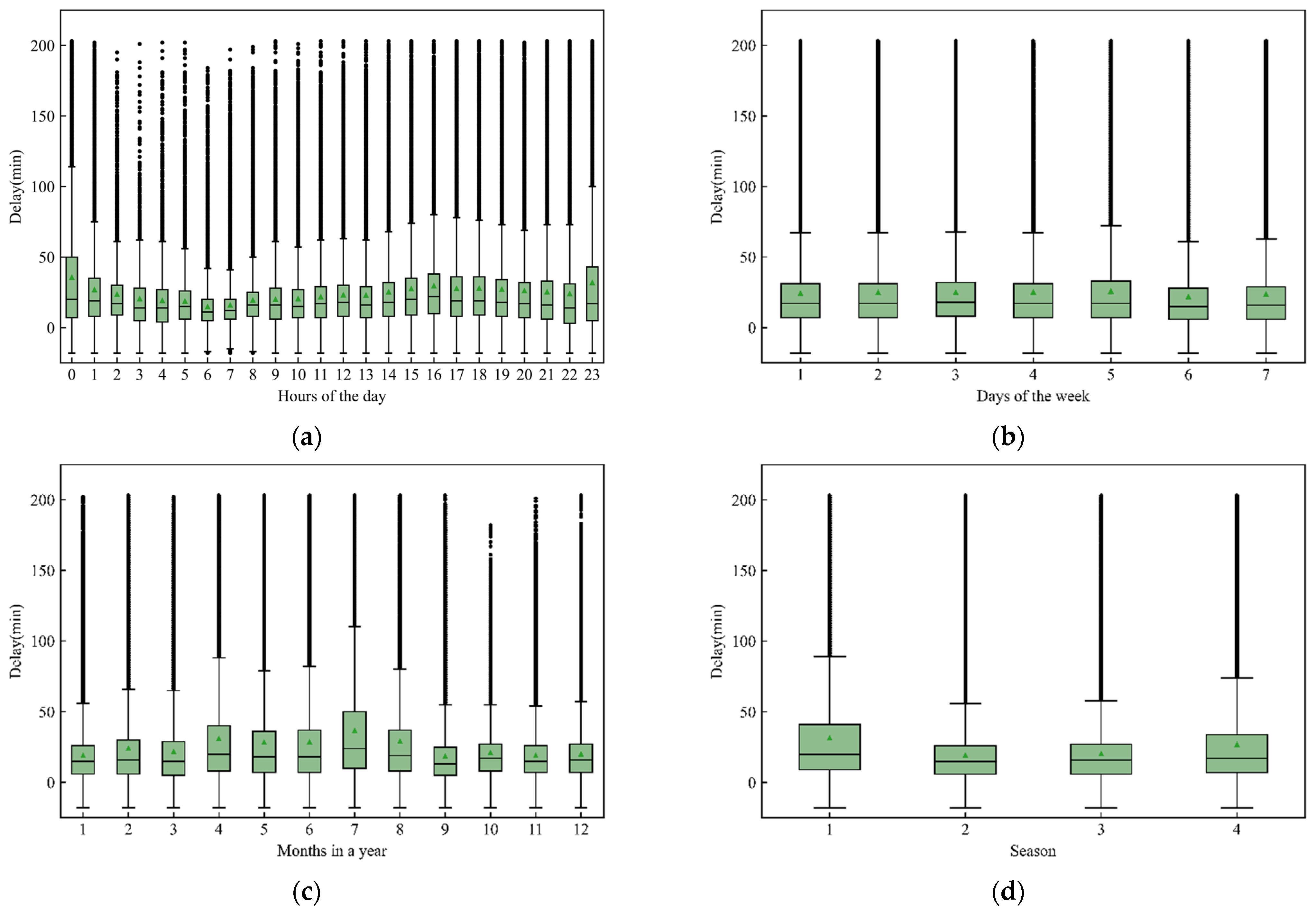
In Figure 6a, 0 indicates 00:00–00:59 and 23 is 23:00–23:59. In Figure 6b, the digits 1–7 indicate Monday to Sunday, respectively. In Figure 6c, 1–12 refer to January to December, respectively. In Figure 6d, seasons 1, 2, 3, and 4 respectively denote June to August, September to November, December to February, and March to May. The statistical characteristics of periodic data varied only slightly in most cases. However, some periods had higher average delays. For example, June to August is the peak tourist season with frequent changes of weather, so the average delay was higher than in other seasons.
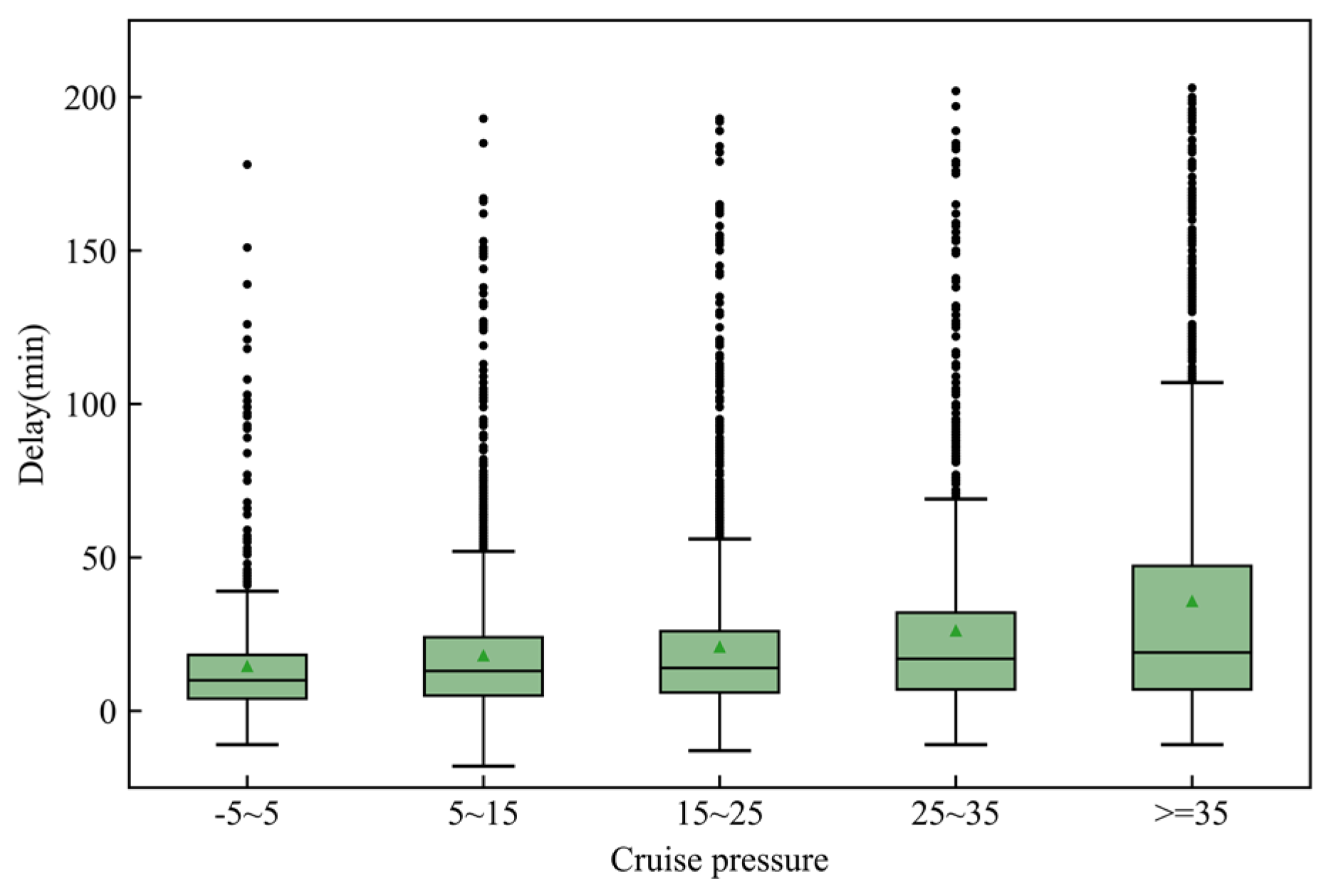
Figure 7 and Figure 8 show the departure pressure and cruise pressure, respectively, for flights from PEK to HGH. Departure pressure refers to the number of scheduled flights and the actual number of flights within a certain period. As shown in Figure 7a, the average delay grew slowly as the number of scheduled flights increased. The same situation occurred when the number of actual flights was less than 80. However, when the number of actual flights was greater than 80, the average delay showed a significant decrease, which presents an anomaly. This may be because the sample size for this section was small and not representative. Figure 8 indicates that cruise pressure and average delay were positively correlated.

4.2. Data Preprocessing

Data cleaning and handling were very important when building the model, so flight records were deleted if they contained unfillable missing values for necessary attributes such as scheduled departure time. For fillable data, such as weather variables, if the value was missing at hour t , the value at its previous hour t 1 was used in place of the missing value. In addition, the top and bottom 1% of delays were also eliminated as outliers. The cleaned data was randomly divided into two subsets: 80% of the data were used for training and the rest were used for testing. In this study, we predicted flight delays 2 h before the scheduled time, i.e., τ = 2 . A summary of the handling mode for explanatory variables is listed in Table 4. Some discrete variables, such as airline, were treated as 0–1 dummy variables, while other discrete variables, such as hour of the day and day of the week, were handled by sine–cosine functions in order to preserve periodicity. In addition, variables such as delay of previous flights were calculated. To improve the accuracy of the model and enhance convergence speed, the continuous data were normalized:
x * = x μ σ
where x * is a normalized variable; x , μ , and σ are original variable, average value, and standard deviation, respectively.
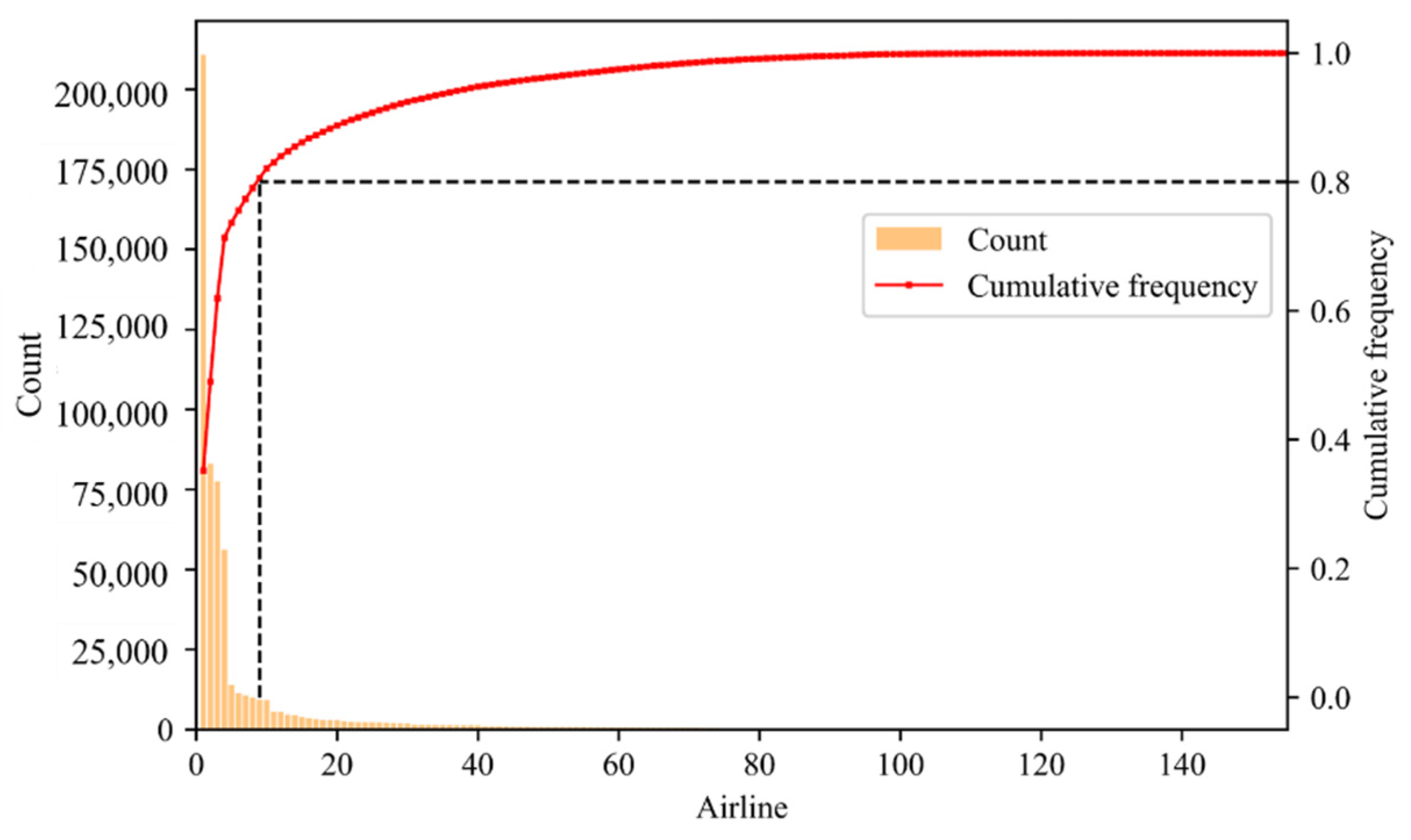
In our study, the airline variable was handled by one-hot encoding. However, there were 155 airlines in total, and direct use of one-hot encoding would increase the dimensions of the dataset and affect the training speed. Therefore, we applied the Pareto principle to the airline data [30]. As shown in Figure 9, the top 10 airlines accounted for 82.13% of all flights in total.
As shown in Table 5, using one-hot encoding an airline would be represented by one row and 155 columns of data, while using Pareto encoding, only one row and 11 columns of data were needed.
In order to improve the efficiency of the calculation without affecting the results, the flight data for the routes with the five highest similarity coefficients were utilized to calculate the cruise pressure [19]. Table 6 lists the top five air routes for PEK to HGH with the highest similarity coefficients.

4.3. Variable Selection

Efficient models of machine learning rely on a strong correlation between the input variables and the target values. The processed dataset contained 18 factors related to flight delays. While a large dataset may be beneficial for prediction, too many uncorrelated factors may lead to overfitting or underfitting.
Feature selection methods are mainly divided into three categories: filter methods, wrapper methods, and embedded methods [31]. Filtering methods have been widely used due to their fast computation and model-independent advantages. We used two filter methods before running the prediction model, namely, mutual information and correlation coefficient.
As a result, five factors were removed because of their low performances in both the mutual information and correlation coefficient methods. The removed factors were whether the airport was used as a base, day of the week, whether it was a holiday, wind direction, and horizontal visibility. Ultimately, the remaining 13 factors were used as inputs in the model.

4.4. Base Learners

The ensemble methods described in the “Methodology” section, including bagging, boosting, and stacking methods, were employed to predict flight delay. In addition to the RF algorithm and the AdaBoost algorithm, other well-known methods were also selected as candidates for base learners in the stacking model, and are briefly introduced here:
  • Linear regression (LR): LR is a classical regression method that uses a linear model to fit the relationship between features and target values.
  • K-nearest neighbor (KNN): KNN uses the average of the closest K samples of a sample to represent its value. Manhattan and Euclidean distances are usually used.
  • Support vector regression (SVR): SVR involves the application of a support vector machine (SVM) for regression problems. It works by locating a hyperplane so that the distance from the hyperplane to the farthest sample point is minimized.
  • Light gradient boosting machine (LGBM): LGBM is a framework for implementing the gradient boosting decision tree (GBDT) algorithm, which supports efficient parallel training and has faster training speed, lower memory consumption, and better accuracy.

5. Results and Discussion

In this section, we present the delay prediction results for flights from PEK to HGH, and discuss some of the factors associated with delays.

5.1. Predicting Results

To enhance the performance of the model, the parameters of each algorithm were determined by the grid-search method. If the result of a certain algorithm was not unique, we ran it ten times to obtain the average of the performance metrics. To avoid overfitting, we used five-fold cross-validation on the original training set. All algorithms were implemented using Python 3.9 on a computer with an octa-core 3.2-GHz CPU and 16-GB random-access memory. From the six regression models, the four models with optimal performance indicators were selected as base learners. After testing, we chose SVR as a meta-learner.
Table 7 shows the prediction performance based on the test dataset. The results confirm that stacking method outperformed the other five baseline methods and achieved high-performance predictions based on high-dimensional data.
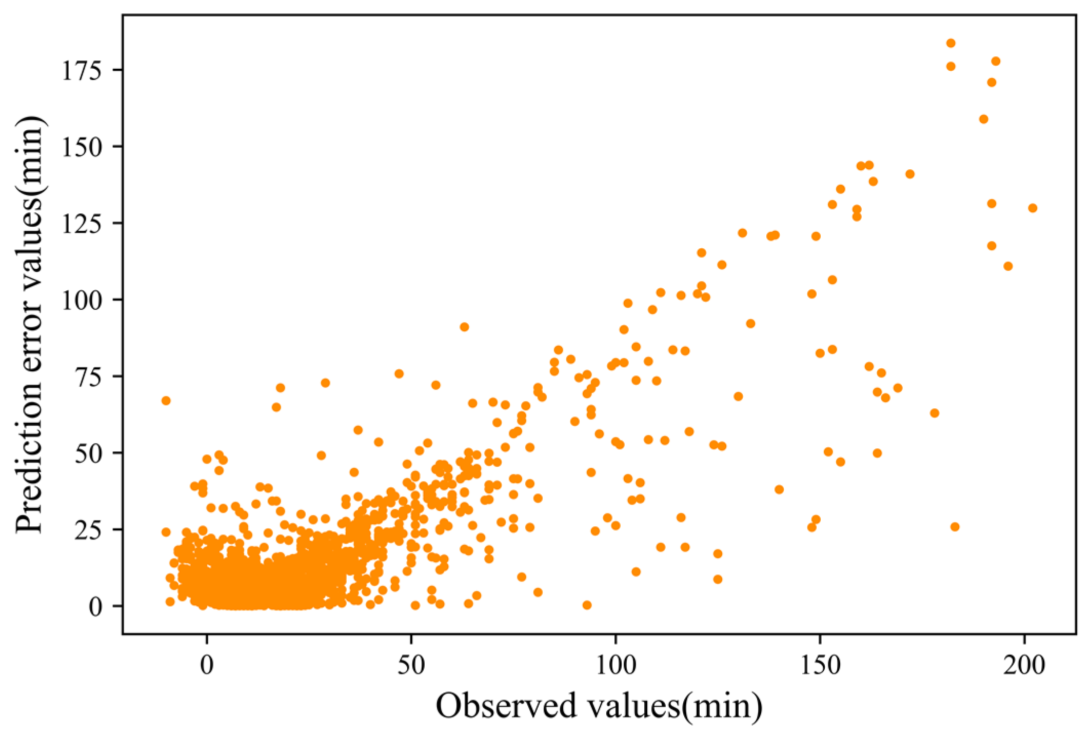
Figure 10 shows the distribution of error values for the predictions with the observed values. The error values increased with the growth of the observed values. When the observed values were larger than 60 min, the prediction error started to increase, implying a decrease in accuracy. It was found that 95.7% of the predicted values were within 35 min deviation from the observed values, implying an acceptable prediction performance.
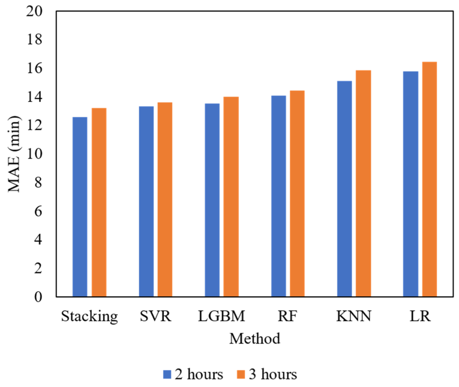
Figure 11 shows the results of predictions at τ = 2 and τ = 3 , that is, predicted 2 h and 3 h ahead. When τ = 3 , the prediction error increased, but stacking method continued to outperform the other methods.
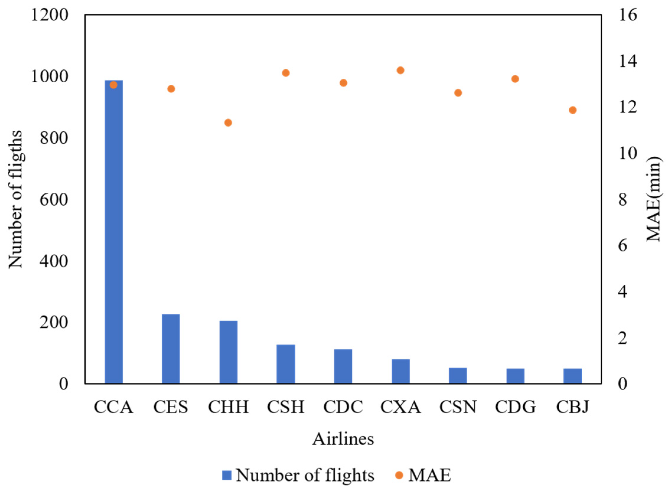
The predictions for different airlines were stable in view of the small gap in MAE values of the nine airlines. As shown in Figure 12, there was no strong correlation between MAE and the number of flights, indicating that the model was robust for different airlines regardless of their numbers of flight records.
Four scenarios with different explanatory variables were set to validate the novel variables proposed in this paper. As Table 8 shows, S0 is the initial scenario, including flight attributes, weather, and periodic data. S1 and S2 are the scenarios after the addition of arrival pressure and cruise pressure, respectively. S3 is the set of all explanatory variables. The results show that the arrival pressure and cruise pressure were very important for improving model performance.
We encoded the periodic data with one-hot encoding and sine–cosine functions, and input the data into the model for prediction. The performance comparison of different encoding methods of periodic data is shown in Table 9. It was found that the prediction model achieved better performance with sine–cosine function encoding than one-hot encoding of periodic data. This method was better able to interpret the periodic explanatory variables. The method not only improved performance, but was also interpretable.

5.2. Delay of Previous Flight

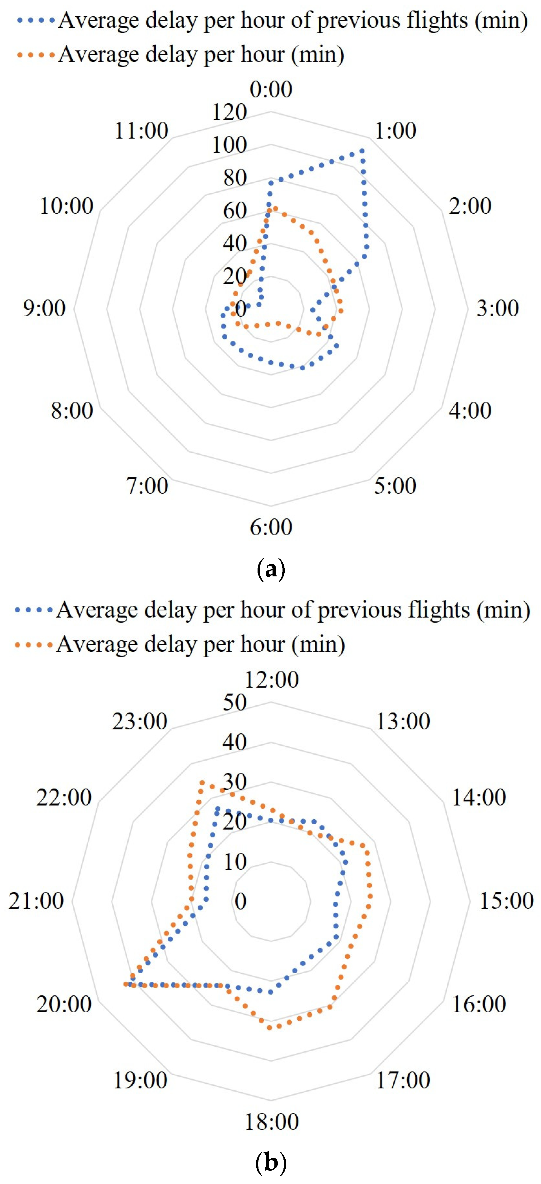
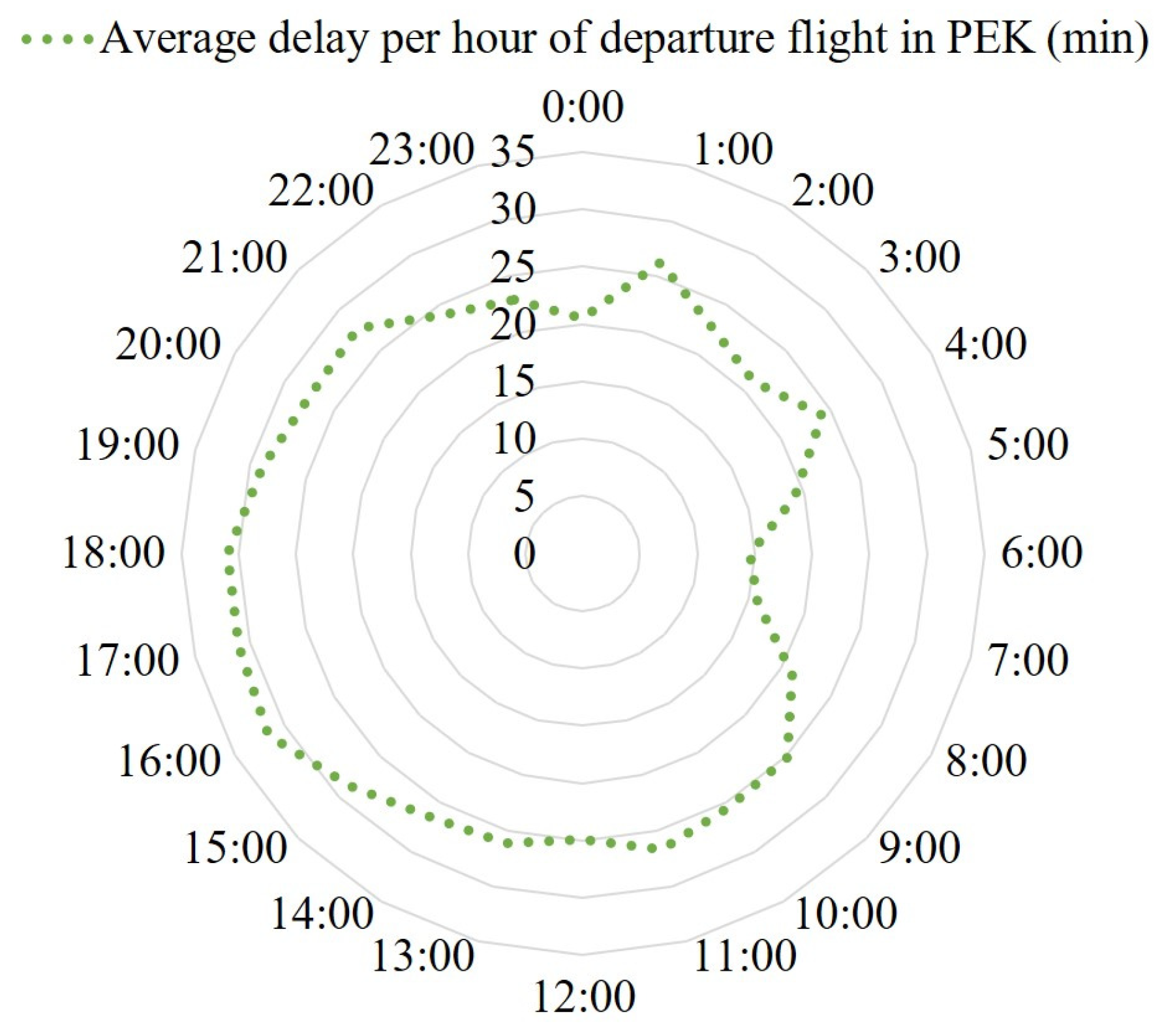
Delay of the previous flight was a key influential factor on flight delays. In this subsection, we focus on the relationship between delay of the previous flight and delay propagation. Figure 13 depicts flight delay and delay of previous flight (the same flight register number) per hour for two different time frames (Figure 13a: 00:00–12:00, Figure 13b: 12:00–24:00), for PEK to HGH. Figure 13b shows a correlation between the flight delay and the delay of the previous flight during the period 12:00–24:00. After calculation, the Pearson correlation coefficient was 0.78, confirming a strong correlation. Figure 14 shows the average delay per hour of departure flights at PEK. Apparently, delays were higher in the afternoon and evening (12:00–22:00).
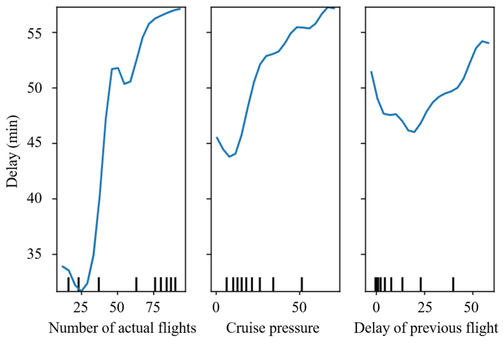
The marginal effect of features on the prediction results of the model was captured by partial dependence plot (PDP). Figure 15 shows the PDP of delay of previous flight, number of actual flights, and cruise pressure. The scale on the horizontal axis is the location of the concentration of values. Considering delay propagation and absorption, it should be noted that the interval between the previous flight and the current flight is included in Equation (1). In other words, the greater the interval between two flights, the smaller the delay of the previous flight. Figure 15 shows that when the delay of the previous flight was less than 22, the delay of the current flight decreased. This may be due to the long interval between the two flights, where the delay of the previous flight was largely absorbed and was not the main factor causing the current flight delay. However, when the delay of the previous flight increased from 22 to 50, the delay of the current flight increased because the interval between the two flights was too short for the delay to be absorbed.
This suggests that airlines should increase the time interval between two flights using the same aircraft, but only for smaller airlines. From the airport’s point of view, the flight turnaround time should be shortened as much as possible to reduce the impact of the delay of the previous flight on the subsequent flight. Moreover, scheduling flights in the morning is a good option, although the balance flight schedules must also be considered.

5.3. Departure Pressure

As shown in Figure 15, the marginal effect of departure pressure on delay tended to increase when the number of actual flights was greater than 25. The departure pressure defined in this paper can also reflect the congestion level of the airport to some extent.

5.4. Cruise Pressure

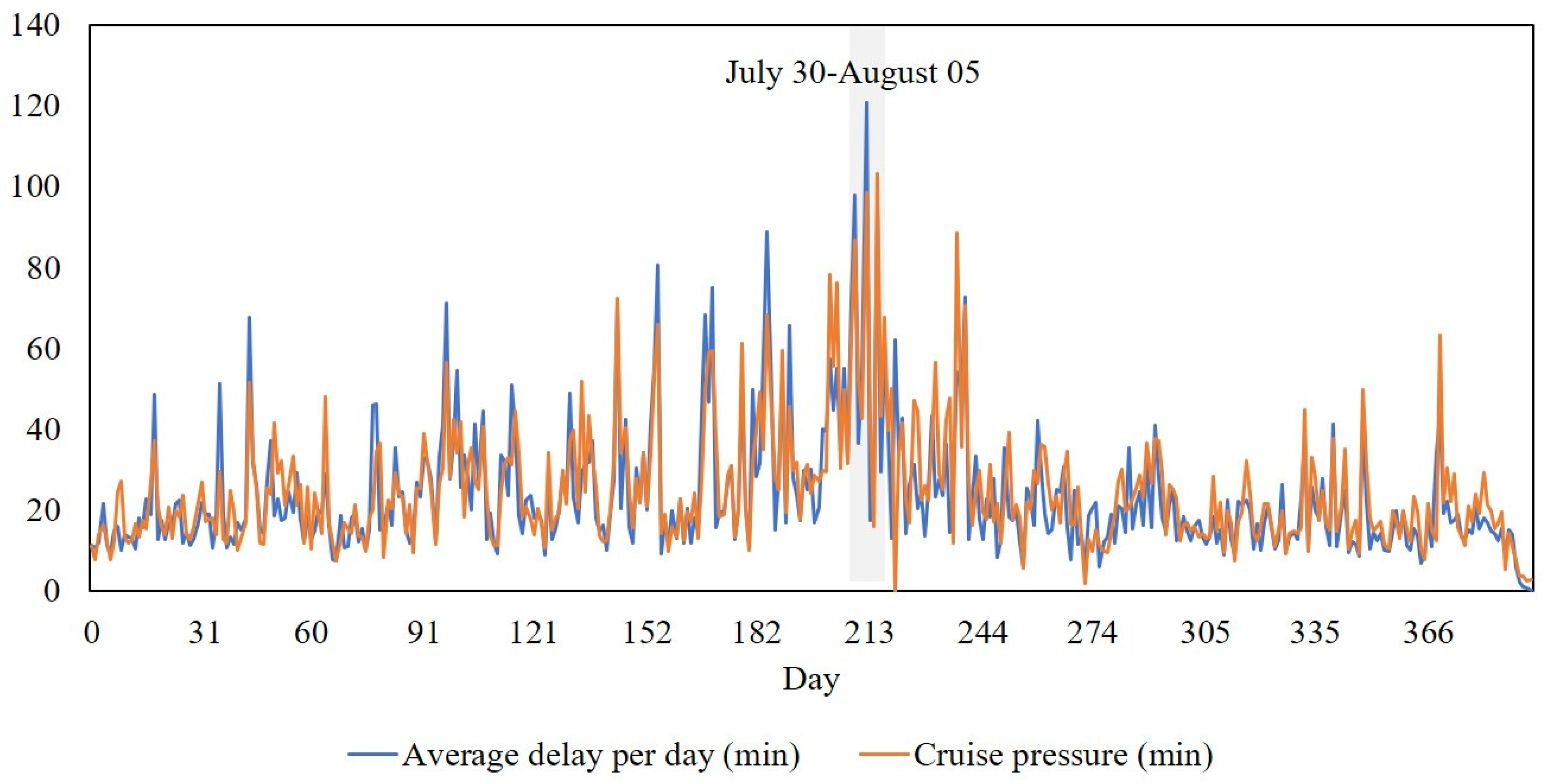
In Section 3.2.5, cruise pressure was proposed to represent the condition of the air route. Figure 16 depicts the average cruise pressure and the average delay per day of PEK–HGH flights from 1 January 2019 to 31 January 2020. It can be observed that flight delays and cruise pressure were consistent in most cases. The Pearson correlation coefficient was 0.81, which confirms a strong positive correlation. Additionally, the cruise pressure during 30 July and 5 August was significantly different from the other time frames, while the average delay was higher than in the other time frames. Checking the historical weather data, we interestingly found that there was rainfall, hail, and other severe weather in Beijing at that time. The observation shows that the method used in this paper to represent air-route condition is valid and can be used to predict delay.
Figure 15 shows that the marginal effect of cruise pressure on delay tended to increase. There was a slight drop in delay before cruise pressure was 0 compared with the first concentrated value. This means that cruise pressure was not the main factor affecting flight delays. As cruise pressure increased, it indicated that the air route was more congested, resulting in increased delays.

6. Conclusions

With the rapid development of the civil aviation industry and growing demand for air traffic, flight delay is becoming more frequent. Flight delay not only affects passenger satisfaction, but can also cause huge economic losses. Therefore, development of a more advanced and accurate flight delay prediction method is an important research topic.
Ensemble methods are introduced in this paper, including bagging, boosting, and stacking methods. RF and AdaBoost were selected as the base learners for the stacking model, which are categorized as bagging and boosting methods, respectively. In addition, other common algorithms were selected as base learners. The results showed that the best prediction performance for the test dataset was obtained using the stacking method (MAE, 12.58; RMSE, 22.97). In the prediction results of the test dataset, 95.7% of the predicted values were within 35 min deviation from the observed values, implying an acceptable prediction performance.
This study focused on the use of macro and micro factors for predicting flight delay. We propose two novel explanatory variables from a microscopic perspective: departure pressure and cruise pressure. With the inclusion of these two variables, the MAE and RMSE for predictions using the stacking method were reduced by 20% and 12%, respectively. Moreover, cruise pressure can effectively characterize the congestion of the air route. To preserve the periodicity of data, values were converted to coordinates on a circle using the sine–cosine function. Compared with one-hot encoding, this type of encoding reduced MAE by 1.5% and RMSE by 1%. These were small improvements, but beneficial in predicting flight delay and deserving of further study. To reduce the dimensionality of data and speed up the model, airlines were coded using the Pareto encoding method.
This study has many limitations. Flight delays are not only related to the departure airport, but information from the arrival airport also has a potential impact on flight delays. Due to the lack of data, information from the arrival airport was not used in these predictions. Therefore, information from arrival and departure airports should be utilized to enhance the performance of the model. During the calculation of cruise pressure, flights on five similar routes were considered; in future, more national and international routes can be considered. Additionally, this paper does not consider the effect of interactions between airports on the propagation of delays, which is a direction for future research.

Author Contributions

Conceptualization, X.W., Z.W., L.W. and Y.T.; methodology, Z.W.; software, X.W.; validation, X.W., L.W. and Y.T.; formal analysis, X.W.; investigation, X.W.; resources, Y.T.; data curation, L.W.; writing—original draft preparation, X.W.; writing—review and editing, Z.W.; visualization, X.W.; supervision, Z.W., L.W. and Y.T.; project administration, Y.T.; funding acquisition, Y.T. All authors have read and agreed to the published version of the manuscript.

Funding

This research was funded by the National Natural Science Foundation Project of China (U1933119).

Institutional Review Board Statement

Not applicable.

Informed Consent Statement

Not applicable.

Data Availability Statement

Not applicable.

Conflicts of Interest

The authors declare no conflict of interest.

Nomenclature

i flight t i s scheduled time of flight i
F A flight attributes t i p a real time of the previous of flight i
Wweather n s number of scheduled flights
P D periodic data n a number of actual flights
A P arrival pressure s c j similarity degree of air routes between specific flights
C P cruise pressure t c j time coefficient
τ advance prediction interval d j delay of flight j

References

  1. Civil Aviation Administration of China. 2019 Civil Aviation Industry Development Statistic Bulletin; Civil Aviation Administration of China: Beijing, China, 2019; p. 14.
  2. United States Department of Transportation. Understanding the Reporting of Causes of Flight Delays and Cancellations [EB/OL]. Available online: http://www.bts.dot.gov/topics/airlines-and-airports/understanding-reporting-causes-flight-delays-and-cancellations (accessed on 6 September 2022).
  3. Ekici, F.; Orhan, G.; Gümüş, Ö.; Bahce, A.B. A Policy on the Externality Problem and Solution Suggestions in Air Transportation: The Environment and Sustainability. Energy 2022, 258, 124827. [Google Scholar] [CrossRef]
  4. Ekici, S.; Şöhret, Y.; Gürbüz, H. Influence of COVID-19 on Air Pollution Caused by Commercial Flights in Turkey. Energy Sources Part A Recov. Util. Environ. Eff. 2021, 43, 1–13. [Google Scholar] [CrossRef]
  5. Hsiao, C.; Hansen, M. Econometric analysis of US airline flight delays with time-of-day effects. Transp. Res. Rec. 2006, 1951, 104–112. [Google Scholar] [CrossRef]
  6. Tu, Y.; Ball, M.O.; Jank, W.S. Estimating flight departure delay distributions—A statistical approach with long-term trend and short-term pattern. J. Am. Stat. Assoc. 2008, 103, 112–125. [Google Scholar] [CrossRef]
  7. Rodríguez-Sanz, Á. Assessment of Airport Arrival Congestion and Delay: Prediction and Reliability. Transp. Res. Part C Emerg. Technol. 2019, 98, 255–283. [Google Scholar] [CrossRef]
  8. Rebollo, J.J.; Balakrishnan, H. Characterization and Prediction of Air Traffic Delays. Transp. Res. Part C Emerg. Technol. 2014, 44, 231–241. [Google Scholar] [CrossRef]
  9. Esmaeilzadeh, E.; Mokhtarimousavi, S. Machine Learning Approach for Flight Departure Delay Prediction and Analysis. Transp. Res. Rec. J. Transp. Res. Board 2020, 2674, 145–159. [Google Scholar] [CrossRef]
  10. Kim, Y.J.; Choi, S.; Briceno, S.; Mavris, D. A Deep Learning Approach to Flight Delay Prediction. In Proceedings of the 2016 IEEE/AIAA 35th Digital Avionics Systems Conference (DASC), Sacramento, CA, USA, 25–29 September 2016; pp. 1–11. [Google Scholar]
  11. Li, L.; Chen, X.; Zhang, L. Multimodel Ensemble for Freeway Traffic State Estimations. IEEE Trans. Intell. Transp. Syst. 2014, 15, 1323–1336. [Google Scholar] [CrossRef]
  12. Zhang, Y.; Haghani, A. A Gradient Boosting Method to Improve Travel Time Prediction. Transp. Res. Part C Emerg. Technol. 2015, 58, 308–324. [Google Scholar] [CrossRef]
  13. Wang, Z. Automated Data-Driven Prediction on Aircraft Estimated Time of Arrival. J. Air Transp. Manag. 2020, 88, 101840. [Google Scholar] [CrossRef]
  14. Du, W.B.; Zhang, M.Y.; Zhang, Y.; Cao, X.B.; Zhang, J. Delay Causality Network in Air Transport Systems. Transp. Res. Part E Logist. Transp. Rev. 2018, 118, 466–476. [Google Scholar] [CrossRef]
  15. Choi, S.; Kim, Y.J.; Briceno, S.; Mavris, D. Prediction of Weather-Induced Airline Delays Based on Machine Learning Algorithms. In Proceedings of the 2016 IEEE/AIAA 35th Digital Avionics Systems Conference (DASC), Sacramento, CA, USA, 25–29 September 2016; pp. 1–6. [Google Scholar]
  16. Gui, G.; Liu, F.; Sun, J.; Yang, J.; Zhou, Z.; Zhao, D. Flight Delay Prediction Based on Aviation Big Data and Machine Learning. IEEE Trans. Veh. Technol. 2020, 69, 140–150. [Google Scholar] [CrossRef]
  17. Stefanovič, P.; Štrimaitis, R.; Kurasova, O. Prediction of Flight Time Deviation for Lithuanian Airports Using Supervised Machine Learning Model. Comput. Intell. Neurosci. 2020, 2020, 8878681. [Google Scholar] [CrossRef] [PubMed]
  18. Ye, B.; Liu, B.; Tian, Y.; Wan, L. A Methodology for Predicting Aggregate Flight Departure Delays in Airports Based on Supervised Learning. Sustainability 2020, 12, 2749. [Google Scholar] [CrossRef] [Green Version]
  19. Guo, Z.; Yu, B.; Hao, M.; Wang, W.; Jiang, Y.; Zong, F. A Novel Hybrid Method for Flight Departure Delay Prediction Using Random Forest Regression and Maximal Information Coefficient. Aerosp. Sci. Technol. 2021, 116, 106822. [Google Scholar] [CrossRef]
  20. Yu, B.; Guo, Z.; Asian, S.; Wang, H.; Chen, G. Flight Delay Prediction for Commercial Air Transport: A Deep Learning Approach. Transp. Res. Part E Logist. Transp. Rev. 2019, 125, 203–221. [Google Scholar] [CrossRef]
  21. Zeng, W.; Li, J.; Quan, Z.; Lu, X. A Deep Graph-Embedded LSTM Neural Network Approach for Airport Delay Prediction. J. Adv. Transp. 2021, 2021, 6638130. [Google Scholar] [CrossRef]
  22. Bao, J.; Yang, Z.; Zeng, W. Graph to Sequence Learning with Attention Mechanism for Network-Wide Multi-Step-Ahead Flight Delay Prediction. Transp. Res. Part C Emerg. Technol. 2021, 130, 103323. [Google Scholar] [CrossRef]
  23. Cai, K.; Li, Y.; Fang, Y.-P.; Zhu, Y. A Deep Learning Approach for Flight Delay Prediction Through Time-Evolving Graphs. IEEE Trans. Intell. Transp. Syst. 2021, 23, 11397–11407. [Google Scholar] [CrossRef]
  24. Ren, Y.; Zhang, L.; Suganthan, P.N. Ensemble Classification and Regression-Recent Developments, Applications and Future Directions [Review Article]. IEEE Comput. Intell. Mag. 2016, 11, 41–53. [Google Scholar] [CrossRef]
  25. Zhang, J.; Peng, Z.; Yang, C.; Wang, B. Data-driven Flight Time Prediction for Arrival Aircraft within the Terminal Area. IET Intell. Transp. Syst. 2022, 16, 263–275. [Google Scholar] [CrossRef]
  26. Gui, X.; Zhang, J.; Peng, Z.; Yang, C. Data-Driven Method for the Prediction of Estimated Time of Arrival. Transp. Res. Rec. J. Transp. Res. Board 2021, 2675, 1291–1305. [Google Scholar] [CrossRef]
  27. Top 6 Errors Novice Machine Learning Engineers Make. Available online: https://www.kdnuggets.com/2017/10/top-errors-novice-machine-learning-engineers.html (accessed on 6 September 2022).
  28. Feature Engineering—Handling Cyclical Features. Available online: http://blog.davidkaleko.com/feature-engineering-cyclical-features.html (accessed on 6 September 2022).
  29. Gürbüz, H.; Şöhret, Y.; Ekici, S. Evaluating Effects of the Covid-19 Pandemic Period on Energy Consumption and Enviro-Economic Indicators of Turkish Road Transportation. Energy Sources Part A Recov. Util. Environ. Eff. 2021, 43, 1–13. [Google Scholar] [CrossRef]
  30. Wang, F.; Bi, J.; Xie, D.; Zhao, X. Flight Delay Forecasting and Analysis of Direct and Indirect Factors. IET Intell. Transp. Syst. 2022, 16, 890–907. [Google Scholar] [CrossRef]
  31. Pudil, P.; Hovovicova, J. Novel Methods for Subset Selection with Respect to Problem Knowledge. IEEE Intell. Syst. 1998, 13, 66–74. [Google Scholar] [CrossRef]
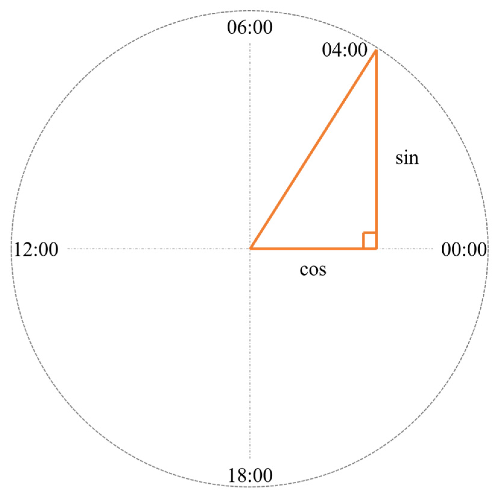
Figure 1. The circle of hours of the day.
Applsci 12 10621 g001
Figure 2. Cumulative distribution of flight delays.
Applsci 12 10621 g002
Figure 3. Quartile diagram of arrival and departure flights; (a) arrival flights, (b) departure flights.
Applsci 12 10621 g003
Figure 4. Factors influencing flight attributes: (a) airline, (b) aircraft capacity class, (c) delay of previous flight.
Applsci 12 10621 g004aApplsci 12 10621 g004b
Figure 5. Influencing factors relating to weather: (a) air temperature, (b) atmospheric pressure, (c) wind speed, (d) horizontal visibility.
Applsci 12 10621 g005
Figure 6. Temporal variation in flight delays: (a) hour of the day, (b) day of the week, (c) month of the year, (d) season.
Applsci 12 10621 g006
Figure 7. Departure pressure of flights from PEK to HGH: (a) number of scheduled flights, (b) number of actual flights.
Applsci 12 10621 g007
Figure 8. Cruise pressure of flights from PEK to HGH.
Applsci 12 10621 g008
Figure 9. Bar chart and cumulative frequency curve of flight data grouped by airline.
Applsci 12 10621 g009
Figure 10. Distribution of the prediction error values and the observed values.
Applsci 12 10621 g010
Figure 11. MAE comparison for τ = 2 and τ = 3 .
Applsci 12 10621 g011
Figure 12. MAE and number of flights per airline.
Applsci 12 10621 g012
Figure 13. Average delay per hour of flights from PEK to HGH and their previous flights; (a) 00:00–12:00, (b) 12:00–24:00.
Applsci 12 10621 g013
Figure 14. Average delay per hour of departure flights at PEK.
Applsci 12 10621 g014
Figure 15. Partial dependence plots.
Applsci 12 10621 g015
Figure 16. Cruise pressure of PEK–HGH flights (1 January 2019–31 January 2020).
Applsci 12 10621 g016
Table 1. Summary of previous studies.
ReferenceMethodologyConsidered Factors
Tu et al. (2008) [6]Statistical modeling methodsSeasonal trends, daily propagation, and random residuals
Choi et al. (2016) [15]Traditional MLQuarter of year, month, day of month, day of week, departure and arrival schedule in local time, and weather
Rebollo et al. (2014) [8]Traditional MLTemporal variables, delay state, type of delay, previous day’s type, delay at influential airports, and OD pairs
Gui et al. (2020) [16]Traditional ML and DLWeather, day of month, month, day of week, and season
Stefanovič et al. (2020) [17]Traditional MLDeparture airport, scheduled time of departure, destination, scheduled time of arrival, date of the flight, ICAO identity number, and flight number
Ye et al. (2020) [18]Traditional MLTime characteristics, flight plan characteristics, delay characteristics, and local weather characteristics
Guo et al. (2021) [19]Traditional MLAirline size, actual aircraft capacity, scheduled turnaround time, minimum turnaround time, origin or pass-by flight, delay of the previous flight, crowdedness of the airport in terms of number of flights and passengers
Yu et al. (2019) [20]DLAir-route situation, delay of previous flight, airline properties, number of passengers, aircraft capacity, boarding options, air traffic control, and crowdedness of airport
Zeng et al. (2021) [21]DLSpherical distance between airports, airports’ history of hourly average delay
Bao et al. (2021) [22]DLAirports’ history of hourly average delay, weather
Cai et al. (2021) [23]DLAirports’ history of hourly average delay
Table 2. Aircraft capacity class table.
Number of SeatsRepresentative Aircraft TypeGrade Number
Less than 60 seatsCRJ2, MA60, etc.0
61 to 150 seatsA319, B733, B734, B735, B736, B737, etc.1
151 to 250 seatsC919, A310, A320, A321, B738, B739, B788, etc.2
251 to 500 seatsA332, A333, A343, A346, A350, B742, etc.3
500 seats or moreA388, etc.4
Table 3. Reasons for abnormal flights in China in 2019.
Reasons for Abnormal FlightsPercentage of TotalCompared with Previous Year
Weather46.49%−0.96%
Airlines18.91%−2.22%
Air traffic control1.43%−0.88%
Others33.17%4.08%
Table 4. List of handling modes of explanatory variables.
Handling ModeExplanatory Variables
One-hot encoding methodAirline
0–1 modeledBase airport, holiday
CalculatedDelay of previous flight, arrival/departure pressure, cruise pressure, aircraft capacity
Sine–cosine functionsWind direction, hour of the day, day of the week, month of the year, season
No handlingAir temperature, atmospheric pressure, relative humidity, wind speed, horizontal visibility
Table 5. List of airlines encoding.
AirlinesProportionCFCountOne-HotPareto Principle
CCA35.18%35.18%210,821[1, 0, 0, …, 0][1, 0, 0, 0, 0, 0, 0, 0, 0, 0, 0]
CSN13.84%49.03%82,987[0, 1, 0, …, 0][0, 1, 0, 0, 0, 0, 0, 0, 0, 0, 0]
CES12.94%61.97%77,551[0, 0, 1, …, 0][0, 0, 1, 0, 0, 0, 0, 0, 0, 0, 0]
CHH9.37%71.34%56,157[0, 0, 0, …, 0][0, 0, 0, 1, 0, 0, 0, 0, 0, 0, 0]
CXA2.32%73.66%13,924[0, 0, 0, …, 0][0, 0, 0, 0, 1, 0, 0, 0, 0, 0, 0]
CNM1.90%75.57%11,435[0, 0, 0, …, 0][0, 0, 0, 0, 0, 1, 0, 0, 0, 0, 0]
CSC1.77%77.35%10,629[0, 0, 0, …, 0][0, 0, 0, 0, 0, 0, 1, 0, 0, 0, 0]
CDG1.68%79.03%10,076[0, 0, 0, …, 0][0, 0, 0, 0, 0, 0, 0, 1, 0, 0, 0]
CSZ1.56%80.59%9348[0, 0, 0, …, 0][0, 0, 0, 0, 0, 0, 0, 0, 1, 0, 0]
CCD1.55%82.13%9267[0, 0, 0, …, 0][0, 0, 0, 0, 0, 0, 0, 0, 0, 1, 0]
CBJ0.92%83.05%5519[0, 0, 0, …, 0][0, 0, 0, 0, 0, 0, 0, 0, 0, 0, 1]
[0, 0, 0, …, 0][0, 0, 0, 0, 0, 0, 0, 0, 0, 0, 1]
ANG0.0002%100%1[0, 0, 0, …, 1][0, 0, 0, 0, 0, 0, 0, 0, 0, 0, 1]
Table 6. Similarity coefficients of the top five air routes.
Air RouteSimilarity Coefficient
PEK–HGH1.00
PEK–YIW0.93
PEK–NKG0.82
PEK–CZX0.81
PEK–HYN0.75
Table 7. Predictive performance based on the test dataset.
StackingSVRLGBMRFAdaBoostKNNLR
MAE12.5813.313.5114.0514.5615.1115.78
RMSE22.9723.5923.8224.5024.6225.0126.16
Table 8. Performance comparison of different scenarios.
ScenarioExplanatory VariableMAERMSE
F A , W , P D A P C P
S0 15.6725.98
S1 14.8324.32
S2 13.2123.56
S312.5922.97
* F A , W , P D , A P and C P denote flight attributes, weather, periodic data, arrival pressure, and cruise pressure, respectively.
Table 9. Performance comparison of different encoding methods for periodic data.
Encoding MethodMAERMSE
One-hot encoding12.7823.18
Sine–cosine function12.5922.97
Publisher’s Note: MDPI stays neutral with regard to jurisdictional claims in published maps and institutional affiliations.