Abstract
Energy demand is rising sharply due to the technological development and progress of modern times. Neverthless, traditional thermal power generation has several diadvantages including its low energy usage and emitting a lot of polluting gases, resulting in the energy depletion crisis and the increasingly serious greenhouse effect. In response to environmental issues and energy depletion, the Combined Cooling, Heating and Power system (CCHP) combined with the power-generation system of renewable energy, which this work studied, has the advantages of high energy usage and low environmental pollution compared with traditional thermal power generation, and has been gradually promoted in recent years. This system needs to cooperate with the instability of renewable energy and the dispatch of the energy-saving system; the optimization of the system has been researched recently for this purpose. This study took Xikou village, Lieyu township, Kinmen county, Taiwan as the experimental region to solve the optimization problem of CCHP combined with renewable energy and aimed to optimize the multi-objective system including minimizing the operation cost, minimizing the carbon emissions, and maximizing the energy utilization rate. This study converted the original multi-objective optimization problem into a single-objective optimization problem by using the Technique for Order Preference by Similarity to and Ideal Solution (TOPSIS) approach. In addition, a hybrid of the simplified swarm optimization (SSO) and differential evolution (DE) algorithm, called SSO-DE, was proposed in this research to solve the studied problem. SSO-DE is based on SSO as the core of the algorithm and is combined with DE as the local search strategy. The contributions and innovations of the manuscript are clarified as follows: 1. a larger scale of CCHP was studied; 2. the parallel connection of the mains, allowing the exchange of power with the main grid, was considered; 3. the TOPSIS was adopted in this study to convert the original multi-objective optimization problem into a single-objective optimization problem; and 4. the hybrid of the DE algorithm with the improved SSO algorithm was adopted to improve the efficiency of the solution. The proposed SSO-DE in this study has an excellent ability to solve the optimization problem of CCHP combined with renewable energy according to the Friedman test of experimental results obtained by the proposed SSO-DE compared with POS-DE, iSSO-DE, and ABC-DE. In addition, SSO-DE had the lowest running time compared with POS-DE, iSSO-DE, and ABC-DE in all experiments.
1. Introduction
In modern times, determining how to save energy and reduce carbon while simultaneously pursuing technological progress and meeting human needs has become an important issue worldwide as fossil fuels are on the verge of exhaustion and the greenhouse effect has intensified year by year. Renewable energy, which refers to energy types as solar energy, wind power, and ocean energy, etc., is the key to solving the aforementioned problems [1,2,3,4]. After consumption of the renewable energy, it can be regenerated and recycled in nature, resulting in less pollution and high environmental sustainability. The growth rate of renewable energy in 2017 was as high as 17% compared with 2016, amounting to the highest growth rate in the past ten years according to statistics from BP Statistical Review of World Energy June 2018 [5]. The use of renewable energy is not only an alternative, new form of energy but also contributes to reducing environmental pollution.
The use of renewable energy depends entirely on climate conditions, e.g., solar power cannot be used at night, and wind turbines cannot be started when the wind speed is too low. Therefore, the power generation of renewable energy generators is intermittent. If they are directly integrated into the power grid, they will cause voltage fluctuations and frequency instability, resulting in poor-quality power supply and even damage to the power grid [6]. The distributed energy system (DES) combined with the microgrid is widely used in the power-generation systems of renewable energy [7,8] because it is a regional small power grid that can coordinate with the intermittency of renewable energy and coordinate all units in the system, which include the renewable energy generator sets, small fuel generator sets, power storage equipment, and energy management systems, to stabilize voltage and frequency.
The microgrid of DES is characterized by the fact that the generating units are distributed near users. Unlike traditional power generation, which requires multiple transformations and long-distance transportation, it can reduce the loss of power transmission as well as the transmission load of the main grid and improve the peak and valley load of the power grid [9,10]. In addition, the energy management system in the DES can coordinate and manage all generator sets, which were originally distributed, to improve the reliability and safety of users’ electricity and can also adjust the output power of each generator set to provide a different strategy of power supply [6].
The microgrid of DES can effectively improve the efficiency of energy use, reduce environmental pollution, and at the same time realize energy saving and carbon reduction; however, the global electricity demand still mainly relies on traditional thermal power generation such that its energy conversion rate is between 35% to 50% and its disadvantages include long-distance transportation of electric energy through the main grid, resulting in additional energy loss during the transportation process, a large amount of waste heat, and the emission of greenhouse gases during the power-generation process, causing environmental pollution and global warming, and about half of the energy is lost due to waste-heat emissions [11]. Thus, the combined cooling, heating, and power system (CCHP), which adds gas-turbine generators and absorption refrigeration equipment based on the distributed energy system, has been widely promoted and researched in recent years in order to improve the overall energy conversion rate [12]. The recovery of waste heat generated during power generation by gas-turbine generators can not only use the recovered waste heat to meet thermal needs, such as hot water and high-temperature steam, but also convert heat energy into cold energy through absorption refrigeration equipment to meet the users’ cold energy needs, such as air conditioning systems. Therefore, the energy conversion rate of CCHP theoretically reaches up to about 90% [13]. Countries all over the world are pursuing the concept of sustainable operation with the rising awareness of environmental protection; hence, how to apply CCHP to generate electricity while achieving energy saving and carbon reduction is an important research topic, which led to this study.
Most of the research on CCHP is limited to construction, such as hotels and hospitals [14,15], and there are few discussions on a larger scale of CCHP such as for the scope of a community or for larger settlements such as villages and towns because the development of CCHP must take into account factors such as energy prices, the subsidy policies of the government, etc. Thus, CCHP largely faces the test of economic cost and many insurmountable cost issues that limit its development. However, the promotion of CCHP is necessary to solve the problem of global energy depletion. Therefore, this work studied CCHP based on Xikou village, Lieyu township, Kinmen county, Taiwan, where the Taiwan government’s promotion of the development of outlying island microgrids and renewable energy and the implementation of the Kinmen low-carbon island project coincide, as an experimental case. It has the advantage of a government subsidy policy and is currently the highest-potential area in Taiwan to realize the CCHP-combined-with-microgrid system of renewable energy [16].
Except that mentioned in the previous paragraph, most of the relevant literature studies the small-scale-building-type CCHP; most of the literature does not consider selling electricity to the main grid, which reduces the flexibility of parallel exchange of electricity between the mains and also weakens the advantages of the microgrid in peak saving and valley filling. Considering these reasons, this work studied a large-scale CCHP combined with renewable energy generators and considered the parallel connection of the mains, allowing the exchange of power with the main grid. In this way, the advantages of CCHP can be used to cut peaks and fill valleys, reduce operating costs, and make the entire system more flexible in power-generation scheduling. Therefore, this research considered energy-storage equipment in the model in addition to the basic equipment in CCHP including the gas turbine (GT), gas boiler (GB), absorption chiller (AC), and electric chiller (EC) as well as the electricity-storage device (ES) and heating-storage device (HT).
In addition, in order to more efficiently find the optimal solution to the CCHP problem, ref. [17] proposed the following electric load (FEL) and following thermal load (FTL) strategies. These two strategies are based on the electric energy load or thermal energy load of the current period, respectively, to adjust the power generation of the gas-turbine generator during the period so that the generated power just meets the electrical load or thermal energy load. However, when most scholars adopted these two strategies in the past, they did not consider energy-storage equipment [17,18,19], which does not meet the requirements of the energy-storage equipment for dispatching energy supply in the CCHP system proposed in this study, and assumed that the over-produced energy would be used by other users. In this study, the experimental case in Taiwan is located in the subtropical climate zone, where the demand for thermal energy load in winter is not as high as that of temperate or frigid regions at higher latitudes, so the FTL is relatively unsuitable. Therefore, this research only adopted the concept of FEL to make the gas-turbine generator meet at least a certain proportion of the electric energy load during this period and cancel the assumptions mentioned above to be closer to the real situation.
The CCHP optimization problem requires establishing a mathematical model under the constraints of the energy balance and the operation mode of each unit to pursue the maximum benefit of each objective. Most of early scholars studied the optimization of CCHP on the single-objective problem of optimizing for achieving the lowest cost [15]. Since then, with the rise of environmental awareness, topics of CCHP research have begun to focus on environmental-protection aspects such as lowering carbon emissions and increasing the energy conversion rate and transformed the optimization problem into a multi-objective issue [20]. In recent years, the combination of CCHP and renewable energy is the developing trend because the development of renewable energy is becoming more and more mature. Thus, several algorithms are proposed to solve the related problems [21,22,23,24,25]. Soheyli et al. considered the space constraints of CCHP units, wind power generation, and solar power generation units, hoping to obtain the best unit combination in a limited space, and adopted a multi-objective swarm algorithm based on particle-swarm optimization (PSO) to solve the problem [23]. Wang et al. combined CCHP and solar power generation, using solar collectors to store solar thermal energy and targeting life cycle assessment, and optimized the problem by genetic algorithm (GA) [24]. Li et al. took the CCHP of island operation as a model and considered the influence of the location of renewable energy devices, such as the angle of solar panel installation and the height of wind turbines, which was solved by an evolutionary algorithm: the preference-inspired coevolutionary algorithm [25].
As for the algorithm, the early literature used the mathematical programming method [26], which requires many operations to obtain the Plato optimal solution set, leading to its inefficiency; it is easy to fall into the local optimum in such larger problems, including for the CCHP multi-objective optimization problem.
Due to the abovementioned limitations and the increasing maturity of evolutionary algorithms, multi-objective optimal algorithms based on evolutionary algorithms have begun to be widely applied to the CCHP multi-objective optimization problem, such as Multi-objective Particle Swarm Optimization (MOPSO) [23], Multi-objective Genetic Algorithm II (MOGA-II) [27], and Preference-Inspired Coevolutionary Algorithm-g (PICEA-g) [25]. Compared with the traditional mathematical programming method, the evolutionary algorithm has high efficiency, good global search ability, and does not easily fall into the local optimum.
Compared with those in the abovementioned literature, the problem model studied in this work is more complicated because this study further considered the exchange of electric energy with the main grid, the capacity of energy-storage equipment, and the supply of cold energy. Therefore, this study intended to convert the original multi-objective optimization problem into a single-objective optimization problem by using the Technique for Order Preference by Similarity to and Ideal Solution (TOPSIS) to measure the balance between the relationship of various objectives, thereby reducing the calculation steps and increasing the efficiency of the solution, and by adopting the weights obtained in the literature [28] to adjust the weight of the trade-off relationship between various objectives. This helps enable decision-makers to adjust the weight of each goal flexibly according to the situation and demand of the current conditions in order to achieve the ideal result. In addition, this study adopted simplified swarm optimization (SSO), which is a relatively novel method in the field of evolutionary algorithms with swarm intelligence as the core and which was originally developed by Yeh in 2009 [29] to solve the studied problem. In order to enhance the capability of the area search of SSO, this study applied the differential evolution algorithm (DE) as the area search strategy so that SSO has a better chance to escape the local best solution in the iterative process in order to achieve a higher-quality final solution.
The contributions and innovations of the manuscript are clarified clearly as follows:
- This work studied the CCHP based on Xikou village, Lieyu township, Kinmen county, Taiwan to add to the currently limited discussions on a larger scale of CCHP, such as in the scope of a community, village, or town.
- This work studied a large-scale CCHP combined with renewable energy generators and considered the parallel connection of the mains, allowing the exchange of power with the main grid.
- The Technique for Order Preference by Similarity to and Ideal Solution (TOPSIS) was adopted in this study to convert the original multi-objective optimization problem into a single-objective optimization problem to measure the balance between the relationship of various objectives to reduce the calculation steps and increase the efficiency of the solution.
- The hybrid of the differential evolution (DE) algorithm with the improved SSO algorithm was adopted to improve the efficiency of the solution.
2. Model of CCHP
The model studied is introduced in this section and its source is mainly from the related formulas of electric energy, heat, and cooling load requirements compiled in the literature [30] including the decision variables, objective formulas, and constraints of the CCHP optimization problem.
2.1. Decision Variables
The decision variables of the CCHP optimization problem in this study are the power generated by each machine during each time period in the CCHP system, the power stored or released by the energy-storage equipment, and the power exchanged with the main grid. There are a total of seven decisions, which are expressed in the form of a decision vector X(t) as follows.
where
X(t) = (CAC(t), CEC(t), PES(t), PGT(t), PGrid(t), QHS(t), QGB(t))
| CAC(t): | Cooling power generated by absorption chiller (AC) during time period t. |
| CEC(t): | Cooling power generated by electric chiller (EC) during time period t. |
| PES(t): | Power stored or released by the electricity-storage device (EC) during time period t. |
| PGT(t): | Power generated by the gas turbine (GT) during time period t. |
| PGrid(t): | Electric power exchanged with the main grid during time period t. |
| QHS(t): | Heating power stored or released by the heating-storage device (HT) during time period t. |
| QGB(t): | Heating power generated by the gas boiler (GB) during time period t. |
2.2. Objective Formulas
The objective formulas are the operating cost, the carbon emissions, and the energy utilization rate denoted as F1, F2, and F3 in order. The multi-objective optimization equation is as follows, Equation (1):
f = min {F1, F2, −F3}
- The operating cost
| FNG: | Fuel cost. |
| FOM: | Operating cost. |
| FGT: | Fuel cost of the gas-turbine generator. |
| FGB: | Fuel cost of the gas boiler. |
| KOM,i: | Operating cost required for unit power generation of the type i machine. |
| Pi: | Output power generated by the type i machine. |
| PGrid: | Electricity exchange between the microgrid and main grid. |
| JGrid: | Price per unit of electricity. |
Equation (2) is the total operating cost, which is the sum of the fuel cost, the operating cost, and the electricity price purchased or sold by the main grid for each time period. Equation (3) shows that the fuel cost is equivalent to the combined fuel consumption of gas-turbine generators and gas boilers. Equation (4) is the total operating cost required for each machine to operate. The final Equation (5) represents the total price of electricity exchanged with the main grid during the time period defined.
- 2.
- The carbon emissions
| uGrid: | The amount of carbon dioxide emitted by per unit of electricity produced by traditional thermal power generation. |
| uNG: | The amount of carbon dioxide emitted by per unit of burning natural gas. |
| PrNG: | Unit price of natural gas. |
| ηNG: | Heat energy provided by per unit of burning natural gas. |
Equation (6) is the total carbon dioxide emissions, that is, the amount of carbon dioxide emitted by the main grid, which is estimated based on the amount of electricity purchased from the main grid during each time period, plus the amount of carbon dioxide burned by natural gas in the CCHP system during each time period.
- 3.
- The energy utilization rate
| Rout: | Total output energy of the system. |
| Rin: | Total input energy of the system. |
| Qload: | Total heat input to the heat load. |
| Pload: | Total electrical energy input to the electrical load. |
| Cload: | Total cold energy input to the cold energy load. |
| PGridsell: | Total electricity sold by the microgrid to the main grid. |
| PPV: | Power generation of solar power. |
| PWT: | Power generation of wind power. |
| PGT: | Power generation of the gas-turbine generators. |
| QGB: | Heat supply of the gas boiler. |
| PGridbuy: | Electricity purchased from the main grid. |
| ηGT: | Energy conversion rate of the gas-turbine generator. |
| ηGB: | Energy conversion rate of the gas boiler. |
| ηGrid: | Energy conversion rate of thermal power-generating units on the main grid. |
Equation (7) is the energy utilization rate, which is calculated by dividing the total output energy by the total input energy during each time period. Equation (8) is the output energy during time period t, which is the sum of the electricity, heat, and cooling energy loads of that time period plus the electric energy sold to the main grid. Equation (9) is the total input energy, which is equivalent to the sum of solar power generation and wind power generation during time period t plus the total chemical energy of gas-turbine generators, gas boilers, and fuel consumed by the main grid.
2.3. Constraints
- Energy balance
PPV(t) + PWT(t) + PGT(t) + PGrid(t) + PES,d(t) = PES,c(t) + PEC(t) + Pload(t)
Qrec(t) + QGB(t) + QHS,d(t) = QHS,c(t) + QAC(t) + Qload(t)
CAC(t) + CEC(t) = Cload(t)
CAC(t) = QAC(t) × COPAC
CEC(t) = EEC(t) × COPEC
| CEC: | Output cold energy of he compression refrigeration equipment. |
| PEC: | Electricity input to the compression refrigeration equipment. |
| CAC: | Output cold energy of the absorption refrigeration equipment. |
| QAC: | Heat energy input to the absorption refrigeration equipment. |
| PES,d: | Electric energy discharged from the storage equipment. |
| PES,c: | Electric energy for the charging of the storage equipment. |
| Qrec: | Waste heat recovered from the gas-turbine generators. |
| QHS,d: | Heat energy released by the heat-storage equipment. |
| QHS,c: | Heat energy stored in the heat-storage equipment. |
| ηrec: | Waste heat recovery rate. |
| COPAC: | Refrigeration coefficient of the absorption refrigeration equipment. |
| COPEC: | Cooling coefficient of the electric refrigeration equipment. |
Equation (10) is the balance of electric energy, i.e., the electric energy of the output must be equal to that of the input during this time period. Equation (11) is the balance of thermal energy, i.e., the thermal energy of the output is equal to those of the input during this time period. Equation (12) the balance of cold energy, i.e., the total output power of the refrigerator should be equal to the cold energy load during this time period. Equation (13) expresses the waste heat that can be recycled by the gas-turbine generators. Equation (14) is the formula for the absorption chiller to convert heat energy into cold energy. Equation (15) is the formula for the conversion of electric energy into cold energy by a compression refrigerator.
- 2.
- Constraints on energy-storage equipment
PES(t + 1) = PES(t) × (1 − σES)+ PES,c(t) × ηES,c − PES,d(t) × ηES,d
| PES: | Electric energy stored by the energy-storage equipment. |
| σES: | Energy loss rate of the energy-storage equipment per unit time. |
| ηES,c: | Charging performance of the energy-storage equipment. |
| ηES,d: | Discharge efficiency of the energy-storage equipment. |
| VES: | Maximum capacity of the energy-storage equipment. |
| γES,c: | Charging rate of the energy-storage equipment. |
| γES,d: | Discharge rate of the energy-storage equipment. |
Equation (16) is the calculation of the energy storage of the energy-storage equipment, i.e., the power stored by the energy-storage equipment in the next time period, which is the total savings of the current time period, deducting the energy loss of unit time, plus the saved electric energy of the current time period, deducting the electric energy released in the current period. Equation (17) shows the constraints of the energy-storage equipment, the first being the constraint of the energy-storage rate, the second being the constraint of the discharge rate, and the third being that the discharge and storage cannot be performed at the same time.
- 3.
- Constraints on heat-storage equipment
QHS(t + 1) = QHS(t) × (1 − σHS)+ QHS,c(t) × ηHS,c − QHS,d(t) × ηHS,d
| QHS: | Heat energy stored by the heat-storage equipment. |
| σHS: | Heat energy loss rate of the heat-storage equipment per unit time. |
| ηHS,c: | Heat-storage efficiency of the heat-storage equipment. |
| ηHS,d: | Heat supply efficiency of the heat-storage equipment. |
| VHS: | Maximum capacity of the heat-storage equipment. |
| γHS,c: | Heat-storage rate of the heat-storage equipment. |
| γHS,d: | Heat supply rate of the heat-storage equipment. |
Equation (18) is the calculation of the heat-energy storage of the heat-storage equipment, i.e., the heat energy stored by the heat-storage equipment in the next time period, which is the total savings in the current time period, deducting the energy loss of unit time, plus the stored heat energy of the current time period, deducting the heat energy released in the current period. Equation (19) shows the constraints of the heat-storage equipment, the first being the constraint of the heat-storage rate, the second being the constraint of the heat-release rate, and the third being that the heat cannot be stored and released at the same time.
- 4.
- Constraints on the main grid
|PGrid(t)| ≤ PGT(t)
| PGrid: | The exchange power that may be sold or bought between the microgrid and the main grid. |
| PGT: | Power generation of gas-turbine generators. |
Equation (20) is the constraint for the exchange of electricity with the main grid, i.e., the electricity exchange whether it is bought or sold by the main grid during this time period will not be higher than the output power of the gas-turbine generator at the time period.
3. Research Methods
Section 3 shows the research methods of this study. The source of pre-set data and the parameter values of some systems are introduced in Section 3.1. Next, the coding method of the solution is described in Section 3.2. Section 3.3 represents how to use the weight method to rewrite the fitness function. The improved simplified swarm optimization (SSO) algorithm adopted in this study is shown in Section 3.4. Section 3.5 demonstrates how to combine the differential evolution (DE) algorithm with the improved SSO algorithm to improve the efficiency of the solution. Finally, the proposed method flowchart is provided in Section 3.6.
3.1. Pre-Set Data Acquisition
The pre-set data required for this study are the load data of the electric energy, cold energy, and thermal energy of the local residents in Xikou village, Lieyu township, Kinmen county, Taiwan, the power generation of renewable energy, and the parameter values of the system.
- The Load Data
The load data of each energy were obtained based on the open data of the Taiwan power company [31], which used the electricity load meter of the local residents in Xikou village, Lieyu township, Kinmen county in 2017. The total annual heat energy refers to the gas consumption amount of the low-carbon island plan in Kinmen [32] and the heat-load data for each month were obtained according to the ratio of heat consumption in each month of the Energy Bureau of the Ministry of Economic Affairs [33]. The monthly air-conditioning power consumption obtained from the research results of the actual measurement of residential power consumption in Taiwan [34] were converted into cold energy load data in summer, spring, and autumn and converted into heat-energy load data in winter. Finally, the energy consumption of 24 h in a day for each season was obtained from the single-day energy load distribution curve of each season in ref. [19].
- 2.
- The Power Generation of Renewable Energy
The parameters such as wind speed, temperature, and sunshine intensity were obtained from the historical data of climate observations from the Central Meteorological Bureau of Taiwan [35]. The power data of wind power generation and solar power generation were obtained from Equations (21) and (22) as follows. The maximum unit capacity of solar power generation was set to 75 kWH, and the wind power generation was set to 30 kWH.
The formula for wind power generation is shown in Equation (21) in accordance with the literature [4].
where
| PWT: | Output power of the wind turbine (kW). |
| Pr: | Rated power of the wind turbine (kW). |
| vc: | The wind speed of cut into the wind force of the wind turbine (m/s). |
| vf: | The wind speed of cut out of the wind force of the wind turbine (m/s). |
| vr: | Rated wind speed of the wind turbine (m/s). |
| v: | Current wind speed (m/s). |
Wind power generation only can start when the wind speed is higher than vc. However, in order to protect the generating turbine from damage when the wind speed is too high, the generator should be turned off when the wind speed is higher than vf. The generation of wind power can be maximized when the wind speed is higher than vr and smaller than vf according to Equation (21). Therefore, it is very important to select the appropriate generator capacity according to the local wind power-generating potential.
The formula for solar power generation is as follows, Equation (22), in accordance with the literature [36].
where
| PPV: | Output power of solar power (kW). |
| PSTC: | Maximum output power of solar power generation under standard test conditions (kW). |
| GAC: | Sunlight intensity (W/m2). |
| w: | Power temperature coefficient (%/K). |
| Tc: | Actual working temperature of the solar cell (K). |
| TSTC: | Standard test condition temperature (K). |
| GSTC: | Sunlight intensity under standard test conditions (W/m2). |
- 3.
- The Parameter Values of the System
The parameter values of the system refer to refs. [25,30], that is, RMB (¥) was converted into New Taiwan Dollar (NTD) and the exchange rate was RMA:NTD = 4.5:1 and rounded to four decimal places; in addition, the electricity price of the time period refers to the electricity price table of the Taiwan Power Company [31], as shown in Table 1.

Table 1.
The parameter values of the system and the electricity price of the time period.
3.2. Coding Method of the Solution
The solution in the algorithm is the energy supply of the gas-turbine generators, heat-storage equipment, power-storage equipment, absorption refrigeration equipment, compression refrigeration equipment, gas-boiler heating, and exchange power of the main grid in time periods of T, in which the value in each field represents the amount of energy supplied during period t (t = 1, 2, …, T). If the energy supplies of the heat-storage equipment and power-storage equipment are negative, it means that energy storage is used during t; if they are positive, it means the energy is discharged. Additionally, when the power exchanged with the main grid is positive, it means that CCHP purchases electricity from the main grid; if it is negative, the opposite is true. An example of a solution for T = 2 is shown in Table 2, where its superscript is the Gth generation, the first subscript is the ith group, the second subscript is the time period t, and the third subscript j is the variable number of each energy supply unit that ranges from 1 to 7. Thus, is Pj(t) of the ith group of the Gth generation, in which j is the absorption refrigeration equipment, compression refrigeration equipment, power-storage equipment, gas-turbine generator, main grid exchange power, heat-storage equipment, and gas boiler in order. The sequence is the same as the decision variable vector X(t) = (CAC(t), CEC(t), PES(t), PGT(t), PGrid(t), QHS(t), and QGB(t)) mentioned in Section 3.1, for example, is the CAC(1) of the ith group of the Gth generation, is the CEC(1) of the ith group of the Gth generation, and is the CAC(2) of the ith group of the Gth generation. When starting the update process, the fields in the solution variables were modified to obtain a better performance of the fitness function.
Table 2.
An example of a solution for T = 2.
According to the constraint formula of energy balance, i.e., Equations (10)–(12), it can be known that the energy output must be equal to the energy input in each time period.
Because the cooling energy loads converts absorption refrigeration CAC(t) into thermal energy load QAC(t) according to Equation (14) and concerts compression refrigeration CEC(t) into electric energy load PEC(t) according to Equation (15), the value of absorption refrigeration CAC(t) and compression refrigeration CEC(t) must be determined first in the updating process of the algorithm in order to confirm the total demand of the electric energy load and thermal energy load. According to Equation (12), the sum of absorption refrigeration CAC(t) and compression refrigeration CEC(t) should be equal to the cooling energy load Cload(t), which determines one of them and the other is also determined accordingly. This study selected absorption refrigeration CAC(t) as the solution variable that enters the update of the algorithm.
In terms of electric energy load, the electric energy load Pload(t) plus the electric power required for compression refrigeration PEC(t) should be equal to the sum of gas-turbine power generation PGT(t), power of the power-storage equipment PES(t), the exchange power of the main grid PGrid(t), the solar power generation PPV(t), and the wind power generation PWT(t) according to Equation (10).
The solar power and wind power, which were calculated based on Equations (21) and (22) before the algorithm was carried out, are pre-input data and do not participate in the update of the algorithm. The power required for compression refrigeration PEC(t) was determined in the previous paragraph. Therefore, in the gas-turbine power generation PGT(t), the power of power-storage equipment PES(t), and the exchange power of the main grid PGrid(t), the remaining one can be determined as long as two of them are determined, which means that we only needed to select two to participate in the update of the algorithm in this study. This study selected gas-turbine power generation and power-storage equipment as the solution variables in the algorithm in terms of power supply because the core of the CCHP system is the regulation of gas-turbine power generation and power-storage equipment.
As mentioned in the previous paragraph, letting PPV(t) + PWT(t) = K and PEC(t) + Pload(t) = M, Equation (23) can be obtained as follows.
In terms of the thermal energy load, the thermal energy load Qload(t) plus the heat required for absorption refrigeration QAC(t) is equal to the sum of waste heat Qrec(t) recovered from gas-turbine power generation, the power of the heat-storage equipment QHS(t), and gas-boiler heating QGB(t) during this period according to Equation (11).
This study selected the power of the heat-storage equipment QHS(t) as the solution variable that enters the update of the algorithm. According to Equation (13), another variable is the waste heat Qrec(t) recovered from gas-turbine power generation that is directly determined because the gas-turbine power generation PGT(t) was determined in the previous paragraph.
In Equation (11), letting Qrec(t) = N and QAC(t) + Qload(t) = L, Equation (24) can be obtained as follows.
In summary, this study selected four solution variables that enter the update of the algorithm from the seven solution variables, namely, the absorption refrigeration CAC(t), the gas-turbine power generation PGT(t), the charging/discharging of the power-storage equipment PES(t), and the storage/heat supply of the heat-storage equipment QES(t).
In addition, although the seven solution variables of this study are not limited in theory, the following constraints as shown in Equations (25)–(30) were set for each solution variable in order to enable the algorithm to proceed smoothly and to satisfy the condition that the gas-turbine power generation must produce at least a certain percentage of the electric energy for each period of time.
Equation (25) shows that the cooling power of absorption chiller and compression chiller during time period t should be less than or equal to the cooling energy load of the period and greater than or equal to zero. Equation (26) shows that no matter whether the power-storage equipment stores or discharges during time period t, they must not be greater than 40% of the electrical energy load of the period t. Equation (27) shows that the power generation of the gas turbine during time period t must meet at least 70% of the electric energy load of the period, and the maximum can be up to 180% of the electric energy load of the period in order to adjust the energy. Equation (28) shows that whether the electric power is bought or sold with the main grid during time period t, it must not be greater than the electric energy load of the time period. Equation (29) is the heating power stored or released by the heating-storage device during time period t, which must not be greater than the thermal energy load in that period. The final Equation (30) shows that the heating power generated by the gas boiler during time period t must not be negative.
In addition, because there is no demand for cold energy load in the winter experimental data of this study, the power generation of the gas turbine does not need to exceed the demand of electrical energy load too much for each time period. In addition, excessively loose restrictions make the algorithm inefficient. Thus, the constraint of the decision variable of power generation of gas turbine uses the following Equation (31) instead of Equation (27).
K + PGT(t) + PGrid(t) + PES,d(t) = PES,c(t) + M,
PGT(t) + PGrid(t) + PES(t) = M − K
PGT(t) + PGrid(t) + PES(t) = M − K
N + QGB(t) + QHS,d(t) = QHS,c(t) + L,
QGB(t) + QHS(t) = L − N
QGB(t) + QHS(t) = L − N
0 ≤ CAC(t), CEC(t) ≤ Cload(t)
|PES(t)| < 0.4 × Pload(t)
0.7 × Pload(t) < PGT(t) < 1.8 × Pload(t)
|PGrid(t)| < Pload(t)
QHS(t) < Qload(t)
QGB(t) ≥ 0
0.7 × Pload(t) < PGT(t) < 1.2 × Pload(t)
3.3. TOPSIS Method to Evaluate Fitness Function
This study used the TOPSIS method to convert the original multi-objective optimization problem into a single-objective optimization problem. The TOPSIS method has been widely used in multi-objective optimization problems in various fields to select the best solution in multi-objective optimization problems, and it has also been proved to be very effective [37]. In addition to reducing the calculation steps and increasing the efficiency of the solution, this method is characterized by being able to adjust the weights flexibly in line with the values of the decision-maker so as to produce a solution that meets the decision-maker’s ideals.
In this study, the weights of each objective value were calculated using the weights obtained in the literature [28], which uses the analytic hierarchy process (AHP) to calculate the relative weight of operating costs, carbon emissions, and primary energy usage rate. Therefore, in this study, the multi-objective optimization problem was transformed into a single-objective optimization problem by combining the TOPSIS method with the weights obtained in ref. [28], where wOP = 0.2725, wCE = 0.353, and wPE = 0.3745 are the weighting parameters of operating costs, carbon emissions, and primary energy usage rate respectively.
The concept of the TOPSIS method is to first define the positive ideal solution (positive ideal solution) and negative ideal solution (negative ideal solution), and its purpose is to find a set of solutions closest to the positive ideal solution and farthest from the negative ideal solution. For the purposes of this research, the so-called positive ideal solution was the best fitness values obtained in the form of a single-objective optimization, which are (lowest operating cost), (lowest carbon emission), and (the highest primary energy usage rate). On the contrary, the negative ideal solution was its worst fitness values, which are , , and , respectively.
The following takes three-objective optimization and three solutions, i.e., Nsol = 3, as an example to illustrate the steps to rewrite the fitness function using the TOPSIS method.
- Establish a decision matrix, denoted as D:
- 2.
- Because Fi3 is the energy-usage rate, the absolute value of which is small, the reciprocal was used here and then normalized. The overall normalization decision matrix R is as follows:
- 3.
- Establish a weighted normalized decision matrix V:
- 4.
- Find the positive ideal solution and negative ideal solution:
Assuming that the best fitness values , , and are 11,000, 2000, and 0.82, respectively, and the worst fitness values , , and are 16,000, 3000, and 0.6, respectively, the positive ideal solution (A+) and negative ideal solution (A−) are obtained as follows:
- 5.
- Calculate the distance between the solutions of each group and the positive ideal solution S+, and the distance between the solutions of each group and the negative ideal solution S− according to the following Equation (32) and Equation (33), respectively.
- 6.
- Calculate the relative closeness of solutions of each group to the ideal solution according to the following Equation (34):
C1 = 0.6065, C2 = 0.5498, and C3 = 0.6131 are calculated from Equation (34). In TOPSIS, the value of Ci being closer to 1 means the objective is closer to the positive ideal solution (the best solution) and is the farthest away from the negative ideal solution (the worst solution). Therefore, the solution of the third group C3 is the best when selecting the best solution. The use of TOPSIS can help us find a relatively excellent solution among many non-dominated solutions.
3.4. Simplified Swarm Optimization Algorithm (SSO)
This research developed an algorithm suitable for the CCHP optimization problem based on the SSO algorithm. Its biggest feature is that the adjustment of parameters is very simple, which has been shown as effective in solving many optimization problems in various fields such as data mining in medicine [38], disassembly sequencing problems [39], redundancy allocation problems (RAP) [40,41], reliability redundancy allocation problems (RRAP) [42,43,44,45,46], RAP in sensor systems [47], vehicle routing problems in the supply chain [48,49], price problems in the supply chain [50], optimizing sensing coverage in wireless sensor networks [51], data mining [52], airplane cockpits [53], energy and signal optimization in wireless sensor networks [54], improving UM of SSO [55], task scheduling optimization in fog computing [56], and various networks [57,58,59].
The update mechanism of SSO is presented as follows, Equation (35):
where
| : | represents the solution of the jth variable in the ith group of the G + 1th iteration. |
| : | represents the solution of the jth variable in the ith group of the Gth iteration. |
| gj: | Represents the global best solution of the Gth iteration. |
| pi,j: | Represents the local best solution of the jth variable in the ith group of the Gth iteration. |
| X: | . |
| ρ: | The random number randomly generated between 0 and 1. |
| Cg, Cp, Cw: | Pre-set parameter values, whose values are between 0 and 1. |
The overall update process of SSO is as follows:
- Step 1:
- Randomly generate the initial feasible solution , calculate the fitness function , and i = 1, 2, …, Nsol.
- Step 2:
- Let the number of iterations G = 1, pi = , and find the best solution in as the global best g, and i = 1, 2, …, Nsol.
- Step 3:
- Let i = 1.
- Step 4:
- According to Equation (35), is evolved, and the fitness function is calculated.
- Step 5:
- If is better than , then let = ; if not, then = and skip to Step 7.
- Step 6:
- If is better than , then pi = ; if not, keep it unchanged. If is better than , then g = ; if not, g remains unchanged.
- Step 7:
- If i = Nsol, go to Step 8; if i < Nsol, then I = i + 1 and return to Step 4.
- Step 8:
- If G = Ngen, Stop; if G < Ngen, then G = G + 1 and return to Step 3.
3.5. Differential Evolution Algorithm (DE)
This research used the differential evolution (DE) algorithm as the method of local search in order to escape the current local solution and make the solution more diversified in the update process of the SSO algorithm. The characteristics of the DE algorithm are fast convergence, simple parameters, and a strong local search ability. Additionally, its update mechanism can make the SSO algorithm escape, that is, it can only be replaced in its own solution, the local best solution, or the global best solution. Although the SSO algorithm also has the opportunity to completely randomize the value and escape the current local, it can easily become an infeasible solution due to its characteristics. In addition, the DE algorithm randomly selects the solutions in each set of solutions to update, which means a certain percentage of the solutions will not be updated so that it can retain some of its characteristics and strengthen the variability between the solution and the solution when a well-performing solution enters the DE algorithm. The local search strategy of this study is as follows and following Equations (36)–(38).
where
| Nsol: | The total number of solutions in the group, i = 1, 2, …, Nsol. |
| Nvar: | The number of variables, j = 1, 2, …, Nvar. |
| Ngen: | Total number of iterations, G = 1, 2, …, Ngen. |
| Ntime: | Total number of time periods, t = 1, 2, …, Ntime. |
| F(X): | Fitness function value. |
| : | represents the mutation solution in the ith group of the G + 1th iteration. |
| : | represents the local best solution in the ith group of the Gth iteration. |
| F: | Mutation factor, which users can adjust by themselves. |
| CR: | Evolution parameter, which is between 0 and 1. |
| : | The solutions of the ith group for the jth variable in the time period t obtained after mating of the G + 1th iteration. |
| : | represents the new solution of mating in the ith group for the G + 1th iteration. |
| : | represents the solution in the ith group for the G + 1th iteration. |
This research applied some modifications to the original DE algorithm, that is, the mutation solution did not use the solution left by this generation of SSO for the mutation but instead used the local best solution to perform mutation. The reason for selecting the local best solution is that it is difficult for DE to find solutions that are better solutions than those left by the original SSO in the process of local search because the of the fast convergence nature of SSO when the original DE uses the solution obtained by SSO after iteration to make mutations. It makes the local search inefficient and fails to show the characteristics of DE that can enhance the diversity of solutions. Therefore, this research replaced with the local best solution for mutation when updating with the DE algorithm to facilitate local search and update, retained the updated solution of DE with a higher probability, and enhanced the diversity of the solution space of the entire algorithm.
The following examples for Ngen = 10, Nvar = 2, Nsol = 8, and Ntime = 2 are used to explain the update process when the DE algorithm is used for local search:
- Before entering the stage of local search, it should first select the best solutions of the top A percentage to enter the local search, and set the action of local search after every B iterations. For this example, A = 50%, B = 1, and g = 1 as shown in Table 3.
Table 3. Selecting the best solutions among the top 50 percent.
- The best solutions among the top 50 percent are found from Table 3. Because it is the first iteration, the local optimal solution is equivalent to the solution itself, i.e., . Then, the mutation solution of this solution is calculated according to Equation (36). Taking as an example, assuming that the three random integers r1, r2, r3 are 1, 3, and 8 respectively and mutation factor F = 0.5, then and the rest of the solutions for variables j are analogous. The results are shown in Table 4.
Table 4. Calculating the mutation solution of .
- After obtaining all the mutation solutions in Table 4, mate a new solution according to Equation (37). Take as an example. Let the evolution parameter CR = 0.75, then generate random numbers and . Assuming = 0.85, = 1, although , the new solution variable must accept the mutation solution in the first solution variable of time period 1 because . When reaching the second solution variable of time period 1, and , the new solution variable at this time because . Additionally, for the first solution variable of time period 2, and , the new solution variable is its own solution, which means , because and . If the last solution variable and , then . After the solution variables of solutions of this set are all mated, enter the solutions of the next set , and randomly generate and . The results are shown in Table 5.
Table 5. Generating mating solution .
- Compare the pros and cons of and to determine the retained solution of this generation according to Equation (38). If , then the solution of this generation is ; if , and the solution of this generation remains unchanged . Then, combine this result with the other 50% of the solutions that did not enter the local search. The results are shown in Table 6. Finally, compare it with the best solution in the global region as shown in Table 7 and Table 8. Then, enter the update of the next generation starting algorithm, i.e., the local search of the DE algorithm is completed.
Table 6. Updating the solutions of this generation .
Table 7. Updating the local best solution of this generation .
Table 8. Updating the global best solution of this generation .
The overall update process of the local search of the DE algorithm is as follows:
- Step 1:
- First, select the good solutions for the top Y percentage.
- Step 2:
- According to Equation (36), a mutation solution is generated.
- Step 3:
- According to Equation (37), the mating solution is generated.
- Step 4:
- According to Equation (38), the best solution is selected among the self-solution and the new solution produced by mating.
- Step 5:
- According to the result of Step 4, if any new mate solution replaces the original solution , it will be compared with the local best solution ; if not, skip to Step 7.
- Step 6:
- According to the result of Step 5, if any local best solution is replaced by the new solution that is mated, it will be selected with the global best solution gXG, and the better solution will be retained as the new global best solution gXG in this generation; if not, skip to Step 7.
- Step 7:
- If the overall termination condition of the algorithm is reached, the best solution will be output; if not, the new solution produced will be merged with the solution that has not entered the local search to enter the update solutions of SSO for the next generation.
3.6. Proposed Method Flowchart
Combining the descriptions in Section 3.1, Section 3.2, Section 3.3, Section 3.4 and Section 3.5, the proposed method flowchart is drawn in Figure 1.
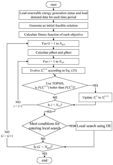
Figure 1.
Proposed method flowchart.
4. Experimental Results and Analysis
An experimental design for the proposed SSO-DE algorithm in this study is conducted in Section 4.1 to find out the best parameters of this algorithm for the CCHP optimization problem. The parameter setting and experimental situation of other algorithms are explained in Section 4.2. Finally, in Section 4.3, experimental results are detailed, represented, and compared among the proposed SSO-DE and other algorithms.
4.1. Experimental Design
The proposed SSO-DE in this research has seven parameters (factors) that need to be set, which are cg, cp, and cw in SSO as well as the mutation factor (CR), evolution parameter (F), and Y percentage of the good solutions entered the local search for every Z iteration. If all the parameters are explored for the experimental design, such a huge number of experiments is really not feasible assuming that each factor has three levels in which one must perform 37 = 2187 experiments. Therefore, the three parameters of SSO including cg, cp, and cw were set as one factor and the other parameters of DE were set as another factor so that the statistical analysis two-way ANOVA of two factors and three levels is performed.
The three levels of SSO parameter setting as shown in following Table 9 are all parameters that performed relatively well in the experimental testing process of this research.
Table 9.
Three levels of SSO parameter setting.
In order to enable the DE to be updated quickly and effectively in the early stage of the algorithm, we increased the diversity of the solution space in the middle and late stages, and increased the probability of jumping out of the space of the current solution; the parameter settings of DE in this research are as follows, Table 10.
Table 10.
Three levels of DE parameter setting.
This research used two-way ANOVA to analyze the two-way variance of parameter settings for the algorithm. However, three assumptions need to be satisfied, namely: the normality assumption, the independence assumption, and the homogeneity assumption, to use two-way ANOVA. It can ensure the independence of the data-collection process when designing the experiment. Thus, what this research needs to test is whether to meet the assumption of homogeneity and normality, and then use ANOVA analysis after confirming those are satisfied to find the best parameter setting for the experiment, which are shown in the following Section 4.1.1, Section 4.1.2 and Section 4.1.3 according to the three seasons including spring (autumn), summer, and winter.
4.1.1. Results of Experimental Design for Spring (Autumn) Data
The experimental data of spring and autumn are analyzed together according to references [25,60], in which most literature uses seasons as experimental data. The experimental data in spring (autumn) met the assumption of normality and the assumption of homogeneity as shown in Figure 2 and Figure 3. Therefore, two-way ANOVA can be used to analyze the variance of the two factors, and the results are shown in the following Table 11.
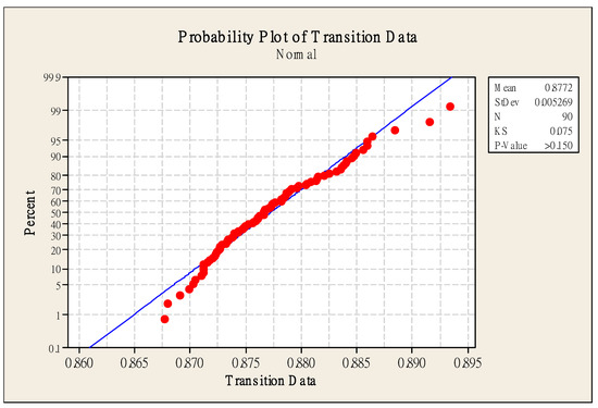
Figure 2.
Normality test for spring (autumn).
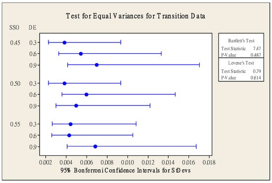
Figure 3.
Homogeneity test for spring (autumn).
Table 11.
Two-way ANOVA—transition.
The factor of parameter of SSO and factor of parameter of DE have no significant effect, and the interaction of the two factors has no significant effect according to the results of experimental design shown in Table 11. Thus, this study intends to use principal factor analysis, and the results are shown in the following, Figure 4, to determine the parameter configuration of the experimental data for winter.
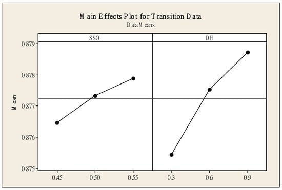
Figure 4.
Main effects plot for spring (autumn).
The parameters of DE were set to level 3 that is Y = 0.9 and initial F = 0.15 and the parameters of SSO were set to level 3, that is, cg = 0.55, cp = 0.35, and cw = 0.05 when it is in progress for the experimental data of spring (autumn) according to Figure 4. The parameter configuration is used in the subsequent experiment for spring (autumn) in Section 4.2.
4.1.2. Results of Experimental Design for Summer Data
The experimental data in summer do not meet the assumption of normality as shown in Figure 5; thus, the ANOVA can be used to analyze the variance of two factors. This study adopted Friedman’s test, which is a nonparametric method that does not need to satisfy the assumption of normality, to find the best parameter settings for DE and SSO. The results are shown in following Table 12 and Table 13.
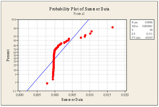
Figure 5.
Normality test for summer.
Table 12.
Friedman’s test, summer—DE blocked by SSO.
Table 13.
Friedman’s test, summer—SSO blocked by DE.
The parameters of DE were set to level 3, that is, Y = 0.9 and initial F = 0.15 and the parameters of SSO were set to level 2, that is, cg = 0.5, cp = 0.4, and cw = 0.05 when it is in progress for the experimental data of summer according to the analysis results obtained from Table 12 and Table 13. The parameter configuration is used in the subsequent experiment for summer in Section 4.2.
4.1.3. Results of Experimental Design for Winter Data
The experimental data in winter do not meet the assumption of normality as shown in Figure 6; w thus, the ANOVA can be used to analyze the variance of two factors. This study adopted Friedman’s test, which is a nonparametric method that does not need to satisfy the assumption of normality, to find the best parameter settings for DE and SSO. The results are shown in the following Table 14 and Table 15.
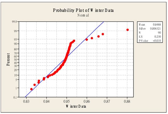
Figure 6.
Normality test for winter.
Table 14.
Friedman’s test, winter—DE blocked by SSO.
Table 15.
Friedman’s test, winter—SSO blocked by DE.
The parameters of DE were set to level 3, that is, Y = 0.9 and initial F = 0.15 and the parameters of SSO were set to level 1, that is, cg = 0.45, cp = 0.4, and cw = 0.1 when it is in progress for the experimental data of winter according to the analysis results obtained from Table 14 and Table 15. The parameter configuration is used in the subsequent experiment for winter in Section 4.2.
4.2. Experimental Situation
The experimental scenarios of this study are the energy load data of local residents in spring (autumn), summer, and winter; hence, there are three sets of experimental modules in this research. The experimental results obtained by the proposed SSO-DE were compared with those found by other algorithms including hybrid of PSO-DE, hybrid of ABC-DE, and hybrid of iSSO-DE. The four abovementioned algorithms all execute 200 iterations in different seasonal data as the stopping conditions of the algorithm and repeat the test 10 times to obtain the average, best, worst, standard deviation, and running time of the fitness value. The experiment used python3.7.1 to write the program, equipped with AMD Ryzen5 1600 CPU, 16 GB RAM, and a GTX1060 graphics card; the parameter settings of all algorithms are based on the computer environment test used in this research and the parameter settings with better experimental results in the process of the experiment are shown in the following Table 16.
Table 16.
Parameter configuration of each algorithm.
Before the experiment, this study first used SSO alone to compare with SSO-DE by various CR values set in order to verify the effectiveness of using DE in SSO-DE for local search. In three different seasons of data, each setting was set to 150 particles, 200 iterations, and 10 repeated experiments. The parameter configuration of SSO adopted the best parameter setting of each season in the experimental design of the previous section and the difference lies in the parameter settings of DE, which were uniformly set to Y = 100% and F = 0.1 + 0.0005 × Ngen. The settings are as shown in Table 17.
Table 17.
Parameter settings for SSO-DE.
The comparison results of SSO and SSO-DE in each season and the box and whisker diagrams are shown in Table 18, Table 19 and Table 20, where each method represents different algorithms, CR is the evolution parameter for DE, best is the best fitness value obtained by the algorithm in ten repeated experiments, worst is the worst fitness value, mean is the average fitness value of ten repeated experiments, and, finally, std represents its standard deviation, Figure 7, Figure 8 and Figure 9, respectively.
Table 18.
Comparison of SSO and SSO-DE for spring (autumn).
Table 19.
Comparison of SSO and SSO-DE for summer.
Table 20.
Comparison of SSO and SSO-DE for winter.
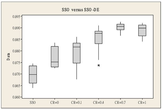
Figure 7.
Box and whisker diagram of SSO and SSO-DE for spring (autumn). *: Outliers.
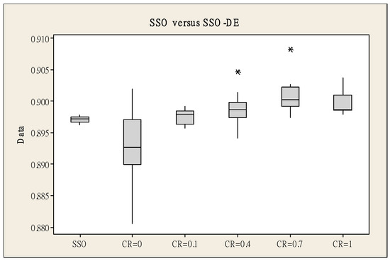
Figure 8.
Box and whisker diagram of SSO and SSO-DE for summer. *: Outliers.
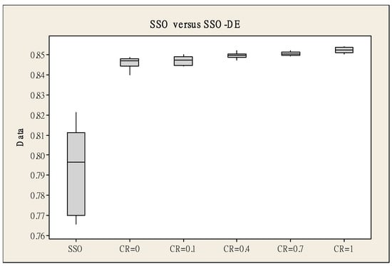
Figure 9.
Box and whisker diagram of SSO and SSO-DE for winter.
In spring (autumn) and winter, the difference in performance between SSO and SSO-DE was very obvious, that is, the calculation efficiency of SSO-DE was far superior to SSO regardless of the setting of the CR value of DE. In the summer experiment, the performance of SSO-DE was also slightly better than SSO although the gap of difference in performance was not as huge as those in spring (autumn) and winter. In addition, the setting of the CR value of DE in SSO-DE between 0.7 and 1 had the most eye-catching performance. These are the reasons that the initial CR value in the previous section of the experimental design was set to 0.85 and gradually increased to 0.95 with the number of iterations.
4.3. Experimental Results
The experimental results are shown in following Table 21, Table 22, Table 23, Table 24 and Table 25, where method represents different algorithms, aver.t is the average running time for each algorithm to perform 10 repeated experiments and its unit is seconds, best is the best fitness value obtained by the algorithm in 10 repeated experiments, worst is the worst fitness value, mean is the average fitness value of ten repeated experiments, and, finally, std represents its standard deviation.
Table 21.
Experiment results for spring (autumn).
Table 22.
Experiment results for summer.
Table 23.
Experiment results for winter.
Table 24.
Experiment results of Friedman’s test.
Table 25.
Experimental results of Dunnett’s test.
For the spring (autumn) experimental data, the experimental results of each algorithm are shown in Table 21 and Figure 10. The results showed that SSO-DE had the best performance in terms of average running time. SSO-DE also outperformed other algorithms in terms of best fitness value and average fitness value, although the performance of SSO-DE in the worst fitness value was slightly lower than that of ABC-DE. Overall, SSO-DE performed the best in the spring (autumn) experimental data set.
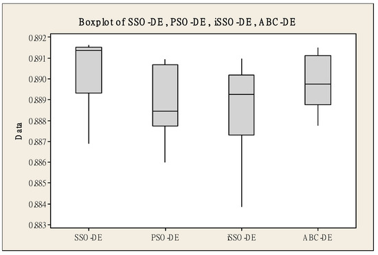
Figure 10.
Box and whisker diagram for spring (autumn).
For the summer experimental data, the experimental results of each algorithm are shown in Table 22 and Figure 11. The results showed that SSO-DE had the best performance in terms of average running time. ABC-DE had the best performance and SSO-DE has the second-best performance in terms of best fitness value, worst fitness value, and average fitness value and PSO-DE had the best performance in terms of std. ABC-DE took the longest running time. Thus, SSO-DE also performed quite well in the summer experimental data set.
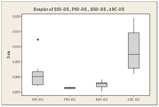
Figure 11.
Box and whisker diagram for summer. *: Outliers.
For the winter experimental data, the experimental results of each algorithm are shown in Table 23 and Figure 12. The results showed that SSO-DE had the best performance in terms of average running time. In addition, SSO-DE had the best performance in terms of best fitness value, worst fitness value, and average fitness value. Thus, SSO-DE had the most eye-catching performance in the winter experimental data set.
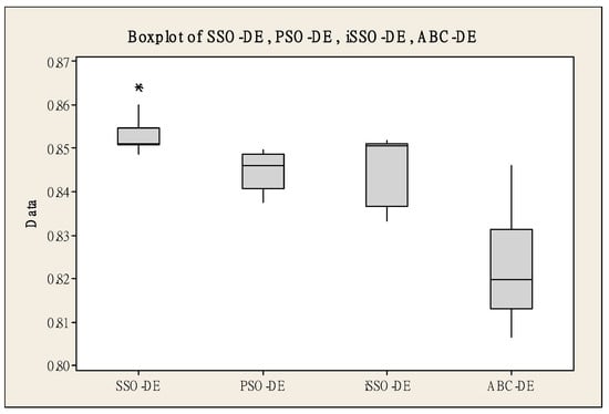
Figure 12.
Box and whisker diagram for winter. *: Outliers.
The Freidman test results of the four algorithms for the abovementioned experiments of three seasons are shown in following Table 24. The p-value was 0.000, which represents a significant difference in fitness values between different algorithms. Additionally, in terms of sum of ranks, it could be found that the sum of ranks value of SSO-DE was the largest, which shows the fitness performance of SSO-DE was the best among all algorithms in the experiments of the three seasons.
Furthermore, the Dunnett’s test (post-hoc test) experimental results of the four algorithms including ABC-DE, iSSO-DE, PSO-DE, and the proposed SSO-DE in the three seasonal data experiments are shown in Table 25. The results showed that there was no significant difference between the other three algorithms with SSO-DE but the p-value compared with PSO-DE was very close to 0.05. The reason for this result should be that the fitness value performance of SSO-DE in the summer experiment is slightly inferior to that of ABC-DE and the standard deviation performance of SSO-DE is not as stable as that of PSO-DE. Although the experimental data in the three seasons obtained by SSO-DE performed better than those found by PSO-DE and iSSO-DE, the difference is not particularly significant as shown by Dunnett’s test. However, in the three data sets, the running time of SSO-DE was much shorter than other compared algorithms, and Friedman’s test in the previous paragraph also confirmed that the comprehensive performance of SSO-DE was the best.
5. Conclusions
This study proposed a new algorithm called SSO-DE, which combined a differential evolution (DE) algorithm as the local search strategy with simplified swarm optimization (SSO) to solve the optimization problem of CCHP combined with renewable energy. In addition, this study used the TOPSIS method to convert the original multi-objective optimization problem, including minimizing the operation cost, minimizing the carbon emissions, and maximizing the energy utilization rate, into a single-objective optimization problem to reduce the calculation steps and increase the efficiency of the solution. Moreover, this work studied the CCHP based on Xikou village, Lieyu township, Kinmen county, Taiwan as an experimental case to realize the CCHP-combined-with-microgrid system of renewable energy and help to solve the problem that most of the research on CCHP is limited to construction such as hotels and hospitals. The experimental results obtained by the proposed SSO-DE were compared with POS-DE, iSSO-DE, and ABC-DE, and the numerical results are as follows:
- For the spring (autumn) experimental data set, SSO-DE performed the best in terms of best fitness value, average fitness value, and average running time.
- For the summer experimental data, SSO-DE performed the best in terms of average running time. ABC-DE had the best performance and SSO-DE had the second-best performance in terms of best fitness value, worst fitness value, and average fitness value.
- For the winter experimental data, SSO-DE performed the best in terms of best fitness value, worst fitness value, average fitness value, and average running time.
- The results of the Friedman test showed that the proposed SSO-DE had the best comprehensive performance among all experimental modules including spring (autumn), summer, and winter. In addition, SSO-DE had the lowest running time in all experiments.
- The results of Dunnett’s test (post-hoc test) showed that there was no significant difference between the other three algorithms with SSO-DE. The reason for this result should be that the fitness value performance of SSO-DE in the summer experiment is slightly inferior to that of ABC-DE and the standard deviation performance of SSO-DE is not as stable as that of PSO-DE.
However, in the three data sets, the running time of SSO-DE was much shorter than other compared algorithms, and Friedman’s test in the previous paragraph also confirmed that the comprehensive performance of SSO-DE is the best.
Author Contributions
Conceptualization, W.-C.Y., W.Z., Y.-F.P. and C.-L.H.; methodology, W.-C.Y., W.Z., Y.-F.P. and C.-L.H.; software, W.-C.Y., W.Z., Y.-F.P. and C.-L.H.; validation, W.-C.Y., W.Z. and Y.-F.P.; formal analysis, W.-C.Y., W.Z., Y.-F.P. and C.-L.H.; investigation, W.-C.Y., W.Z. and Y.-F.P.; resources, W.-C.Y., W.Z. and Y.-F.P.; data curation, W.-C.Y., W.Z. and Y.-F.P.; writing—original draft preparation, W.-C.Y., W.Z., Y.-F.P. and C.-L.H.; writing—review and editing, W.-C.Y., W.Z., Y.-F.P. and C.-L.H.; visualization, W.-C.Y. and W.Z.; supervision, W.-C.Y.; project administration, W.-C.Y.; funding acquisition, W.Z. All authors have read and agreed to the published version of the manuscript.
Funding
This research was supported in part by National Natural Science Foundation of China (Grant No. 621060482), Research and Development Projects in Key Areas of Guangdong Province (Grant No. 2021B0101410002) and National Science and Technology Council, R.O.C (MOST 107-2221-E-007-072-MY3, MOST 110-2221-E-007-107-MY3, MOST 109-2221-E-424-002 and MOST 110-2511-H-130-002).
Acknowledgments
We wish to thank the anonymous editor and the referees for their constructive comments and recommendations, which significantly improved this paper. This article was once submitted to arXiv as a temporary submission that was just for reference and did not provide the copyright.
Conflicts of Interest
The authors declare no conflict of interest.
Abbreviations, Symbols, and Indicators
| Abbreviations | Definition |
| AC | Absorption Chiller |
| CCHP | Combined Cooling, Heating and Power system |
| ES | Electricity-Storage Device |
| EC | Electric Chiller |
| FTL | Following Thermal Loading |
| FEL | Following Electric Loading |
| GT | Gas Turbine |
| GB | Gas Boiler |
| Grid | Main grid |
| HS | Heating-Storage Device |
| NG | Natural Gas |
| OM | Operation Cost |
| PV | Photovoltaic |
| recy | Recycled thermal |
| WT | Wind Turbine |
| Symbols | Definition |
| C | Cold energy (Kwh) |
| COP | Coefficient of refrigeration |
| E | Stored electric energy (Kwh) |
| f | Objective function for multi-objective optimization |
| F1 | Economic cost (NTD) |
| F2 | Pollution cost (KG) |
| F3 | Energy utilization rate (%) |
| FNG | Fuel cost (NTD/KG) |
| H | Stored heat (Kwh) |
| J | Electricity price (NTD/Kwh) |
| K | Operating cost of unit power generation (NTD/Kwh) |
| P | Electricity (Kwh) |
| Pr | Price (NTD/) |
| Q | Thermal energy (Kwh) |
| R | Total energy (Kwh) |
| u | Power generation efficiency (kg/kWh) |
| V | Capacity (Kwh) |
| η | Energy conversion rate |
| σ | Energy-storage loss rate of energy-storage equipment |
| γ | Loss rate when energy-storage device releases or stores energy |
| Indicators | Definition |
| c | charge |
| d | discharge |
| j | Machine type, such as PV, WT, GB, etc. |
| t | hour |
References
- Ali, Z.M.; Aleem, S.H.E.A.; Omar, A.I.; Mahmoud, B.S. Economical-Environmental-Technical Operation of Power Networks with High Penetration of Renewable Energy Systems Using Multi-Objective Coronavirus Herd Immunity Algorithm. Mathematics 2022, 10, 1201. [Google Scholar] [CrossRef]
- Rawa, M.; Abusorrah, A.; Bassi, H.; Mekhilef, S.; Ali, Z.M.; Aleem, S.H.E.A.; Hasanien, H.M.; Omar, A.I. Economical-technical-environmental operation of power networks with wind-solar-hydropower generation using analytic hierarchy process and improved grey wolf algorithm. Ain Shams Eng. J. 2021, 12, 2717–2734. [Google Scholar] [CrossRef]
- Omar, A.I.; Ali, Z.M.; Al-Gabalawy, M.; Aleem, S.H.E.A.; Al-Dhaifallah, M. Multi-Objective Environmental Economic Dispatch of an Electricity System Considering Integrated Natural Gas Units and Variable Renewable Energy Sources. Mathematics 2020, 8, 1100. [Google Scholar] [CrossRef]
- Jha, S.K.; Bilalovic, J.; Jha, A.; Patel, N.; Zhang, H. Renewable energy: Present research and future scope of Artificial Intelligence. Renew. Sustain. Energy Rev. 2017, 77, 297–317. [Google Scholar] [CrossRef]
- BP Statistical Review of World Energy. Available online: https://large.stanford.edu/courses/2018/ph241/kumar2/docs/bp-2018.pdf (accessed on 11 January 2021).
- Chang, Y.R.; Jiang, J.L.; Lee, Y.D. The Perspective of Microgrid Technology Development. J. Taiwan Energy 2015, 2, 259–278. [Google Scholar]
- Yang, H.; Lu, L.; Zhou, W. A novel optimization sizing model for hybrid solar-wind power generation system. Sol. Energy 2007, 81, 76–84. [Google Scholar] [CrossRef]
- Atwa, Y.M.; El-Saadany, E.F.; Salama, M.M.A.; Seethapathy, R. Optimal renewable resources mix for distribution system energy loss minimization. IEEE Trans. Power Syst. 2010, 25, 360–370. [Google Scholar] [CrossRef]
- Ning, Y.; Li, X.; Ma, X.; Jia, X.; Hui, D. Optimal schedule strategy of battery energy storage systems for peak load shifting based on interior point method. In Proceedings of the 2016 12th World Congress on Intelligent Control and Automation (WCICA), Guilin, China, 12–15 June 2016. [Google Scholar]
- Sigrist, L.; Lobato, E.; Rouco, L. Energy storage systems providing primary reserve and peak shaving in small isolated power systems: An economic assessment. Int. J. Electr. Power Energy Syst. 2013, 53, 675–683. [Google Scholar] [CrossRef]
- Cho, H.; Mago, P.J.; Luck, R.; Chamra, L.M. Evaluation of CCHP systems performance based on operational cost, primary energy consumption, and carbon dioxide emission by utilizing an optimal operation scheme. Appl. Energy 2009, 86, 2540–2549. [Google Scholar] [CrossRef]
- Cho, H.; Smith, A.D.; Mago, P. Combined cooling, heating and power: A review of performance improvement and optimization. Appl. Energy 2014, 136, 168–185. [Google Scholar] [CrossRef]
- Fu, L.; Zhao, X.L.; Zhang, S.G.; Jiang, Y.; Li, H.; Yang, W.W. Laboratory research on combined cooling, heating and power (CCHP) systems. Energy Convers. Manag. 2009, 50, 977–982. [Google Scholar] [CrossRef]
- Abdollahi, G.; Meratizaman, M. Multi-objective approach in thermos environomic optimization of a small-scale distributed CCHP system with risk analysis. Energy Build. 2011, 43, 3144–3153. [Google Scholar] [CrossRef]
- Wang, J.J.; Jing, Y.Y.; Zhang, C.F. Optimization of capacity and operation for CCHP system by genetic algorithm. Appl. Energy 2010, 87, 1325–1335. [Google Scholar] [CrossRef]
- Chen, S.B. Assessment of Autonomous Renewable Energy System for Kinmen. Master’s Thesis, National Digital Library of Theses and Dissertations, Taipei, Taiwan, 2013. [Google Scholar]
- Mago, P.; Fumo, N.; Chamra, L. Performance analysis of CCHP and CHP systems operating following the thermal and electric load. Int. J. Energy Res. 2009, 33, 852–864. [Google Scholar] [CrossRef]
- Li, L.; Mu, H.; Li, N.; Li, M. Analysis of the integrated performance and redundant energy of CCHP systems under different operation strategies. Energy Build. 2015, 99, 231–242. [Google Scholar] [CrossRef]
- Fang, F.; Wang, Q.H.; Shi, Y. A novel optimal operational strategy for the CCHP system based on two operating modes. IEEE Trans. Power Syst. 2011, 27, 1032–1041. [Google Scholar] [CrossRef]
- Xu, D.; Qu, M. Energy, environmental, and economic evaluation of a CCHP system for a data center based on operational data. Energy Build. 2013, 67, 176–186. [Google Scholar] [CrossRef]
- Hasan, R.A.; Shahab, S.N.; Ahmed, M.A. Correlation with the fundamental PSO and PSO modifications to be hybrid swarm optimization. Iraqi J. Comput. Sci. Math. 2021, 2, 25–32. [Google Scholar] [CrossRef]
- Aggarwal, K.; Mijwil, M.M.; Sonia Al-Mistarehi, A.-H.; Alomari, S.; Gök, M.; Alaabdin, A.M.Z.; Abdulrhman, S.H. Has the Future Started? The Current Growth of Artificial Intelligence, Machine Learning, and Deep Learning. Iraqi J. Comput. Sci. Math. 2022, 3, 115–123. [Google Scholar] [CrossRef]
- Soheyli, S.; Mayam, M.H.S.; Mehrjoo, M. Modeling a novel CCHP system including solar and wind renewable energy resources and sizing by a CC-MOPSO algorithm. Appl. Energy 2016, 184, 375–395. [Google Scholar] [CrossRef]
- Wang, J.; Yang, Y.; Mao, T.; Sui, J.; Jin, H. Life cycle assessment (LCA) optimization of solar-assisted hybrid CCHP system. Appl. Energy 2015, 146, 38–52. [Google Scholar] [CrossRef]
- Li, G.; Wang, R.; Zhang, T.; Ming, M. Multi-Objective Optimal Design of Renewable Energy Integrated CCHP System Using PICEA-g. Energies 2018, 11, 743. [Google Scholar] [CrossRef]
- Wu, J.; Wang, J.; Li, S. Multi-objective optimal operation strategy study of micro-CCHP system. Energy 2012, 48, 472–483. [Google Scholar] [CrossRef]
- Gimelli, A.; Muccillo, M.; Sannino, R. Optimal design of modular cogeneration plants for hospital facilities and robustness evaluation of the results. Energy Convers. Manag. 2017, 134, 20–31. [Google Scholar] [CrossRef]
- Yousefi, H.; Ghodusinejad, M.H.; Noorollahi, Y. GA/AHP-based optimal design of a hybrid CCHP system considering economy, energy and emission. Energy Build. 2017, 138, 309–317. [Google Scholar] [CrossRef]
- Yeh, W.C. A two-stage discrete particle swarm optimization for the problem of multiple multi-level redundancy allocation in series systems. Expert Syst. Appl. 2009, 36, 9192–9200. [Google Scholar] [CrossRef]
- Li, Y.; Wu, J.; Yan, H.; Li, D.; Ma, T.; Lin, K. Multi-objective optimal operation of combined cooling, heating and power microgrid. In Proceedings of the 2017 IEEE Conference on Energy Internet and Energy System Integration (EI2), Beijing, China, 26–28 November 2017. [Google Scholar]
- Taipower Company. Available online: https://www.taipower.com.tw/tc/page.aspx?mid=96.2020 (accessed on 11 January 2021).
- Environment Protection Bureau. 2013. Available online: https://kepb.kinmen.gov.tw/News_Content.aspx?n=C326FCC8544D820C&sms=4FEFD09995C4BB81&s=C3546D66725495D1 (accessed on 1 February 2021).
- Bureau of Energy, Ministry of Economic Affairs. 2020. Available online: https://www.moeaboe.gov.tw/ECW/populace/content/SubMenu.aspx?menu_id=2224 (accessed on 1 February 2021).
- Kuo, P.Y. A Study on Electrical Consumption Survey and Evaluation System of Residential Buildings. Ph.D. Thesis, National Cheng Kung University, Tainan City, Taiwan, 2005. [Google Scholar]
- Bureau TCM. 2020. Available online: https://opendata.cwb.gov.tw/index (accessed on 11 January 2021).
- Zeng, J.; Xu, D.D.; Liu, J.F.; Li, C. Multi-objective Optimal Operation of Microgrid Considering Dynamic Loads. In Proceedings of the CSEE, Dallas, TX, USA, 5–6 April 2016; Volume 36. [Google Scholar]
- Shih, H.S.; Shyur, H.J.; Lee, E.S. An extension of TOPSIS for group decision making. Math. Comput. Model. 2007, 45, 801–813. [Google Scholar] [CrossRef]
- Yeh, W.C.; Chang, W.W.; Chung, Y.Y. A new hybrid approach for mining breast cancer pattern using discrete particle swarm optimization and statistical method. Expert Syst. Appl. 2009, 36, 8204–8211. [Google Scholar] [CrossRef]
- Yeh, W.C. Optimization of the disassembly sequencing problem on the basis of self-adaptive simplified swarm optimization. IEEE Trans. Syst. Man Cybern. Part A Syst. Hum. 2012, 42, 250–261. [Google Scholar] [CrossRef]
- Huang, C.L.; Jiang, Y.; Yeh, W.C. Developing Model of Fuzzy Constraints Based on Redundancy Allocation Problem by an Improved Swarm Algorithm. IEEE Access 2020, 8, 155235–155247. [Google Scholar] [CrossRef]
- Yeh, W.C. A New Exact Solution Algorithm for a Novel Generalized Redundancy Allocation Problem. Inf. Sci. 2017, 408, 182–197. [Google Scholar] [CrossRef]
- Yeh, W.C. Solving cold-standby reliability redundancy allocation problems using a new swarm intelligence algorithm. Appl. Soft Comput. 2019, 83, 105582. [Google Scholar] [CrossRef]
- Yeh, W.C. A Novel Boundary Swarm Optimization for Reliability Redundancy Allocation Problems. Reliab. Eng. Syst. Saf. 2019, 192, 106060. [Google Scholar] [CrossRef]
- Yeh, W.C.; Zhu, W.; Tan, S.Y.; Wang, G.G.; Yeh, Y.H. Novel General Active Reliability Redundancy Allocation Problems and Algorithm. Reliab. Eng. Syst. Saf. 2021, 218, 108167. [Google Scholar] [CrossRef]
- Huang, C.L.; Jiang, Y.; Yeh, W.C. Solving Cold-standby Reliability Redundancy Allocation Problems with Particle-based Simplified Swarm Optimization. J. Sens. 2021, 2021, 7833641. [Google Scholar] [CrossRef]
- Lin, H.C.S.; Huang, C.L.; Yeh, W.C. A Novel Constraints Model of Credibility-Fuzzy for Reliability Redundancy Allocation Problem by Simplified Swarm Optimization. Appl. Sci. 2021, 11, 10765. [Google Scholar] [CrossRef]
- Yeh, W.C.; Lin, J.S. New parallel swarm algorithm for smart sensor systems redundancy allocation problems in the Internet of Things. J. Supercomput. 2018, 74, 4358–4384. [Google Scholar] [CrossRef]
- Yeh, W.C.; Tan, S.Y. Simplified Swarm Optimization for the Heterogeneous Fleet Vehicle Routing Problem with Time-Varying Continuous Speed Function. Electronics 2021, 10, 1775. [Google Scholar] [CrossRef]
- Tan, S.Y.; Yeh, W.C. The Vehicle Routing Problem: State-of-the-Art Classification and Review. Appl. Sci. 2021, 11, 10295. [Google Scholar] [CrossRef]
- Yeh, W.C.; Liu, Z.; Yang, Y.C.; Tan, S.Y. Solving Dual-Channel Supply Chain Pricing Strategy Problem with Multi-Level Programming Based on Improved Simplified Swarm Optimization. Technologies 2022, 10, 73. [Google Scholar] [CrossRef]
- Zhu, W.; Huang, C.L.; Yeh, W.C.; Jiang, Y.; Tan, S.Y. A Novel Bi-Tuning SSO Algorithm for Optimizing the Budget-Limited Sensing Coverage Problem in Wireless Sensor Networks. Appl. Sci. 2021, 11, 10197. [Google Scholar] [CrossRef]
- Yeh, W.C.; Jiang, Y.; Tan, S.Y.; Yeh, C.Y. A New Support Vector Machine Based on Convolution Product. Complexity 2021, 2021, 9932292. [Google Scholar] [CrossRef]
- Wu, T.Y.; Jiang, Y.Z.; Su, Y.Z.; Yeh, W.C. Using Simplified Swarm Optimization on Multiloop Fuzzy PID Controller Tuning Design for Flow and Temperature Control System. Appl. Sci. 2020, 10, 8472. [Google Scholar] [CrossRef]
- Yeh, W.C.; Jiang, Y.; Huang, C.L.; Xiong, N.N.; Hu, C.F.; Yeh, Y.H. Improve Energy Consumption and Signal Transmission Quality of Routings in Wireless Sensor Networks. IEEE Access 2020, 8, 198254–198264. [Google Scholar] [CrossRef]
- Yeh, W.C. A new harmonic continuous simplified swarm optimization. Appl. Soft Comput. 2019, 85, 105544. [Google Scholar] [CrossRef]
- Yeh, W.C.; Lai, C.M.; Tseng, K.C. Fog computing task scheduling optimization based on multi-objective simplified swarm optimization. J. Phys. Conf. Ser. 2019, 1411, 012007. [Google Scholar] [CrossRef]
- Yeh, W.C. A squeezed artificial neural network for the symbolic network reliability functions of binary-state networks. IEEE Trans. Neural Netw. Learn. Syst. 2017, 28, 2822–2825. [Google Scholar] [CrossRef]
- Yeh, W.C.; Wei, S.C. Economic-based resource allocation for reliable Grid-computing service based on Grid Bank. Future Gener. Comput. Syst. 2012, 28, 989–1002. [Google Scholar] [CrossRef]
- Lee, W.C.; Chuang, M.C.; Yeh, W.C. Uniform parallel-machine scheduling to minimize makespan with position-based learning curves. Comput. Ind. Eng. 2012, 63, 813–818. [Google Scholar] [CrossRef]
- Wu, T.; Mai, W.; Qin, M.; Zhang, C.; Li, J.; Nie, Y.; Liu, J.; Chung, C.Y. Optimal operation of combined cooling heat and power microgrid with PEVs. In Proceedings of the 2015 IEEE Eindhoven PowerTech, Eindhoven, The Netherlands, 29 June–2 July 2015. [Google Scholar]
Publisher’s Note: MDPI stays neutral with regard to jurisdictional claims in published maps and institutional affiliations. |
© 2022 by the authors. Licensee MDPI, Basel, Switzerland. This article is an open access article distributed under the terms and conditions of the Creative Commons Attribution (CC BY) license (https://creativecommons.org/licenses/by/4.0/).