Abstract
Tracked inspection robots possess prominent advantages in dealing with severe environment rescue, safety inspection, and other important tasks, and have been used widely. However, tracked robots are affected by skidding and slipping, so it is difficult to achieve accurate control. For example, the control parameters of a tracked robot are the same during driving, but the pressure, shear force and steering resistance of the robot on the road surface are different, which affects the steering characteristics of the robot on complex terrain. Based on analysis of the structural parameters and steering radius of the robot, the traction force and resistance torque models of the tracked robot were established, and the plane dynamics of the robot’s steering were analyzed and solved. The corresponding relationships between the road parameters, relative steering radius, and lateral relative offset of the robot on three typical roads were obtained. Mathematical models of the robot’s track speed and relative steering radius with and without skid and slip were established. Through simulation analysis of Matlab software, the corresponding relationship between the relative steering radius of the robot and the velocity difference of the two tracks were obtained. Taking angular obstacles as an example, three obstacle-avoidance steering control strategies, once turning in situ center, twice turning in situ center, and large-radius steering were developed. The tracked robot and obstacle multi-body dynamic simulation models were constructed using ADAMS simulation software. The simulation results show that all three methods can complete the steering tasks according to the requirements; however, under the influence of skid and slip, the trajectory of the robot deviates from the ideal trajectory, which has a great impact on large-radius steering, even though the large-radius obstacle-avoidance steering control strategy has the advantages of a smooth trajectory, fast steering speed, and high efficiency. The obstacle-avoidance steering experiments were completed by the robot prototype, which verifies the rationality of robot steering theory, which could provide the corresponding theoretical basis for autonomous obstacle-avoidance navigation control of a tracked robot.
1. Introduction
As an important piece equipment for underground inspection in coal mines, inspection robots undertake safety inspection under various working conditions and have been used widely. In particular, tracked robots have been applied in many complex environments because of their good performance in obstacle climbing and environmental adaptability [1]. However, the control performance of a tracked robot is relatively poor compared to that of a wheeled robot; therefore, it is difficult to achieve accurate control of a tracked robot. The obstacle avoidance control strategies of tracked robots should be studied in depth.
Obstacle avoidance strategies have been studied in many fields, especially in the fields of robotics and cooperative robotics science. Boschetti G. studied the influence of collision avoidance strategies on human–robot collaborative systems; its strategies can mitigate the impact of decreasing system performance by increasing the cooperation area [2]. Cecilia S. studied avoidance strategy for redundant manipulators in a simulation environment, her algorithm had been implemented in a 2D environment for a 3R planar manipulator [3]. Maurizio F. studied the influence of the product characteristics on human–robot collaboration and developed an algorithm that simulates product assembly in the considered workspace [4]. David J. studied the acceleration obstacle as a concept to enable a robot’s navigation in human crowds [5]. Muhammad A. proposed a novel control architecture that can ensure the safety of robots working in close proximity to humans in dynamically changing environments and demonstrated their approach on a seven degree-of-freedom Kuka LBR iiwa robotic manipulator [6]. Felix F. developed a generic probabilistic framework for adapting ProMPs and demonstrated their approach in a dual-robot-arm setting [7]. Dai Y. proposed that obstacle avoidance and trajectory planning is the basis of robotic arm motion and that it has an essential impact on the quality of the operation to be completed [8].
In research on the structural design and control method of tracked robots, some scholars have deeply studied the steering control of tracked robots. For example, Steeds [9] made an earlier study on this issue. In his pioneering analysis, the coefficient of friction was isotropic, and the frictional force was acting opposite to the relative motion of the track with respect to the ground. Wong [10] expanded the work of his predecessors. His general theory was derived from a detailed analysis of the relationship between shear stress-displacement in track–ground interaction. Dong C. established a steering mechanics model of an articulated tracked vehicle and determined the kinematics and mechanics-related parameters in its steering process of articulated tracked vehicles [11]. Gai J. studied the steering control strategy of electric-driven vehicles through the track’s skid and slip, which can reduce the influence of the track’s skid and slip on the kinematic control of electric-driven vehicles during vehicle steering [12]. Gao Q. designed a steering device for an unmanned agricultural power chassis by compensating the power differential steering with a motor and realized the in-place steering of the chassis [13]. Guan Z. established the relationship between the steering slip rate of high- and low-speed side tracks and steering-related parameters, built a steering motion parameter test system for a tracked combine harvester, and completed the field experiment. [14]. Dai Y. constructed a multibody dynamics model of a submarine tracked collector and realized an integrated construction and linkage simulation of the multibody dynamics model of the entire deep-sea mining system [15]. Han Z., in order to further improve the adaptability of the crawler chassis under complex driving road conditions, used the topographic and geomorphological characteristics of the hillside orchard to carry out slope trafficability analysis of the tracked chassis [16].
The trajectory-tracking control of a tracked robot with nonholonomic constraints resembles that of wheeled robot, which has become a focus of research interest. When a tracked robot turns, its ability is usually poor due to the large sliding degree of the track, which is more obvious in the skid and slip of the two tracks. The above literature shows that tracked robots are applied in all industries, but under different road conditions, and although the control parameters of tracked robots are the same, the pressure, shear force generated by tracked robots on the road surface, and steering resistance of the robot on the ground are different, which affects the steering characteristics of the robot [17]. The track–ground interaction is important for predicting the turning resistance of tracked robot [18]. Therefore, it is necessary to further study the steering mechanism of the tracked robot and formulate the corresponding control strategy according to the road environment, its own structural characteristics, and its own driving parameters for completing driving control tasks [19]. To realize autonomous navigation of tracked robots in complex environments, it is necessary to quantitatively analyze the steering of the tracked robot and determine its control parameters to actively avoid obstacles on different roads.
The paper is organized as follows: Firstly, the structure, the skid and slip rate, and the steering radius of a tracked robot were analyzed. Secondly, the kinematic and dynamic models of the tracked mobile robot were established. Thirdly, the rationality of obstacle-avoidance steering control strategies of the tracked robot were analyzed by simulation. Finally, a theoretical analysis structure was used to guide the tracked robot to complete the related performance tests.
2. Tracked Robot Structure
To adapt to complex working conditions, a tracked robot with four swing arms and six tracks was developed for this paper, which can be applied to daily inspection work in a coal mine [20]. The body structure of the tracked robot is shown in Figure 1. The related parameters of the tracked robot are listed in Table 1. The robot’s four swing arms were free to rotate by 360°. During the course of the tracked robot steering on a horizontal hard road, the contact area between the track of the swing-arm driving wheel and the road surface was small, which had little influence on the overall steering of the tracked robot. Therefore, the influence of the swing arm track on ground steering is ignored in the study of robot steering. When the tracked robot was driving on a soft and muddy road environment, the track of the swing-arm of the tracked robot had greater contact with the road surface, which had a greater influence on the driving trajectory of the robot. In this case, it was necessary to consider the influence of the swing-arm on the steering control of the tracked robot.
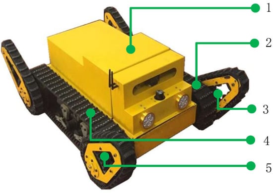
Figure 1.
Tracked robot with four swing arms and six tracks. 1. Body; 2. Left track; 3. Left driving wheel; 4. Right track; 5. Right driving wheel.

Table 1.
Main parameters of tracked robot.
The two motors of the tracked robot drove the driving wheels on both sides and then drove the driven wheels to rotate through the tracks. The tracked robot realized various motion controls by controlling the speed difference of the driving motors, such as linear motion and steering motion, with an arbitrary radius.
3. Kinetics of Tracked Robot during Steady-State Turning
3.1. Traction Force Analysis
To calculate the traction force of the robot track, the following assumptions were made.
- (1)
- The robot moves at a low and uniform speed on the horizontal ground.
- (2)
- When the robot is driving, the deformation resistance of the tracks on both sides is equal.
- (3)
- Ignoring the influence of track width, the tracks on both sides of the ground have an equal and symmetric appearance, and the pressure at the track contact area is equal and evenly distributed along the track-length direction of the robot.
- (4)
- The influence of the swing-arm track on the steering performance of the robot is ignored.
Therefore, the load per unit length of the robot track is:
where G is the weight of the robot and L is the length of the robot track in contact with ground.
The driving forces of the track interfere with each other while controlling tracked vehicles using driving force feedback. Therefore, the driving force distribution that decouples the driving forces must be considered [21,22]. During the steering process of the robot, there are many types of force on the track, and the different steering modes bear different forces. In Wong’s model, the shear forces at any point on the track–soil interface were assumed to have a direction opposite to that of the sliding velocity of that point with respect to the ground [23]. The force of the robot during steering is shown in Figure 2. During steering, the two tracks of the robot simultaneously provide traction. Point M of the track on the right side of the robot slipped during the steering process. The tangential force caused by sliding is opposite to the sliding velocity , and the component force in its y-direction constitutes the traction force of the robot. Consider a micro-element Dy at point M, and the tangential reaction force on this micro-element is proportional to the positive pressure per unit length. The traction force on the right track of the robot is:
where is the friction resistance coefficient ; , R is the steering radius, B is the distance between the center of the robot’s driving wheel tracks, and is the relative steering radius.
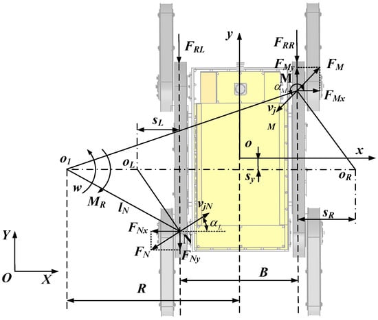
Figure 2.
Analysis diagram of robot steering force.
, and the above equation is integrated to obtain:
where , is the relative lateral offset of the right track.
Similarly, the traction force expression of the left track can be expressed as:
where and are the relative lateral offsets of the right track, and its negative sign indicates that it is in the opposite direction.
3.2. Analysis of the Torque of Skid-Steering
The steering resistance of the robot was a combination of the steering resistance moments of the two tracks. Because the center of gravity of the robot does not coincide with the center of its geometry, the steering axis of the robot moves the distance along its y-direction. The minute element is used for the right track, and the component force of the tangential reaction force in the x-direction is . Additionally, the steering resistance moment of the robot can be expressed as
where .
After integration of the above equation, it can be concluded that:
, , Equation (6) can be simplified as follows:
Similarly, the resistance moment of the right track can be obtained as follows:
It can be seen that in a certain environment, the resistance moment suffered by the robot during the steering process is not related to the longitudinal offset of the robot’s center of gravity; it is only related to the relative lateral offset of the instantaneous steering center of the robot’s tracks on both sides, and the negative sign indicates that the steering resistance of the robot is opposite to the specified direction. The total steering resistance moment of the robot track is
When and , the skid and slip rates of the robot are zero; that is, the influence of the robot’s skid and slip on the robot’s steering motion is not considered, and the motion at this time is the ideal steering motion, and .
3.3. Dynamics Analysis for Skid-Steering
According to the analysis of robot steering dynamics, it is known that the robot must meet the following conditions in the process of low-speed and uniform steering [12]:
To ensure that the tracked robot turns at a constant speed, the resultant force on the longitudinal track must be zero. The longitudinal traction force and of the robot and the lateral torque m of the robot track are functions of the lateral relative offsets and , respectively. In this study, ground deformation resistance in the steering process of the robot was replaced by ground deformation resistance when the robot was driving in a straight line, and the deformation resistances of the two tracks were equal, so . By substituting force and moment into the above equation, the following formula can be obtained:
where is the structural parameter of the robot.
It can be seen from the above formula that and are ground parameters and is the structural parameter of the robot. When the ground and structural parameters are determined, the equation contains only two unknowns, and , with a given relative radius, indicating that the system of equations has a solution.
3.4. Simulation Analysis for Lateral Relative Offset
The parameters of the three roads are listed in Table 2. In order to explore the corresponding relationship between the structural parameters, ground parameters, relative steering radius of the tracked robot and the relative deviation of the robot’s steering, the value range of the structural parameter of the robot is determined as . The relative steering radius is .
Table 2.
Typical road parameters.
In the case of a hard road surface, the corresponding relationship between the changes in , , , and was determined. It can be seen from Figure 3 that the lateral relative offset of the right track of the robot has a large range of variation under the condition of a certain hard road, whereas the of the left track is small. The lateral relative offset increases with an increase in the relative steering radius , whereas decreases with it; however, both and increase with the increase in .
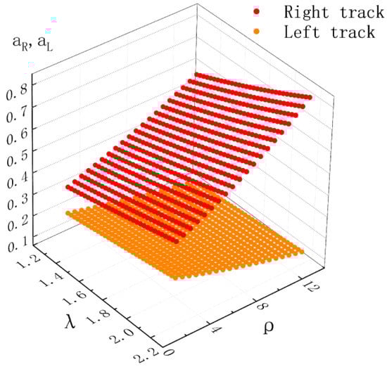
Figure 3.
The relationship between , , and .
In addition, when the steering angular velocity of the robot is constant, the larger the , the more severely the robot will skid. The energy of the robot is lost to the work consumed by the robot’s track skidding, which reduces its energy utilization rate. = 0.5~15, = 0.33~0.51 and = 0.11~0.21. To achieve a good turning effect, the structural parameter of the robot should be as small as possible. In this study, the structural parameter of the robot was set as mm, which meets the requirements.
When the robot drove on a hard road, the ground deformation coefficient and steering resistance coefficient of the road surface were determined, and the changes in the and of the robot under different road conditions were calculated. The road parameters were substituted into Equation (11).
As shown in Figure 4, when is small, the lateral relative offsets of the left and right tracks of the tracked robot do not differ significantly but are slightly different. will increase as and increase, and will decrease and . The difference between and increased as increased.
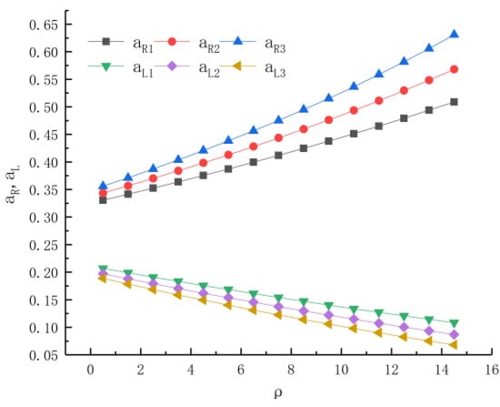
Figure 4.
Relationship between , and under typical road conditions.
4. Analysis of Steering Characteristics of Tracked Robot
4.1. Relationship between Angular Velocity and Steering Radius
When the body structure of the tracked robot is determined, the transmission relationship between the robot driving wheel motor and track wheel is also determined. When the linear velocity of the driving wheel is determined, the relationship between the relative steering radius, steering angular velocity of the robot, and driving parameters can be obtained as follows:
When the tracked robot turns left, its right track always produces forward thrust, so it will slip. However, the left track may produce forward thrust or braking force; therefore, it is not clear whether the left track will skid or slip. Therefore, the relative steering radius and steering angular velocity of the tracked robot can be expressed as:
where and are the skid and slip states, respectively, of
the left and right tracks of the robot. When the left track slips , and when the left track skids. The transmission coefficient from the robot driving motor to the track wheel is c, .
From the above equation, it can be seen that the relative steering radius of the robot is not related to the robot transmission ratio but only to the angular velocity of the robot’s driving motor. Because and are the lateral relative offsets of the robot’s two tracks, the velocity of the robot’s two tracks can also be expressed as:
It can be obtained by the transformation of the formula:
Additionally, the relationship between the relative steering radius of the robot and the angular velocity of the motor can be expressed as:
When , , that is, the relative offset of the robot’s two tracks toward each other is zero, which is the theoretical steering motion, this formula is consistent with Equation (12).
After converting the formula, the relationship between the angular velocity of the left and right tracks of the robot can be obtained as follows:
When the road parameters, robot structural parameters and relative steering radius are determined, and can be obtained from Figure 4. Additionally, the angular velocities with the motors on the left and right sides of the robot corresponded one-to-one.
4.2. Steering Radius Simulation Analysis
According to the requirements of the robot’s driving speed, when the robot runs on a cement road, a surface diagram of the relationship between , , and can be obtained, as shown in Figure 5.
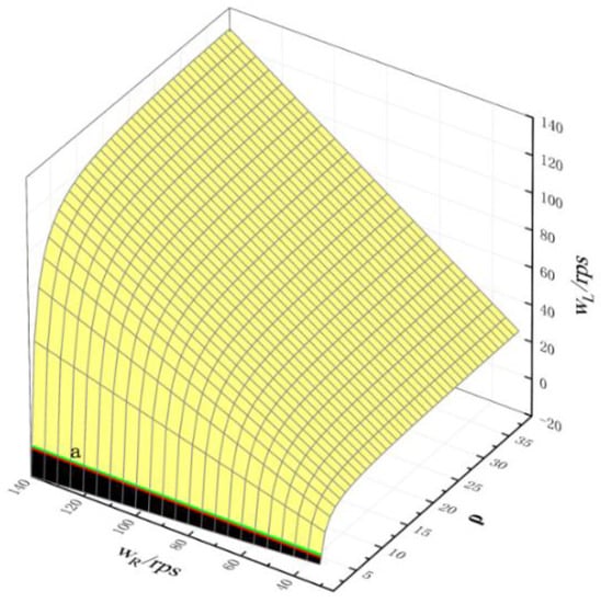
Figure 5.
The corresponding relationship between , and under cement pavement.
Curve a is the equivalent curve when b = 0, indicating that the implicated velocity of the left track of the robot is 0. Below curve a is a negative value, indicating that the track rotation direction is opposite to the prescribed direction. Above curve a is a positive value, indicating that the track rotation direction is the same as the prescribed direction. As shown in Figure 5, when the tracked robot is in steering motion, the magnitude and direction of the left speed track speed are also different to complete the curve motion with different relative steering radii when the right track speed is fixed. For example, when is small, is negative, which is opposite to the rotation direction of . When gradually increases, changes from negative to positive, which is the same as the rotation direction of .
To clarify the correspondence between , and , the equivalent curves of the three parameters were drawn.
As shown in Figure 6, when the steering radius of the robot is small, , the angular velocity of the left track motor changes rapidly, whereas when the steering radius is large, , the angular velocity of the left track motor changes slightly.
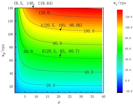
Figure 6.
Motor contour curve under cement road.
Taking points A, B, and C on the contour curve, it can be observed that when the track speeds on both sides are well-controlled, the robot can complete the steering motion with the same steering radius at different speeds. For example, the relative steering radii of A and B are 20.5, but the angular velocities of the tracks on both sides are (105 r/s, 90.06 r/s) and (65 r/s, 60.7 r/s), respectively. When the robot’s track speed was high, the robot could not complete a small steering motion. For example, at point C, the left track speed of the robot was 119.65 r/s, and the right track speed reached the maximum. The minimum relative steering radius that the robot could achieve was 8.5, and its corresponding steering radius was 6.71 m.
5. Obstacle-Avoidance Steering Control Strategy and Simulation Analysis
Robots face many types of obstacles, and the steering control method is generally the same. This study considered angular obstacles as the research object for studying their control characteristics.
5.1. Principle Analysis of Obstacle Avoidance Steering in Right Angular Obstacles
The obstacle-avoidance steering motion of the robot in the face of angular obstacles is illustrated in Figure 7. There are various ways for a robot to choose during the steering process. According to the steering mode, the robot can be divided into center- and small-radius steering motions.
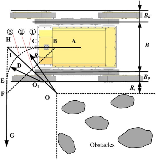
Figure 7.
Principle analysis of robot steering.
The center steering motion is used to complete angular obstacles; the schemes adopted are ABCHEFG and ABFG, as shown in Figure 7, curve ① and ②. The former only needs one center steering movement, while the latter needs two center steering movements to complete. When BH and HF are equal, equilateral center steering occurs; when BH and HF are not equal, non-equilateral center steering occurs, and the sum of the two steering angles is 90°. The robot used the small-radius steering mode to complete the angular obstacles, and the ABCIEFG scheme was adopted, as shown in Figure 7.
During the steering process of the robot, the steering radius can be determined by using the following formula:
where is the distance of the robot from the side obstacles, which is also the safe distance for the robot not to collide with the side obstacles when driving and can be determined according to the size of the driving space. is the distance between the center of the robot’s track and its boundary.
In several steering schemes, the control mode of the robot driving the wheel motor is completely different; for example, the rotation direction and size of the motor are not consistent; therefore, it is necessary to determine the driving parameters of the robot in the face of angular obstacles.
5.2. Simulation Analysis of Obstacle Avoidance Steering Motion
Based on a theoretical analysis of the steering control strategy of the robot’s angular obstacles, it was found that the robot can choose many schemes when facing an angular obstacle. The 3D models of the robot and terrain were established using Solidworks software according to the parameters. The 3D models were converted into X_T format and then imported into ADAMS simulation software. Constraints were added to test models through the simulation software, and motor drive functions were edited to make the robot walk according to the predetermined trajectory. The robot’s driving road has no mutation, and friction coefficients between robot’s track and road were the same. Finally, the corresponding simulation test was completed.
In the process of obstacle avoidance and steering, the robot implemented the necessary acceleration and deceleration motions and maintained full speed at other times. The maximum inspection speed of the robot was set at 550 m/s. The steering velocity curve of the tracked robot and angular velocity of the track wheel are shown in Figure 8, where Angular_v_R is the angular velocity of the right track, Angular_v_L is the angular velocity of the left track; V is the actual velocity of the robot, and V’ is the theoretical velocity of the robot (regardless of the skid and slip). The skid or slip rate of right track is defined as iR, and iL is the skid or slip rate of left track; the numbers ①, ②, and ③ are the steering movement of the robot in the three schemes. It can be seen that all tracked robots can complete obstacle-avoidance steering as required; however, they have their own characteristics.
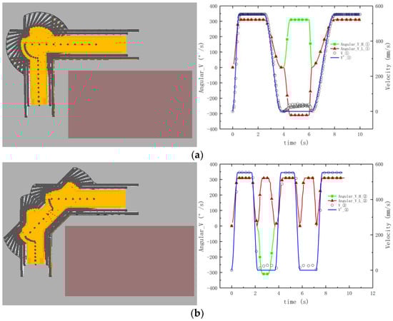
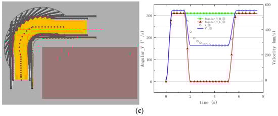
Figure 8.
Angular obstacle-avoidance steering simulation. (a) Obstacle-avoidance steering motion shown in scheme 1 (10.2 s); (b) Obstacle-avoidance steering motion shown in scheme 2 (9.4 s); (c) Obstacle-avoidance steering motion shown in scheme 3 (7.5 s).
The robot completes the obstacle steering movement through scheme 1, which requires three rounds of steering and speed switching of the track’s drive motor on both sides. This scheme is easy to control; however, the steering time is long, requiring 10.2 s, and the required space for steering is large. When the robot was in a narrow space, it was not conducive to steering. The robot can complete the angular obstacle steering movement through scheme 2, which is simple to operate and requires 9.4 s, less time than scheme 1, but it needs to switch the steering and speed of the two motors five times. In this steering scheme, the robot is prone to collision at the corner point; therefore, special attention should be paid to controlling the corner points. The robot can complete the angular obstacle steering movement through scheme 3, which only needs to switch the steering and speed of the right motor once, which takes 7.5 s. This steering scheme requires a small space range and has good stationarity; however, the skid and slip rates are high in the steering process. Therefore, it is necessary to fully grasp the driving and road characteristics of the tracked robot and provide accurate motor driving parameters to realize it.
The skid and slip rate of the tracked robot through three strategies are shown in Figure 9. The part above the zero-axis is the slip rate, and the part below the zero-axis is the skid rate. From the figure, it can be seen that skid and slip will be shown at different stages of the robot’s steering. At the moment when the robot starts, the robot slips, which decreases with the increase of the robot’s speed, as shown in point A in the three figures. The slip rate of the tracked robot is small when robot drive in a straight line, as shown in point B. The tracked robot has a large skid rate at the moment of deceleration, and the whole body moves forward under the action of inertia, as shown in point C. The tracked robot has a larger slip rate when turning in situ center, and the slip rate of the low-speed track (0.39) is greater than that of the high-speed track (0.35), the slip rate of the tracked robot through arc steering is small, 0.27 in scheme 3, as shown in point D. The relevant data of the tracked robot is shown in Table 3.
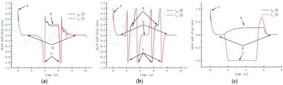
Figure 9.
Skid and slip rate. (a) scheme 1; (b) scheme 2; (c) scheme 3.
Table 3.
Related data comparison table of the tracked robot.
5.3. Test and Analysis of Robot Obstacle-Avoidance Steering
In this experiment, the obstacles were set manually. The obstacle-avoidance steering process of the robot is shown in Figure 10a. It can be observed from the figure that the tracked robot completed the obstacle-avoidance steering motion according to the three schemes.
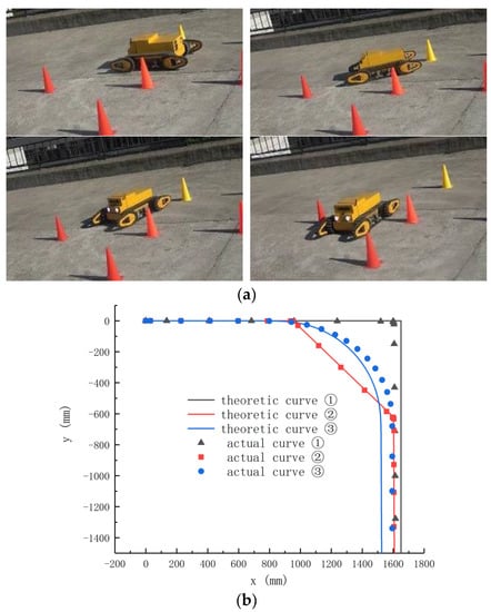
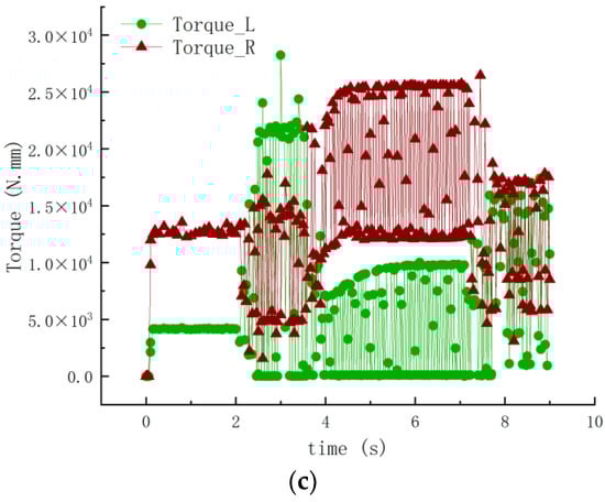
Figure 10.
Robot obstacle-avoidance steering performance test. (a) Robot obstacle-avoidance steering test process. (b) Robot obstacle-avoidance steering trajectory. (c) Tracked wheel motor torque in scheme 3.
The steering trajectory of the robot is shown in Figure 10b, where “theoretical curve” are the theoretical curves, which considers the influence of skid and slip on its steering performance, and “actual curve” are the actual curves, which do not consider the influence of sliding on steering performance. Curves ①, ② and ③ are the obstacle-avoidance steering experiments completed by three schemes, respectively. It can be seen from Figure 9b that in the trajectory of the robot, in the initial stage, there is no error when the robot drives along a straight line in the three steering modes, but after steering, the X-coordinates of the end points are 1623 mm, 1606 mm and 1595 mm respectively, while the predetermined value is 1650 mm; however, the difference has little influence on overall steering. In particular, when the robot turns in the third scheme, the theoretical steering radius of the robot is R = 395 mm according to the speed difference between the track wheels on both sides of the robot, and the actual steering radius of the robot is R = 634 mm under the influence of track skid and slip, with a difference of 239 mm and a large deviation. Therefore, the track structure and road conditions of the robot should be considered for the accurate control of the autonomous obstacle-avoidance steering of the robot.
It can be seen from Figure 10c that the steering process of the robot is from 4 to 7.8 s, and the traction force of the right track wheel of the robot is significantly larger than that of the left track wheel, with a maximum traction force of 25 KN·m, whereas the traction forces of the two track wheels were roughly the same at other times.
From the above analysis, it can be seen that the robot can complete the obstacle-avoidance steering motion in three ways, which indicates that the steering control strategy is correct, and that the control strategy can provide the corresponding theoretical basis for autonomous obstacle-avoidance navigation control of the robot. The robot adopts large-radius obstacle-avoidance steering motion control, which has a smooth trajectory, fast steering speed, and the highest efficiency. However, the skid and slip of the track have a great influence on this control method; therefore, the robot driving speed, road characteristics, and other relevant information is needed, which leads to the increasing difficulty of robot control that is not easy to master.
6. Conclusions
In this paper, the theory of obstacle-avoidance steering control strategies can be applied to tracked robots in general, and precise trajectory-tracking control of tracked robots can be realized under the influence of skids and slips.
(1) The steering radius of the tracked robot was analyzed according to its structural characteristics, the load analysis of the unit track length of the robot was completed and the expressions of the tractive force and steering resistance of the robot were established. Through the analysis and simulation of the steering plane dynamics of the robot, the corresponding relationships among the track structure, the relative steering radius and ground parameters were obtained under several typical road conditions.
(2) The relationship between the driving parameters of the motor and the relative steering radius of the robot under skid and slip conditions were constructed. The corresponding relationship between the relative steering radius of the robot and the rotation speed and direction of the tracks on both sides of the robot were obtained by simulation analysis. The slip rate of the tracked robot is small when robot drive in a straight line. The tracked robot has a larger slip rate when turning in situ center, and the slip rate of the low-speed track (0.39) is greater than that of the high-speed track (0.35). The slip rate of the tracked robot using arc steering is small, and its slip rate is 0.27.
(3) The steering control strategies of once turning in situ center, twice turning in situ center and large-radius steering were formulated to complete the obstacle-avoidance steering experiment. The trajectory of the robot using large-radius obstacle-avoidance steering motion was smooth, the steering speed was fast, and the efficiency was the highest. However, under large-radius steering, the skid and slip of the track had a great influence on the steering, the theoretical steering radius of the robot was R = 395 mm, and the actual steering radius was R = 634 mm. Therefore, more precise information is needed through scheme 3, such as the driving speed of the robot and road parameters. Using simulation analysis, the robot prototype completed the obstacle-avoidance steering experiment, which verifies the rationality of the robot skid-steering theory.
This paper proposed that obstacle-avoidance steering control strategies can be applied to tracked devices in general, where the occurrence of skid and slip cannot be disregarded. This paper could provide a reference for autonomous obstacle-avoidance navigation control of tracked robots. But there are still some areas for improvement in this paper; in order to realize the steering control of robot obstacle-avoidance, it is necessary to build a control system including multi-sensor information fusion to detect road parameters in real time.
Author Contributions
Conceptualization, C.W., H.M. and L.Z.; methodology, X.X. and H.T.; writing—original draft preparation, S.W. and H.Z.; writing—review and editing, C.W.; project administration, C.W. and L.Z. All authors have read and agreed to the published version of the manuscript.
Funding
This work was supported in part by the National Natural Science Foundation of China under Grant 51975468, in part by the Shaanxi Provincial Department of Education to Serve Local Special Program Projects under Grant 22JC051, in part by the Key Laboratory of Road Construction Technology and Equipment under Grant 300102259508.
Institutional Review Board Statement
Not applicable.
Informed Consent Statement
Not applicable.
Data Availability Statement
The data presented in this study are available on request from the first author.
Conflicts of Interest
The authors declare no conflict of interest.
References
- Ding, Z.; Wang, Z.; Su, Z.; Tian, L.; Xiong, Y.; Wu, X.; Tang, Z. A New Model to Predict the Slippage Coefficient of Tracked Vehicles During Steering. IEEE Access 2022, 10, 72006–72014. [Google Scholar] [CrossRef]
- Boschetti, G.; Bottin, M.; Faccio, M.; Maretto, L.; Minto, R. The influence of collision avoidance strategies on human-robot collaborative systems. Ifac-Papersonline 2022, 55, 301–306. [Google Scholar] [CrossRef]
- Scoccia, C.; Palmieri, G.; Palpacelli, M.C.; Callegari, M. Real-Time Strategy for Obstacle Avoidance in Redundant Manipulators. In Advances in Italian Mechanism Science; Mechanisms and Machine Science Book Series; Springer: Berlin, Germany, 2020; pp. 278–285. [Google Scholar]
- Faccio, M.; Minto, R.; Rosati, G.; Bottin, M. The influence of the product characteristics on human-robot collaboration: A model for the performance of collaborative robotic assembly. Int. J. Adv. Manuf. Technol. 2019, 106, 2317–2331. [Google Scholar] [CrossRef]
- Gonon, D.J.; Paez-Granados, D.; Billard, A. Robots’ Motion Planning in Human Crowds by Acceleration Obstacles. IEEE Robot. Autom. Lett. 2022, 7, 11236–11243. [Google Scholar] [CrossRef]
- Murtaza, M.A.; Aguilera, S.; Waqas, M.; Hutchinson, S. Safety Compliant Control for Robotic Manipulator With Task and Input Constraints. IEEE Robot. Autom. Lett. 2022, 7, 10659–10664. [Google Scholar] [CrossRef]
- Frank, F.; Paraschos, A.; van der Smagt, P.; Cseke, B. Constrained Probabilistic Movement Primitives for Robot Trajectory Adaptation. IEEE Trans. Robot. 2022, 38, 1–2. [Google Scholar] [CrossRef]
- Dai, Y.; Xiang, C.; Zhang, Y.; Jiang, Y.; Qu, W.; Zhang, Q. A Review of Spatial Robotic Arm Trajectory Planning. Aerospace 2022, 9, 361. [Google Scholar] [CrossRef]
- Kitano, M.; Jyozaki, H. A theoretical analysis of steerability of tracked vehicles. J. Terramechanics 1976, 13, 241–258. [Google Scholar] [CrossRef]
- Wong, J.Y.; Chiang, C.F. A general theory for skid steering of tracked vehicles on firm ground. Proc. Inst. Mech. Eng. Part D J. Automob. Eng. 2001, 215, 343–355. [Google Scholar] [CrossRef]
- Dong, C.; Cheng, K.; Hu, W.; Yao, Y.; Gao, X. Kinematic and dynamic modeling of all terrain articulated tracked vehicle in process of spin steering. J. Cent. South Univ. Sci. Technol. 2017, 48, 1481–1491. [Google Scholar]
- Gai, J.T.; Liu, C.S.; Ma, C.J.; Shen, H.J. Steering control of electric drive tracked vehicle considering tracks’ skid and slip. Acta Armamentarii 2021, 42, 2092–2101. [Google Scholar]
- Gao, Q.; Pan, D.; Zhang, X.; Deng, F.; Huang, D.; Wang, L. Design and simulation of entire track modular unmanned agricultural power chassis. Trans. Chin. Soc. Agric. Mach. 2020, 51, 561–570. [Google Scholar]
- Guan, Z.H.; Mu, S.L.; Wu, C.Y.; Chen, K.Y.; Liao, Y.T.; Ding, Y.C.; Liao, Q.X. Steering kinematic analysis and experiment of tracked combine harvester working in paddy field. Trans. Chin. Soc. Agric. Eng. 2020, 36, 29–38. [Google Scholar]
- Dai, Y.; Zhang, J.; Zhang, T.; Liu, S.J. Motion simulation of the deep ocean mining system based on its integrated multi-body dynamic model. J. Mech. Eng. 2017, 53, 155–160. [Google Scholar] [CrossRef]
- Han, Z.H.; Zhu, L.C.; Yuan, Y.W.; Zhao, B.; Fang, X.F.; Zhang, T.F. Analysis of slope trafficability and optimized design of crawler chassis in hillside orchard. Trans. Chin. Soc. Agric. Mach. 2022, 53, 413–421+448. [Google Scholar]
- Zou, T.; Angeles, J.; Hassani, F. Dynamic Modeling and Trajectory Tracking Control of Unmanned Tracked Vehicles. Robot. Auton. Syst. 2018, 110, 102–111. [Google Scholar] [CrossRef]
- Ding, Z.; Li, Y.; Tang, Z. Theoretical Model for Prediction of Turning Resistance of Tracked Vehicle on Soft Terrain. Math. Probl. Eng. 2020, 2020, 4247904. [Google Scholar] [CrossRef]
- Kuwahara, H.; Murakami, T. Position Control Considering Slip Motion of Tracked Vehicle Using Driving Force Distribution and Lateral Disturbance Suppression. IEEE Access 2022, 10, 20571–20580. [Google Scholar] [CrossRef]
- Wang, C.; Ma, K.; Yang, L.; Ma, H.; Xue, X.; Tian, H. Simulation and experiment on obstacle-surmounting performance of four swing arms and six tracked robot under unilateral step environment. Trans. Chin. Soc. Agric. Eng. 2018, 34, 46–53. [Google Scholar]
- Strawa, N.; Ignatyev, D.I.; Zolotas, A.C.; Tsourdos, A. On-Line Learning and Updating Unmanned Tracked Vehicle Dynamics. Electronics 2021, 10, 187. [Google Scholar] [CrossRef]
- Prado, A.J.; Torres-Torriti, M.; Cheein, F.A.A. Distributed Tube-Based Nonlinear MPC for Motion Control of Skid-Steer Robots with Terra-Mechanical Constraints. IEEE Robot. Autom. Lett. 2021, 6, 8045–8052. [Google Scholar] [CrossRef]
- Wong, J. Optimization of the Tractive Performance of Articulated Tracked Vehicles Using an Advanced Computer Simulation Model. Proceedings of the Institution of Mechanical Engineers, Part D: Journal of Automobile Engineering. 1992, 206, 29–45. [Google Scholar] [CrossRef]
Publisher’s Note: MDPI stays neutral with regard to jurisdictional claims in published maps and institutional affiliations. |
© 2022 by the authors. Licensee MDPI, Basel, Switzerland. This article is an open access article distributed under the terms and conditions of the Creative Commons Attribution (CC BY) license (https://creativecommons.org/licenses/by/4.0/).