

A Reinforcement Learning Model of Multiple UAVs for Transporting Emergency Relief Supplies


Abstract
1. Introduction
- In the UAVRPs, equity metric was implemented to take into account the post-disaster HL situation, demonstrating that the disparity in supplies per evacuation center can be eliminated;
- We proposed a QL algorithm for solving UAVRPs, discussed the parameter settings of QL, and outperformed meta-heuristics methods in the conditions of the previous study;
- We introduced three metrics that are considered important in the transportation of supplies in a post-disaster HL. We tested several transport strategies with different weights of the three metrics and evaluated the response of each strategy to each metric.
2. Related Works
2.1. Potential of Using UAVs in Disaster Response
2.2. UAV Routing Problem for Logistics
3. Model Description
3.1. Problem Definition
3.2. Environment
3.3. Agent
- All UAVs are homogeneous; thus, they have the same maximum payload C and maximum amount of energy E;
- At the start of the transport, all UAVs are assumed to be at the depot;
- The batteries are fully charged when the UAV takes off from the depot;
- Since there are sufficient batteries for the UAV in the depot, the battery charging time is not considered;
- Each UAV has its batteries replaced only at the depot.
3.4. Cost Functions
- Flight Time Cost (): The cost based on the total flight time of all UAVs. This corresponds to rapidity;
- Priority Cost (): The cost based on quick transportation of high-priority supplies. This corresponds to urgency;
- Equity Cost (): The cost based on equitable transportation to all shelters. This corresponds to equity.
4. Proposed Method
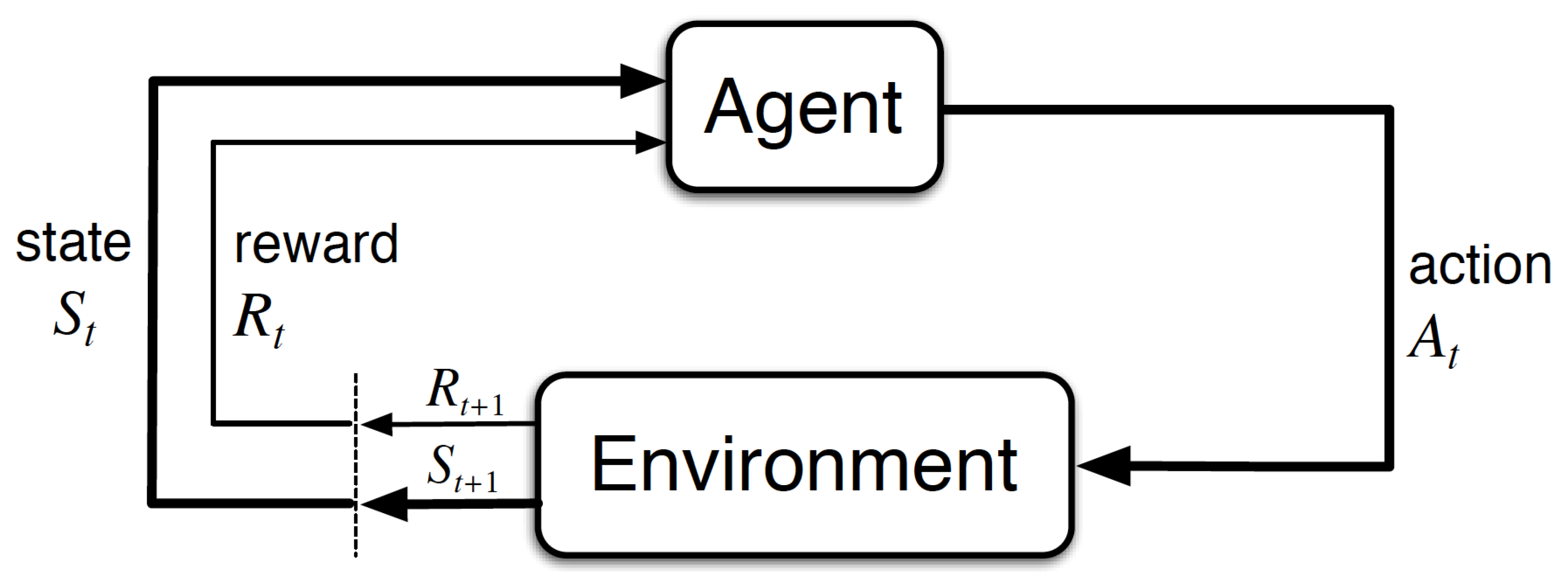
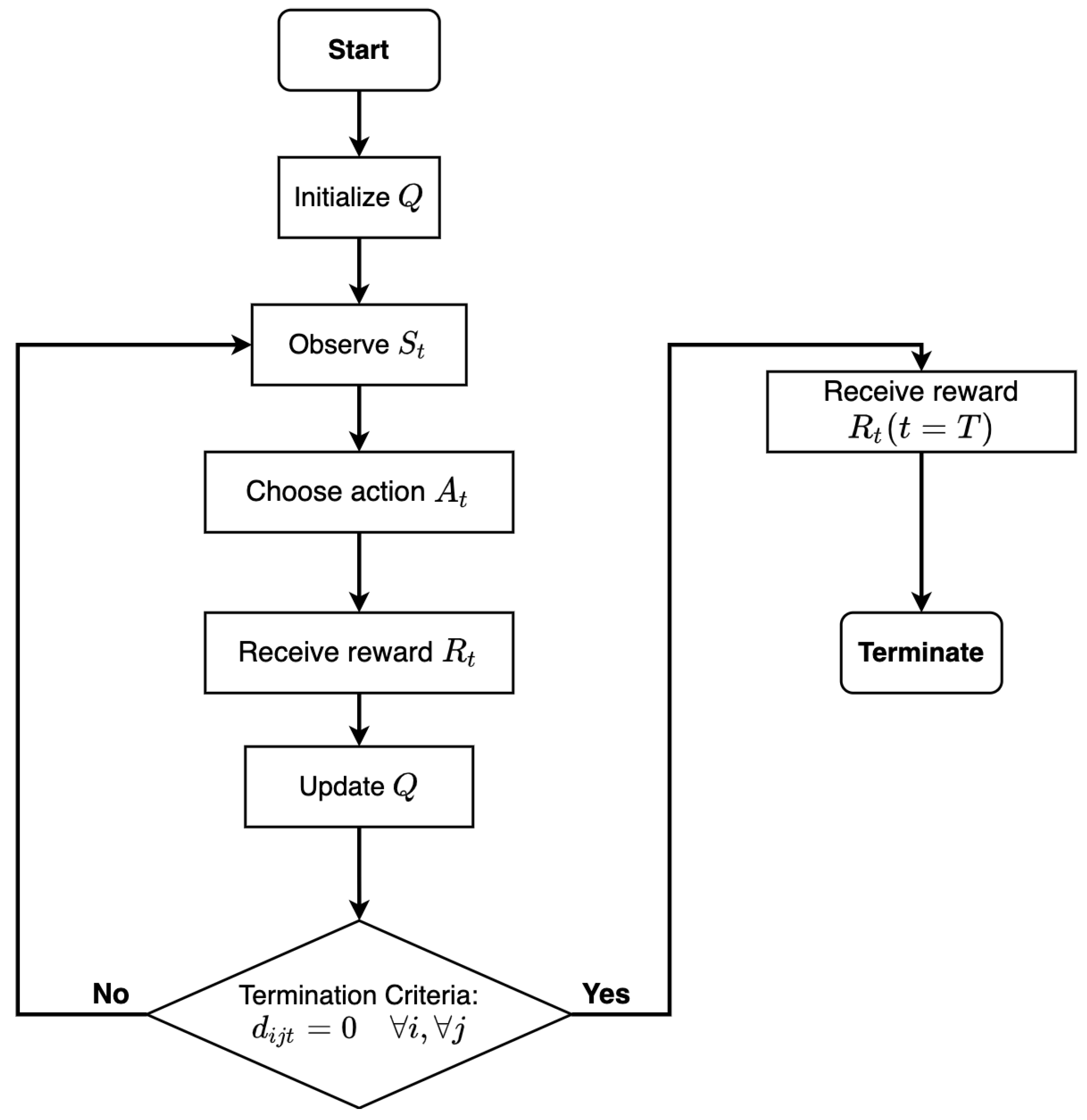
4.1. Q-Learning
4.2. State and Action
- States: A state at instant t, , represents the set of the remaining shelter demand at instant t. is denoted by , where is the set of demands of shelter j at instant t.
- Actions: Selection of the following two elements among all possible actions: (i) the shelter/depot to transport/return and (ii) the amount of items that the UAV transports. Note that the types of supplies are selected in order of urgency among the supplies demanded by the destination shelter. An action at instant t, , is denoted by .
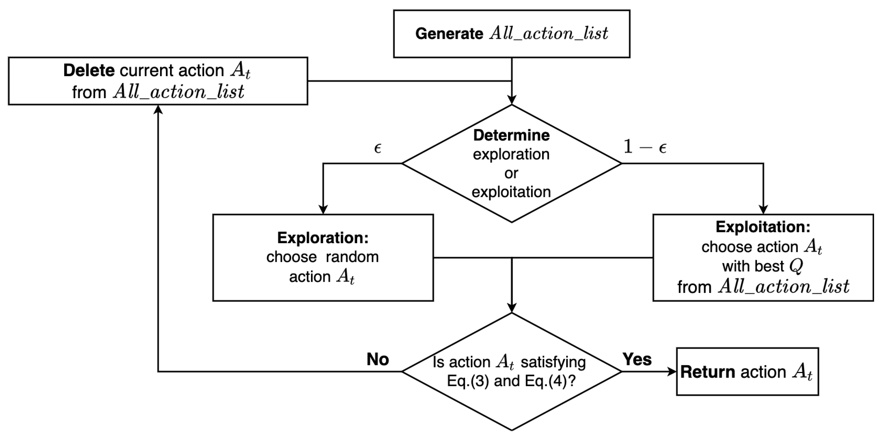
4.3. Policy
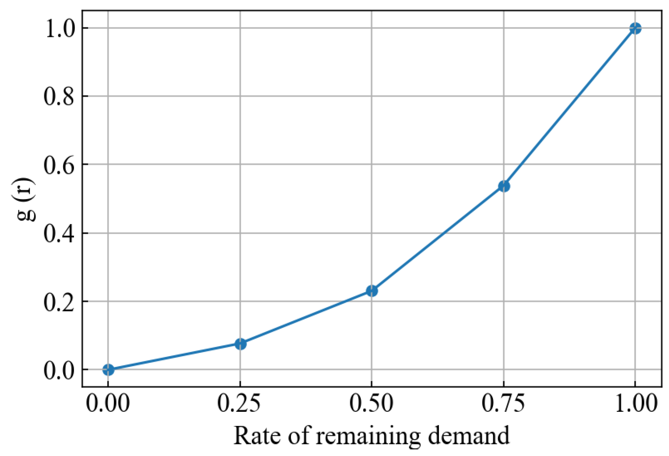
4.4. Reward
5. Numerical Experiments
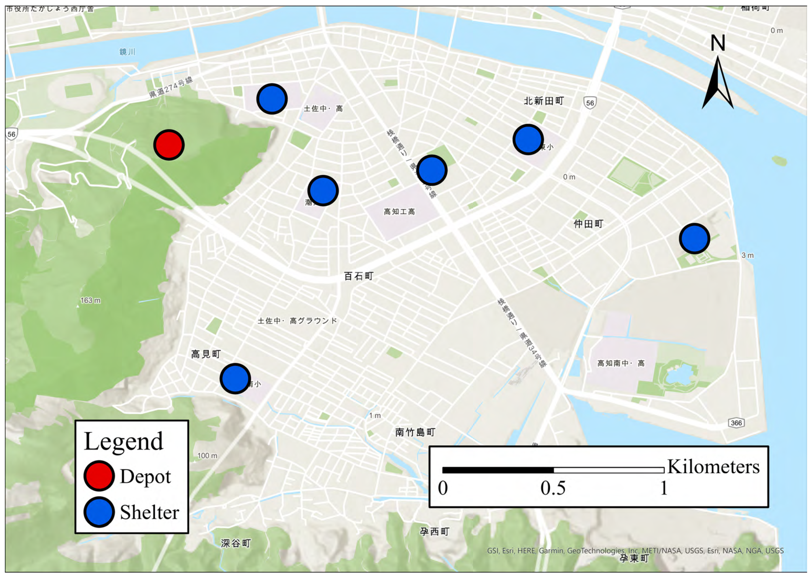
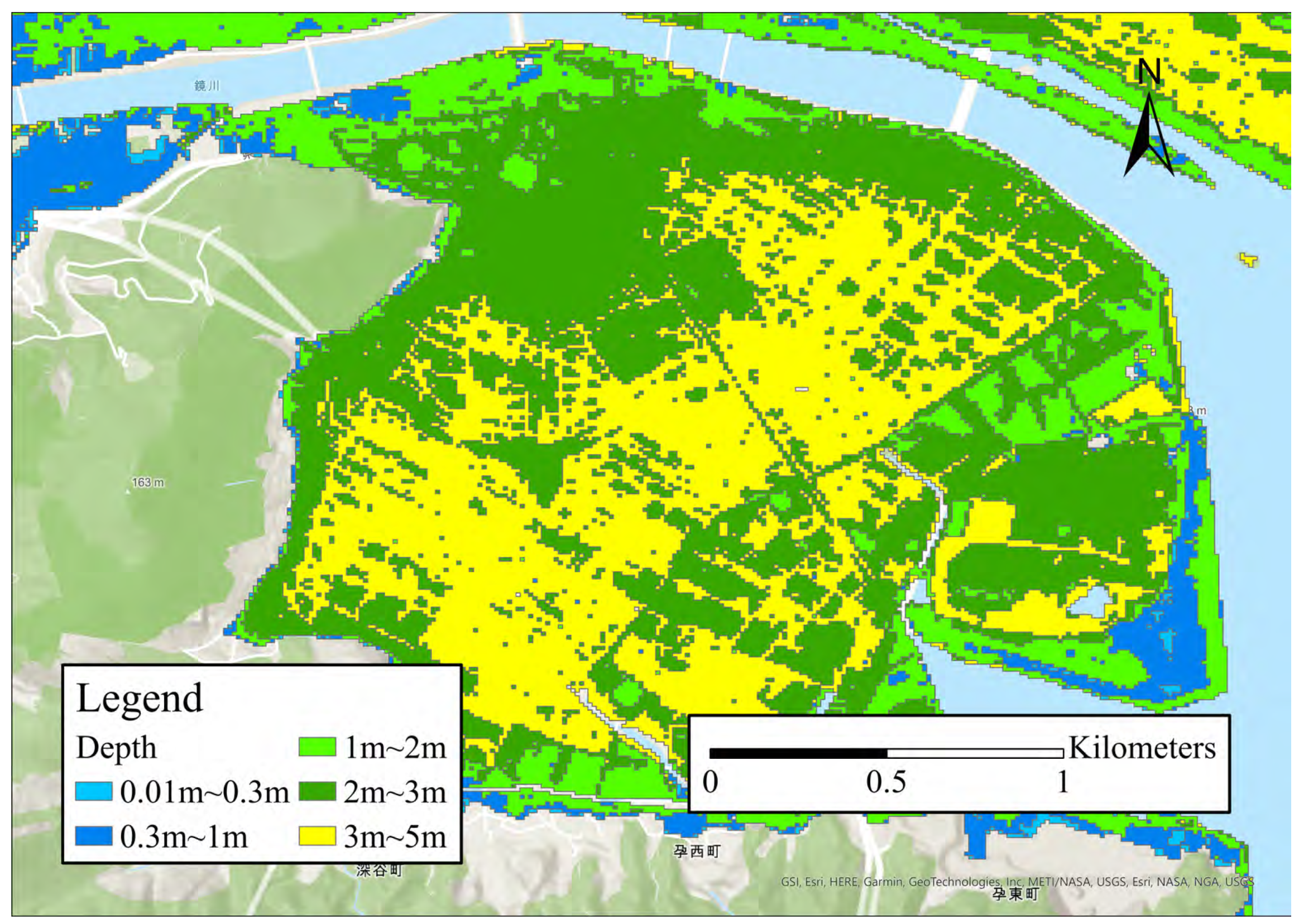
5.1. Simulation Settings
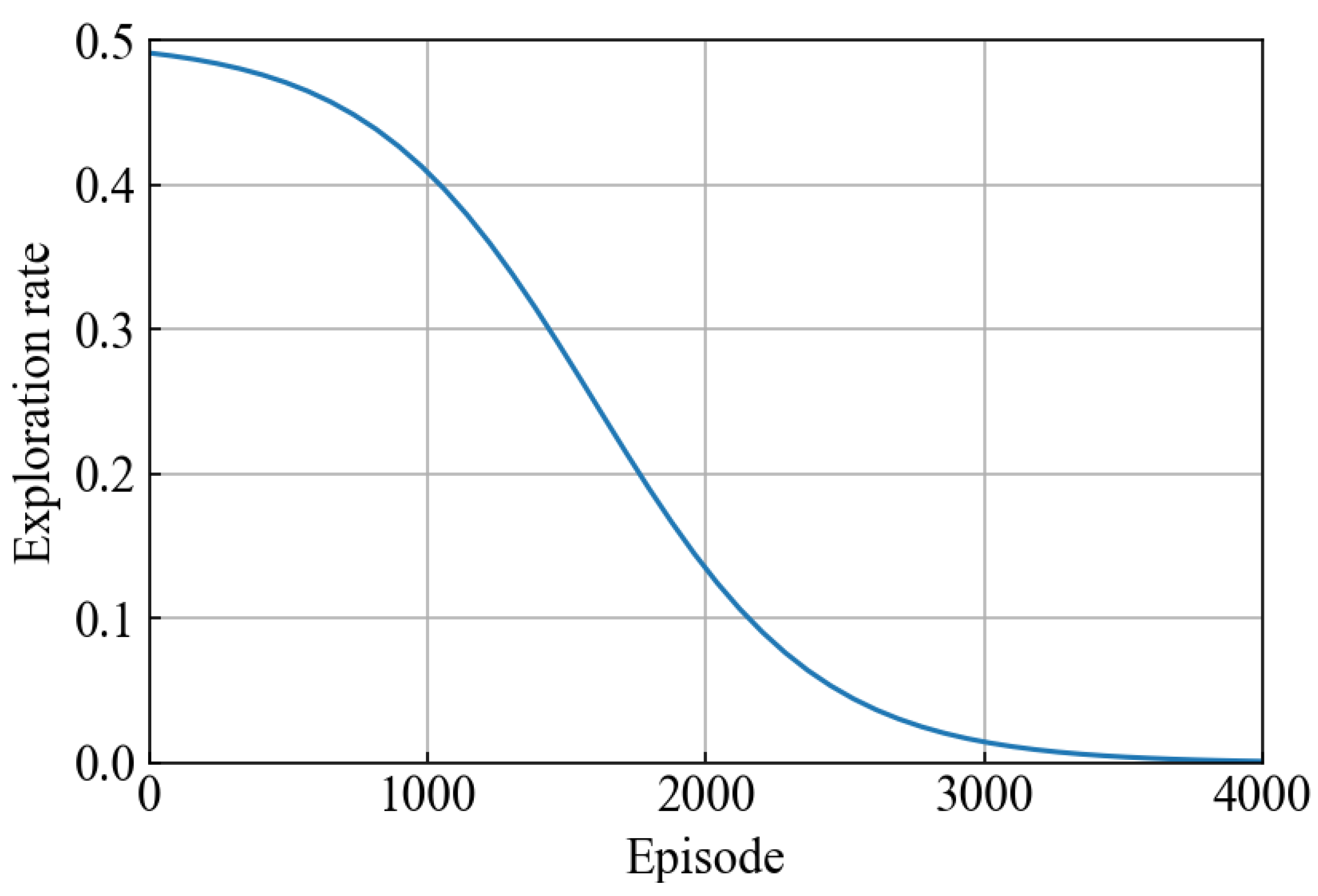
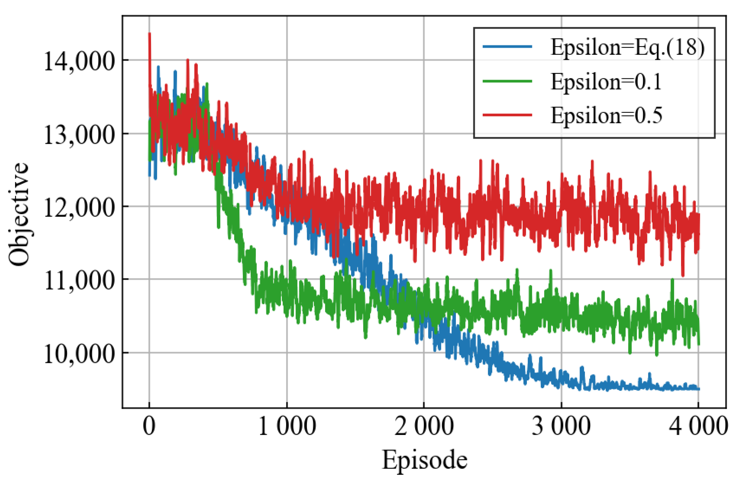
5.2. Parameter Settings
5.3. Comparison of Methods
- Maximum payload of UAV;
- Time window for transportation at each point.
5.4. Performance Comparison
6. Conclusions and Future Work
Author Contributions
Funding
Institutional Review Board Statement
Informed Consent Statement
Data Availability Statement
Conflicts of Interest
References
- Balcik, B.; Beamon, B.; Smilowitz, K. Last mile distribution in humanitarian relief. J. Intell. Transp. Syst. 2008, 12, 51–63. [Google Scholar] [CrossRef]
- Dubey, R.; Luo, Z.; Gunasekaran, A.; Akter, S.; Hazen, B.T.; Douglas, M.A. Big data and predictive analytics in humanitarian supply chains. Int. J. Logist. Manag. 2018, 29, 485–512. [Google Scholar] [CrossRef]
- Suzuki, Y. Impact of material convergence on last-mile distribution in humanitarian logistics. Int. J. Prod. Econ. 2020, 223, 107515. [Google Scholar] [CrossRef]
- Jaller, M. Resource Allocation Problems during Disasters: The Cases of Points of Distribution Planning and Material Convergence Handling; Rensselaer Polytechnic Institute: Troy, NY, USA, 2011. [Google Scholar]
- Das, R. Disaster preparedness for better response: Logistics perspectives. Int. J. Disaster Risk Reduct. 2018, 31, 153–159. [Google Scholar] [CrossRef]
- Holgun-Veras, J.; Taniguchi, E.; Jaller, M.; Aros-Vera, F.; Ferreira, F.; Thompson, R.G. The Tohoku disasters: Chief lessons concerning the post disaster humanitarian logistics response and policy implications. Transp. Res. Part A Policy Pract. 2014, 69, 86–104. [Google Scholar] [CrossRef]
- Shibata, Y.; Uchida, N.; Shiratori, N. Analysis of and proposal for a disaster information network from experience of the Great East Japan Earthquake. IEEE Commun. Mag. 2014, 52, 44–50. [Google Scholar] [CrossRef]
- Sato, T.; Suzuki, K. Impact of Transportation Network Disruptions caused by the Great East Japan Earthquake on Distribution of Goods and Regional Economy. J. JSCE 2013, 1, 507–515. [Google Scholar] [CrossRef]
- Koshimura, S.; Hayashi, S.; Gokon, H. The impact of the 2011 Tohoku earthquake tsunami disaster and implications to the reconstruction. Soils. Found. 2014, 54, 560–572. [Google Scholar] [CrossRef]
- Nakachi, H.; Maki, N.; Hayashi, H.; Kobayashi, K. A Proposal of the Effective System to Utilize Helicopt ers During the Giant Earthquake Disaster of the Nankai Trough Based on the Study of the Great East Japan Earthquake. J. JSNDS 2014, 33, 101–114. (In Japanese) [Google Scholar]
- Kellermann, R.; Fisher, L. Drones for parcel and passenger transportation: A literature review. Transport. Res. Interdiscip. Persp. 2020, 4, 100088. [Google Scholar] [CrossRef]
- Al-Turjman, F.; Alturjman, S. 5G/IoT-enabled UAVs for multimedia delivery in industry-oriented applications. Multimed. Tools. Appl. 2020, 79, 8627–8648. [Google Scholar] [CrossRef]
- Cheng, C.; Adulyasak, Y.; Rousseau, L.M. Drone routing with energy function: Formulation and exact algorithm. Transp. Res. Part B Methodol. 2020, 139, 364–387. [Google Scholar] [CrossRef]
- Yakushiji, K.; Fujita, H.; Murata, M.; Hiroi, N.; Hamabe, Y.; Yakushiji, F. Short-Range Transportation Using Unmanned Aerial Vehicles (UAVs) during Disasters in Japan. Drones 2020, 4, 68. [Google Scholar] [CrossRef]
- Magdalena, P.; Lora, K. Zipline’s New Drone Can Deliver Medical Supplies at 79 Miles per Hour. CNBS. Available online: Https://www.cnbc.com/2018/04/02/zipline-new-zip-2-drone-delivers-supplies-at-79-mph.html (accessed on 14 September 2022).
- Thibbotuwawa, A.; Bocewicz, G.; Nielsen, P.; Banaszak, Z. Unmanned Aerial Vehicle Routing Problems: A Literature Review. Appl. Sci. 2020, 10, 4504. [Google Scholar] [CrossRef]
- Dorling, K.; Heinrichs, J.; Messier, G.G.; Magierowski, S. Vehicle Routing Problems for Drone Delivery. IEEE Trans. Syst. Man Cybern. Syst. 2017, 47, 70–85. [Google Scholar] [CrossRef]
- Rabta, B.; Wankmüller, C.; Reiner, G. A drone fleet model for last-mile distribution in disaster relief operations. Int. J. Disaster Risk Reduct. 2018, 28, 107–112. [Google Scholar] [CrossRef]
- Shi, Y.; Lin, Y.; Li, B.; Yi Man Li, R. A bi-objective optimization model for the medical supplies’ simultaneous pickup and delivery with drones. Comput. Ind. Eng. 2022, 171, 108389. [Google Scholar] [CrossRef]
- Ghelichi, Z.; Gentili, M.; Mirchandani, P.B. Logistics for a fleet of drones for medical item delivery: A case study for Louisville, KY. Comput. Oper. Res. 2021, 135, 105443. [Google Scholar] [CrossRef]
- Jiang, X.; Zhou, Q.; Ye, Y. Method of Task Assignment for UAV Based on Particle Swarm Optimizationin logistics. In Proceedings of the 2017 International Conference on Intelligent Systems, Metaheuristics & Swarm Intelligence, Hong Kong, China, 25–27 March 2017; pp. 113–117. [Google Scholar]
- Song, B.D. Persistent UAV delivery logistics: MILP formulation and efficient heuristic. Comput. Ind. Eng. 2018, 120, 418–428. [Google Scholar] [CrossRef]
- Li, Y.; Yuan, X.; Zhu, J.; Huang, H.; Wu, M. Multiobjective Scheduling of Logistics UAVs Based on Variable Neighborhood Search. Appl. Sci. 2020, 10, 3575. [Google Scholar] [CrossRef]
- Gentili, M.; Mirchandani, P.B.; Agnetis, A.; Ghelichi, Z. Locating Platforms and Scheduling a Fleet of Drones for Emergency Delivery of Perishable Items. Comput. Ind. Eng. 2022, 168, 108057. [Google Scholar] [CrossRef]
- Chowdhury, S.; Emelogu, A.; Marufuzzaman, M.; Nurre, S.G.; Bian, L. Drones for disaster response and relief operations: A continuous approximation model. Int. J. Prod. Econ. 2017, 188, 167–184. [Google Scholar] [CrossRef]
- Chen, J.; Du, C.; Zhang, Y.; Han, P.; Wei, W. A Clustering-Based Coverage Path Planning Method for Autonomous Heterogeneous UAVs. IEEE Trans. Intell. Transp. Syst. 2021, 1–11. [Google Scholar] [CrossRef]
- Chen, J.; Ling, F.; Zhang, Y.; You, T.; Liu, Y.; Du, X. Coverage path planning of heterogeneous unmanned aerial vehicles based on ant colony system. Swarm Evol. Comput. 2022, 69, 101005. [Google Scholar] [CrossRef]
- Beamon, B.M.; Balcik, B. Performance measurement in humanitarian relief chains. Int. J. Public Sect. Manag. 2008, 21, 4–25. [Google Scholar] [CrossRef]
- Huang, M.; Smilowitz, K.; Balcik, B. Models for relief routing: Equity, efficiency and efficacy. Transp. Res. Part E Logist. Transp. Rev. 2012, 48, 2–18. [Google Scholar] [CrossRef]
- Watkins, C.J.; Dayan, P. Q-learning. Mach. Learn. 1992, 8, 279–292. [Google Scholar] [CrossRef]
- Sakurai, M.; Murayama, Y. Information technologies and disaster management-Benefits and issues-. Prog. Disaster Sci. 2019, 2, 100012. [Google Scholar] [CrossRef]
- Yu, M.; Yang, C.; Li, Y. Big Data in Natural Disaster Management: A Review. Geosciences 2018, 8, 165. [Google Scholar] [CrossRef]
- Zacharie, M.; Fuji, S.; Minori, S. Rapid Human Body Detection in Disaster Sites Using Image Processing from Unmanned Aerial Vehicle (UAV) Cameras. In Proceedings of the 2018 International Conference on Intelligent Informatics and Biomedical Sciences (ICIIBMS), Bangkok, Thailand, 21–24 October 2018. [Google Scholar]
- Nagasawa, R.; Mas, E.; Moya, L.; Koshimura, S. Model-based analysis of multi-UAV path planning for surveying postdisaster building damage. Sci. Rep. 2021, 11, 18588. [Google Scholar] [CrossRef]
- Alhindi, A.; Alyami, D.; Alsubki, A.; Almousa, R.; Al Nabhan, N.; Al Islam, A.B.M.A.; Kurdi, H. Emergency Planning for UAV-Controlled Crowd Evacuations. Appl. Sci. 2021, 11, 9009. [Google Scholar] [CrossRef]
- Klaine, P.V.; Nadas, J.P.B.; Souza, R.D.; Imran, M.A. Distributed Drone Base Station Positioning for Emergency Cellular Networks Using Reinforcement Learning. Cogn. Comput. 2018, 10, 790–804. [Google Scholar] [CrossRef] [PubMed]
- Chowdhury, S.; Shahvari, O.; Marufuzzaman, M.; Li, X.; Bian, L. Drone routing and optimization for post-disaster inspection. Comput. Ind. Eng. 2021, 159, 107495. [Google Scholar] [CrossRef]
- Tiwari, A.; Dixit, A. Unmanned aerial vehicle and geospatial technology pushing the limits of development. Am. J. Eng. Res. 2015, 4, 16–21. [Google Scholar]
- Murray, C.C.; Chu, A.G. The flying sidekick traveling salesman problem: Optimization of drone-assisted parcel delivery. Trans. Res. Emerg. Technol. 2015, 54, 86–109. [Google Scholar] [CrossRef]
- Jeong, H.Y.; Song, B.D.; Lee, S. Truck-drone hybrid delivery routing: Payload-energy dependency and No-Fly zones. Int. J. Prod. Econ. 2019, 214, 220–233. [Google Scholar] [CrossRef]
- Kuo, R.; Lu, S.-H.; Lai, P.-Y.; Mara, S.T.W. Vehicle routing problem with drones considering time windows. Expert Syst. Appl. 2022, 191, 116264. [Google Scholar] [CrossRef]
- Gu, Q.; Fan, T.; Pan, F.; Zhang, C. A vehicle-UAV operation scheme for instant delivery. Comput. Ind. Eng. 2020, 149, 106809. [Google Scholar] [CrossRef]
- Braekers, K.; Ramaekers, K.; Van Nieuwenhuyse, I. The vehicle routing problem: State of the art classification and review. Comput. Ind. Eng. 2016, 99, 300–313. [Google Scholar] [CrossRef]
- Gutjahr, W.J.; Fischer, S. Equity and deprivation costs in humanitarian logistics. Eur. J. Oper. Res. 2018, 270, 185–197. [Google Scholar] [CrossRef]
- Jiang, Z.B.; Gu, J.J.; Fan, W.; Liu, W.; Zhu, B.Q. Q-learning approach to coordinated optimization of passenger inflow control with train skip-stopping on an urban rail transit line. Comput. Ind. Eng. 2019, 127, 1131–1142. [Google Scholar] [CrossRef]
- Yu, L.; Zhang, C.; Jiang, J.; Yang, H.; Shang, H. Reinforcement learning approach for resource allocation in humanitarian logistics. Expert Syst. Appl. 2021, 173, 114663. [Google Scholar] [CrossRef]
- Ministry of Land, Infrastructure, Transport and Tourism of Japan. National Land Numerical Information. Available online: Https://nlftp.mlit.go.jp/ksj/index.html (accessed on 8 June 2022).
- Sheu, J.B. An emergency logistics distribution approach for quick response to urgent relief demand in disasters. Transport. Res. E-Log. 2007, 43, 687–709. [Google Scholar] [CrossRef]
- Lin, Y.; Batta, R.; Rogerson, P.; Blatt, A.; Flanigan, M. A logistics model for emergency supply of critical items in the aftermath of a disaster. Socio-Econ. Plann. Sci. 2011, 45, 132–145. [Google Scholar] [CrossRef]
- Sutton, R.; Barto, A. Reinforcement Learning: An Introduction, 2nd ed.; The MIT Press: Cambridge, MA, USA, 2018; pp. 25–42. [Google Scholar]
- Fang, J.; Hou, H.; Bi, Z.M.; Jin, D.; Han, L.; Yang, J.; Dai, S. Data fusion in forecasting medical demands based on spectrum of post-earthquake diseases. J. Ind. Inf. Integr. 2021, 24, 100235. [Google Scholar] [CrossRef]


| Notation | Description |
|---|---|
| Environment | |
| Number of shelters | |
| Indices for shelters | |
| Set of shelters including the depot () | |
| Number of item types | |
| i | Index for item types |
| Set of item types | |
| Demand of the item i of the shelter j at time instant t | |
| Set of demands of the shelter j at instant t | |
| Set of the remaining demand of all shelters at instant t | |
| Distance between shelter j and k | |
| Penalty cost of item i | |
| Time limit of the item i of the shelter j | |
| Agent | |
| Number of UAVs | |
| l | Index for UAVs |
| Set of UAVs | |
| Amount of item i transport from shelter j to k as nth location in the trip m by UAV l | |
| Number of trips of UAV l | |
| m | Index for trip |
| Number of location that UAV l traveled in trip m (include depot) | |
| n | Index for number of location |
| C | Maximum payload of UAV |
| E | Maximum amount of energy |
| a | Acceleration |
| Maximum speed | |
| Take-off time | |
| Landing time | |
| Servicing time | |
| Flight time between shelter j and k | |
| Transportation cost from shelter j to k | |
| v | Amount of UAV payload |
| Energy needed for take-off and landing for an empty UAV [18] | |
| Additional energy amount needed for take-off and landing with an additional item [18] | |
| Energy to fly one distance unit for an empty UAV [18] | |
| Additional energy amount needed to fly one distance unit with one item [18] | |
| Destination shelter of UAV m at instant t | |
| Time when UAV l transport items for shelter j in trip m | |
| Algorithm | |
| t | instant |
| Action at certain instant t | |
| Agent state at certain instant t | |
| Reward at certain instant t | |
| Q | Action-value function |
| Learning rate | |
| Discount factor | |
| Chance of choosing a random action | |
| Number of episodes | |
| T | Termination time |
| Parameter | Scenario 1 | Scenario 2 | Scenario 3 |
|---|---|---|---|
| Number of UAVs | 3 | 3 | 3 |
| Number of item types | 3 | 3 | 3 |
| Initial demand of each shelter | |||
| Priority rate of each item | |||
| Time limit of each item | |||
| Number of episodes | 8000 | 24,000 | 24,000 |
| Parameter | Value |
|---|---|
| 10 m/s | |
| a | 1 |
| C | 5 kg |
| E | 275 kJ |
| 900 J | |
| 300 J/kg | |
| 3 J/m | |
| 1 | |
| 30 s | |
| 30 s | |
| 60 s |
| Parameter | Value | ||
|---|---|---|---|
| GA | PSO | QL | |
| Population number | 40 | 40 | - |
| Iteration | 100 | 100 | 4000 |
| Calculation times | 50 | 50 | 50 |
Publisher’s Note: MDPI stays neutral with regard to jurisdictional claims in published maps and institutional affiliations. |
© 2022 by the authors. Licensee MDPI, Basel, Switzerland. This article is an open access article distributed under the terms and conditions of the Creative Commons Attribution (CC BY) license (https://creativecommons.org/licenses/by/4.0/).
Share and Cite
Hachiya, D.; Mas, E.; Koshimura, S. A Reinforcement Learning Model of Multiple UAVs for Transporting Emergency Relief Supplies. Appl. Sci. 2022, 12, 10427. https://doi.org/10.3390/app122010427
Hachiya D, Mas E, Koshimura S. A Reinforcement Learning Model of Multiple UAVs for Transporting Emergency Relief Supplies. Applied Sciences. 2022; 12(20):10427. https://doi.org/10.3390/app122010427
Chicago/Turabian StyleHachiya, Daiki, Erick Mas, and Shunichi Koshimura. 2022. "A Reinforcement Learning Model of Multiple UAVs for Transporting Emergency Relief Supplies" Applied Sciences 12, no. 20: 10427. https://doi.org/10.3390/app122010427
APA StyleHachiya, D., Mas, E., & Koshimura, S. (2022). A Reinforcement Learning Model of Multiple UAVs for Transporting Emergency Relief Supplies. Applied Sciences, 12(20), 10427. https://doi.org/10.3390/app122010427