Article

Physics-Informed Generative Adversarial Network-Based Modeling and Simulation of Linear Electric Machines

1
Department of Electrical Engineering, The Hong Kong Polytechnic University, Hong Kong, China
2
School of Mechatronic Engineering and Automation, Shanghai University, Shanghai 200444, China
3
Shenzhen Institutes of Advanced Technology, Chinese Academy of Sciences, Shenzhen 518055, China
*
Author to whom correspondence should be addressed.
Appl. Sci. 2022, 12(20), 10426; https://doi.org/10.3390/app122010426
Submission received: 23 September 2022 / Revised: 11 October 2022 / Accepted: 13 October 2022 / Published: 16 October 2022

Abstract

:
The demand for fast magnetic field approximation for the optimal design of electromagnetic devices is urgent nowadays. However, due to the lack of a publicly available dataset and the unclear definition of each parameter in the magnetic field dataset, the expansion of data-driven magnetic field approximation is severely limited. This study presents a physics-informed generative adversarial network (PIGAN), as well as a permanent magnet linear synchronous motor (PMLSM)-based magnetic field dataset, for fast magnetic field approximation. It includes the current density, material distribution, electromagnetic material properties, and other parameters of the electric machine. Physics-informed loss functions are utilized in the training process, making the output governed by Maxwell’s equation. Different slot-pole combinations of the PMLSM are involved in the dataset to extend the generalization of PIGAN. Some indicators for the further evaluation of magnetic approximation performance, including image-based metrics and calculation methods for the performance of electric motors, are presented in this study. Some challenges of magnetic field approximation using PIGAN are also discussed. The effectiveness of the physics-informed method is verified by comparing the magnetic field approximation results and the performance analysis results of the PMLSM with FEM, and the speed of PIGAN is approximately 40 times faster than that of FEM, while the accuracy is similar.

1. Introduction

With the development of digital twin technology, the speed of conventional numerical calculation methods is far lower than people’s expectations, and solving physical field problems quickly has become the most urgent need, especially for the optimal design of electric machines [1,2,3]. During the process of optimizations, the magnetic field approximation for the simulation of electric machines is computationally expensive since the models need a high resolution to yield accurate results. Besides the optimized solutions, most solved candidate models are useless. For example, many studies currently use the evolutionary strategy as the optimization algorithm for motor design. Evolutionary algorithms require many iterations, resulting in thousands of models with magnetic fields that need to be solved. However, only one model is needed, and the rest of the models that consume a lot of computational resources are wasted.
Therefore, the computational results can be reused to train the neural network, and many data-driven deep learning networks are already leading to multi-physics simulation calculations, such as fluid field [4], stress [5], sound [6], and medicine [7]. However, the application of AI in the magnetic field is underestimated. Consequently, a fast electric motor simulation method using AI is expected to be developed.
This study proposes a physics-informed generative adversarial network (PIGAN). The PIGAN employs several physics-informed loss functions to fit the magnetic field distribution. The generation process of the physics-informed dataset is presented. The dataset, LiM2D, represents linear machines’ two-dimensional (2-D) magnetic field, i.e., the flux density distribution (B) of the linear machines in operation. It consists of material distribution, current density, the magnetization of permanent magnets (PMs), motion area, and flux density on the x-axis and y-axis.
The specific details are in Section 4. The definitions of multiple channels for the input are presented. Unlike the previous work, multiple channels with separated properties are defined, such as material, vectorized magnetization field, current density direction, and motion band, to achieve the scalability of the dataset. Different channels of input can interact in a way that influences the prediction. Therefore, the magnetic field problems for a given model with appropriate channels of materials, motion area, and source conditions over a finite region of space are solved.
Based on this dataset, some key challenges are also pointed out in Section 6. In particular, the feasibility of dealing with large-scale problems such as three-dimensional (3-D) problems is discussed first. Second, the nonlinear material representation to make the magnetic field approximation meet more engineering problems is explored. Third, the setup of boundary conditions in magnetic field approximation is discussed. Lastly, the integration error of prediction is evaluated. Note that this paper does not aim to thoroughly tackle these challenges but rather expose them to the community for future research.
Overall, our main contributions are: (1) a physics-informed loss function, (2) a linear motor magnetic field dataset, and (3) an in-depth study of the channel definition of input and output metrics. We also aspire to highlight the challenges faced in the magnetic field approximation for linear motors, sparking innovations in applications such as real-time electromagnetic simulation, digital twins, and optimal design for the renewable energy system.

2. Related Works

2.1. Existing Physics-Based Datasets

Existing physics-based datasets can be broadly classified into three categories:
  • Parameter-level models. These datasets are the parameters collected using sensors or calculated based on conventional data, including the electric motor control parameter dataset [8] and the electric motor temperature dataset [9].
  • Particle-level models. These datasets are usually collected by short-range depth scanners, such as FlareNet [10]. Apart from real-world data, particle-level models use simulation data, such as MLPF [4,11].
  • Field-level models. The majority of these datasets are generated explicitly for physics-based field approximation, such as the StreeNet dataset [5], magnetic field dataset [12,13,14], and flow dataset [15]

2.2. Magnetic Field Approximation

Conventional magnetic field approximation methods include the analytical, finite difference (FD), and finite element (FE) methods. The FE method is the most prevalent and general tool, with a settled sequence of operations when analyzing different problems, among these methods. However, developing a fast FE solver for analyzing electric machines is not easy. Conventional FE simulation is a very high-computational-complexity task, especially when the number of meshes is enormous and the computation time can be very long. Moreover, due to the algorithm’s parallelism limitations, FE methods are not well accelerated, although they can be accelerated using domain decomposition methods. On the other hand, the analytical method is very fast in solving the motor performance parameters, but the accuracy is low due to the negligence of some conditions.
In recent years, machine learning-based field approximation development has shown a promising solution to this problem. Machine learning can extract the critical features and rules from the given simulation or experimental data, especially in data-driven process control, robotics control, and computational fluid dynamics [16,17,18,19,20,21]. Concerning the training method, most studies are based on supervised training with parameters obtaining more high-dimensional data, such as a magnetic field’s 2-D or 3-D flux density distribution in the real world [16,22,23,24,25]. Furthermore, if simulated data are used, it also costs considerable computation time for the simulation.
Regarding network architectures, generative AI is the most promising technique for field approximation, which can generate new data based on conditional inputs and random noise. There are many innovative combinations of layers used for generative AI, such as fully connected networks (FCN), recurrent neural networks (RNN), convolutional networks (CNN), and generative adversarial networks (GAN) [16,26,27].
These preliminary studies show that neural networks can learn the relationship between structural geometry and magnetic field distribution. However, some critical challenges to the approach should be noted [28]. For example, generating or collecting enough data for training the network is difficult. Although the existing data generated from optimization using FE simulation can be applied for training the network, the preprocessing is complex and time-consuming since the well-organized training sample needs a structured mesh to interpolate the FE solution. In this regard, GAN-based technology can reduce the number of training samples and obtain better generalization capabilities among many neural networks [22].
However, it is still unclear how to effectively generalize the field-based methods to a more complex electromagnetic model. In this regard, several critical challenges in Section 6 are investigated.

3. Physics-Informed GAN

3.1. Problem Definition for Magnetic Field Approximation

In this study, since the linear motor works at low speeds, only the magnetostatic problem is considered. The governing equations for the permanent magnet linear synchronous motor (PMLSM) are shown as follows:
B = 0
× B = μ 0 J
B = μ 0 ( H + M ) = μ 0 H + B r
where μ r denotes the relative magnetic permeability, μ 0 is the vacuum permeability (i.e., 4 π × 10 7 N / A 2 ), B is the magnetic flux density, and B r is the remanence of the PM material (i.e., the residual magnetic flux density). H stands for the magnetic field strength,   M represents the magnetization strength of PM, and J represents the current density vector.

3.2. Structure and Workflow of the PIGAN

The PIGAN is inspired by the image synthesis technique from the computer vision, where neural networks are trained to synthesize a new image based on labeled input images. The most reliable technology in this field is GAN. GAN is a technique that uses random factors to generate new things. In the original idea of GAN, two neural networks compete in a game. The idea is that a generator network G tries to fool a discriminator network D by generating samples that mimic the ones taken from the target space distribution. On the other hand, the discriminator network improves the recognition of natural from generated samples during training. The physics-informed GAN (PIGAN) is a conditional GAN. The generator can produce results that are almost identical to those calculated by the laws of physics through supervised learning. The training datasets can be produced by numerical computing or measured by actual instruments. A well-trained generator can give nearly identical training results and conform to the physical properties.
For example, in Figure 1, the magnetic permeability, magnetization direction, and current density of the material are used as inputs to obtain the magnetic field produced by the linear machine. Then, the input matrices will be scaled and normalized before being fed to the generator. The generator of the PIGAN is a U-shaped neural network. The detailed structure of the PIGAN can be found in our previous work [14].

3.3. The Physics-Informed Loss Functions

The loss function of cGAN is defined as:
L c G A N ( G , D ) = E x , y [ l o g D ( x , y ) ] + E x , z [ l o g ( 1 D ( x , G ( x , z ) ) ) ]  
where x is the input (c.f. the output of Step 1 in Figure 1), y is the ground truth ( B F E M , c.f. the input of the discriminator ( B x * , B y * ) in Figure 1), and z is the random noise vector [27]. G tries to minimize this objective against an adversarial D that tries to maximize it.
Ideally, the generated magnetic field result B P r e d (c.f. the output of the generator ( B ^ x * , B ^ y * ) in Figure 1) shall match the magnetic field B F E M obtained using the FE method for each element. Hence, an L 1 loss between the predicted result B P r e d and the given input image B F E M is formulated based on the following equation:
L 1 = | | B P r e d B F E M | |
Nevertheless, in this paper, not only is a visually appealing result generated, but the generated magnetic field governed by Maxwell’s equations is also generated. The proposed method is derived from the Maxwell equation system. At the same time, in order to meet the training requirements of GAN, some vectors are transformed into scalars through integration for gradient descent optimization. The first physical loss term is Gauss’s law for magnetism, which states that:
L d i v = |     | B P r e d |   |   B F E M |   |
The loss function derived from Ampère’s circuital law can be simplified to:
L c u r l = |   | × B P r e d |   | × B F E M | |
where B P r e d is the predicted magnetic field from generator G, and B F E M is the ground truth obtained by the FE solution.
The force is calculated using the Maxwell Stress Tensor (MST) method [29,30,31]. In the case of the MST, the divergence of the following tensor can be calculated using the following equation:
T i j = 1 μ 0 ( B i B j 1 2 δ i j B 2 )  
where B is the magnetic flux density, and δ i j is the Kronecker sign ( δ i j = 1 if I = j; otherwise, δ i j   = 0).
The Maxwell Stress Tensor (MST) is performed by calculating the force using a surface integration on Γ over a D domain. The force vector and the loss of force are listed in the following:
F = D d i v   T   d v = Γ 1 μ 0 ( ( B · n ) B 1 2 | B | 2 n ) d s  
L f o r c e = |   | F p r e d |   | F F E M | |
The vector n is the normal on the surface Γ , F p r e d stands for the force vector obtained by B P r e d , and F F E M stands for the force vector obtained by B F E M .
The final loss function used during training is a scalar, which is formulated as follows:
L = λ c G A N L c G A N + λ 1 L 1 + λ d i v L d i v + λ c u r l L c u r l + λ f o r c e L f o r c e
where λ c G A N , λ 1 , λ d i v , λ c u r l , and λ f o r c e are the penalty coefficients for each single loss function and define their relative importance.

4. The Linear Machine Dataset

In this section, a linear machine model for the 2-D magnetic field approximation is presented, including how to generate, process, and define the input of the dataset. The dataset is a field-based dataset with multiple channels, differing from others directly using predefined parameters.

4.1. The Linear Machine Model

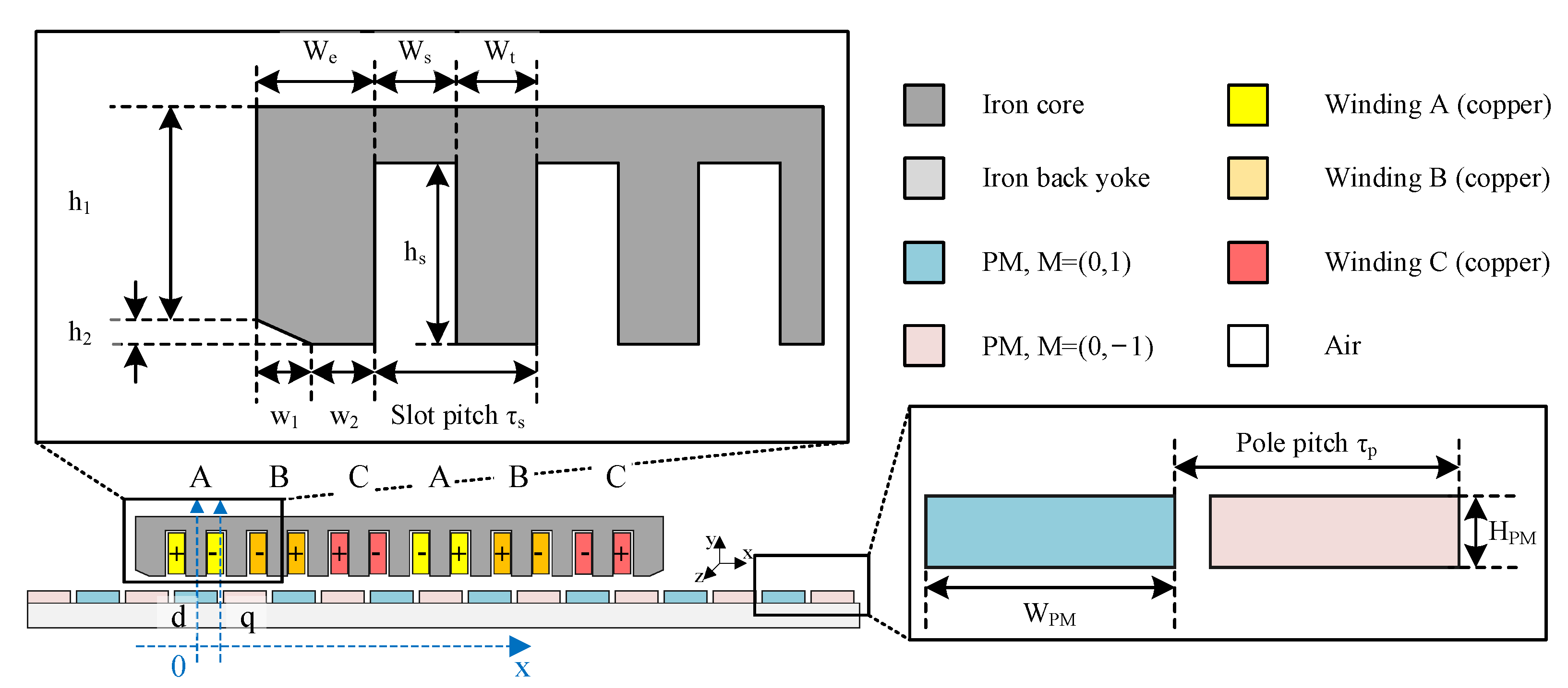
A PMLSM is considered in this study to evaluate the nonlinear material property of the proposed method. The geometry of the PMLSM is shown in Figure 2, the iron core material is Electrical Steel DW310, and the nonlinear B–H curve is shown in Figure 3. The fixed parameters are shown in Table 1.

4.2. Definition of Physics-Based Channels

The channels are defined based on two criteria: (1) Each channel should have a clear and unambiguous physical meaning, and they should consist of the component in each axis or direction if the property is a vector, such as two channels for a 45-degree magnetization vector M = (1, 1) in the 2-D problem and three channels for a z-direction current density J = (0, 0, 100 A/mm2) in the 3-D problem. (2) Different channels should have significant variance in geometric structure or property. These four types of channels are identified in the dataset, as listed below. Figure 1 shows examples of our annotations.
1.
Current density ( J —The current excitation applied to the material on the mesh of the linear motor will be converted to the current density. The number of channels of current density is three in the 3-D problem. In the particular 2-D model, the number of channels of current density can be simplified to one (containing only the vertical direction, such as ( 0 , 0 , J z ) to ( J z ) ) or two (containing any two components, such as ( J x , J y , 0 ) to ( J x , J y ) ) to reduce the storage space occupation.
2.
Magnetization of magnetic materials ( M )—The relative permeability of the magnetic material is close to one, and this material involves channels for the magnetization direction vector. The magnetization will have two channels in the 2-D problem and three in the 3-D problem. If the magnetization has only one direction in the 2-D problem, one channel will be added to reduce the space complexity.
3.
Motion band ( M o t i o n )—The moving part will be marked as 1, and the materials and approximated fields inside the moving band will be extracted after approximation. The number of channels of the motion band is 1.
4.
Permeability of permeable materials ( μ r )—The relative permeability of the permeable material is larger than one. The value of channels of the permeable material is one when the material is isotropic. The anisotropy material will have two channels in 2-D problems and three in 3-D problems.
The dataset contains two parts: the training dataset and the test dataset. The training dataset is used for training the neural network, and the test dataset is used for testing whether the model is well trained for magnetic field approximation.

4.3. Dataset Generation

The dataset is generated from a parametric linear motor model. This model is a conventional PMLSM. The initial configuration is shown in Table 1. The input and output of the neural network are generated by the FEM software. The randomly changing variables of the linear motor model can be found in Table 2.
The boundary condition is the Dirichlet boundary, whose value is 0 weber/m. The distance of the moving speed is set to 1 mm/s. As for the data generation process, all models should be generated from many random parameter combinations.
Six geometric parameters, namely, the width of the edge (We), the width of the slot (Ws), the width of the teeth (Wt), the height of the slot (hs), the pole pitch (τp), and the PM length (WPM), are chosen as the geometry design variables. In addition, the input current also varies from 1 A to 16 A.
The PMLSM training dataset has 5000 samples. The initialization process of a genetic algorithm (GA) is employed to generate initial models since the initialization naturally generates a random combination of given variables, i.e., set the number of maximum populations to 5000 directly.
The PMLSM test dataset has 30 samples. The investigated PMLSM is a flat iron core. Table 3 lists some specifications of the test PMLSM. This PMLSM is a concentrated winding motor with a slot pitch τs = 14 mm, a pole pitch τp = 16 mm, and a force constant Kt = 88.8 N/A. The air gap thickness is about 0.8 mm, and the Neodymium-Iron-Boron (NdFeB) PMs have a residual flux density of approximately 1.23 Tesla. Table 4 demonstrates the content of the test dataset. The test dataset contains all statuses of the test PMLSM, moving from 0 s to 30 s with a speed of 1 mm/s, and each step represents the status every second.

5. Results

This section presents the preliminary results of the PIGAN. The test model is a 2-D PMLSM model, as shown in Table 4. Different FEM results are obtained by moving the iron core to change the position of the mover of the PMLSM model. The geometrical parameters given in Table 1 and Table 3 are considered.
The PIGAN is constructed using TensorFlow 2 [32], trained by a stochastic gradient descent optimizer, Adam [33], with a learning rate of 0.001. Five thousand datapoints from the FEA are preprocessed for the training dataset. The training process takes 200,000 iterations.
In addition, Pix2Pix [27], another cGAN, is implemented for comparison. The loss function of the Pix2Pix uses the L1 loss recommended in the original paper and does not incorporate physical information. All other model parameters and optimization parameters are the same as those in PIGAN.

5.1. Evaluation Metrics

Two types of evaluation metrics are considered in this study, including image synthesis metrics and electromagnetic metrics.

5.1.1. Image Synthesis Metrics

There are no existing metrics for magnetic field synthesis. In order to objectively demonstrate the superiority of the proposed method, all the experiments were quantitatively evaluated using the mean absolute error (MAE), the structural similarity (SSIM) index, and the peak signal-to-noise ratio (PSNR). The MAE, also known as the L1 loss, is a measurement between two paired matrices. It calculates the sum of absolute errors divided by the matrices’ sizes in this study, which are intuitive metrics for similarity measurements. The SSIM index measures the similarity of structural information in two images, where 0 indicates no similarity and 1 indicates total positive similarity. SSIM can be used in physics-based image restoration [34,35,36], and a higher SSIM index means that the synthetic fundus image is closer to the real one. PSNR measures the image distortion and noise level between two images. A higher PSNR value indicates a higher image quality.

5.1.2. Electromagnetic Metric

Magnetic force is one of the most critical performance indicators of linear motors. It can be obtained by flux density.
The force applied to the mover in the x direction F x can be obtained by using the MST method and is given by:
F x = L μ 0 g a p B x ( x a i r , y a i r ) B y ( x a i r , y a i r ) d x
where B x ( x a i r , y a i r ) is the x-component of the flux density in the airgap and B y ( x a i r , y a i r ) is the y-component of the flux density in the airgap of the PMLSM.

5.2. Predicted Results of the Linear Machine

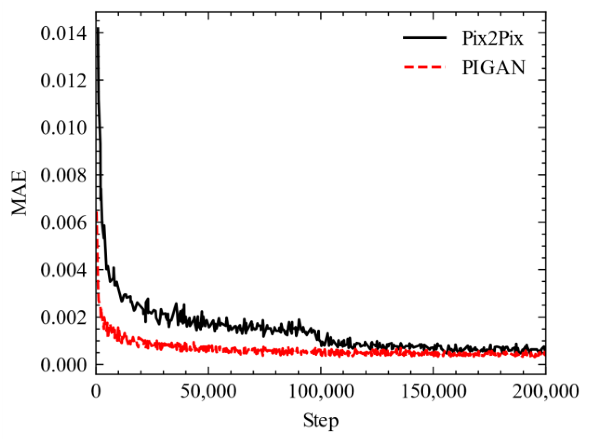
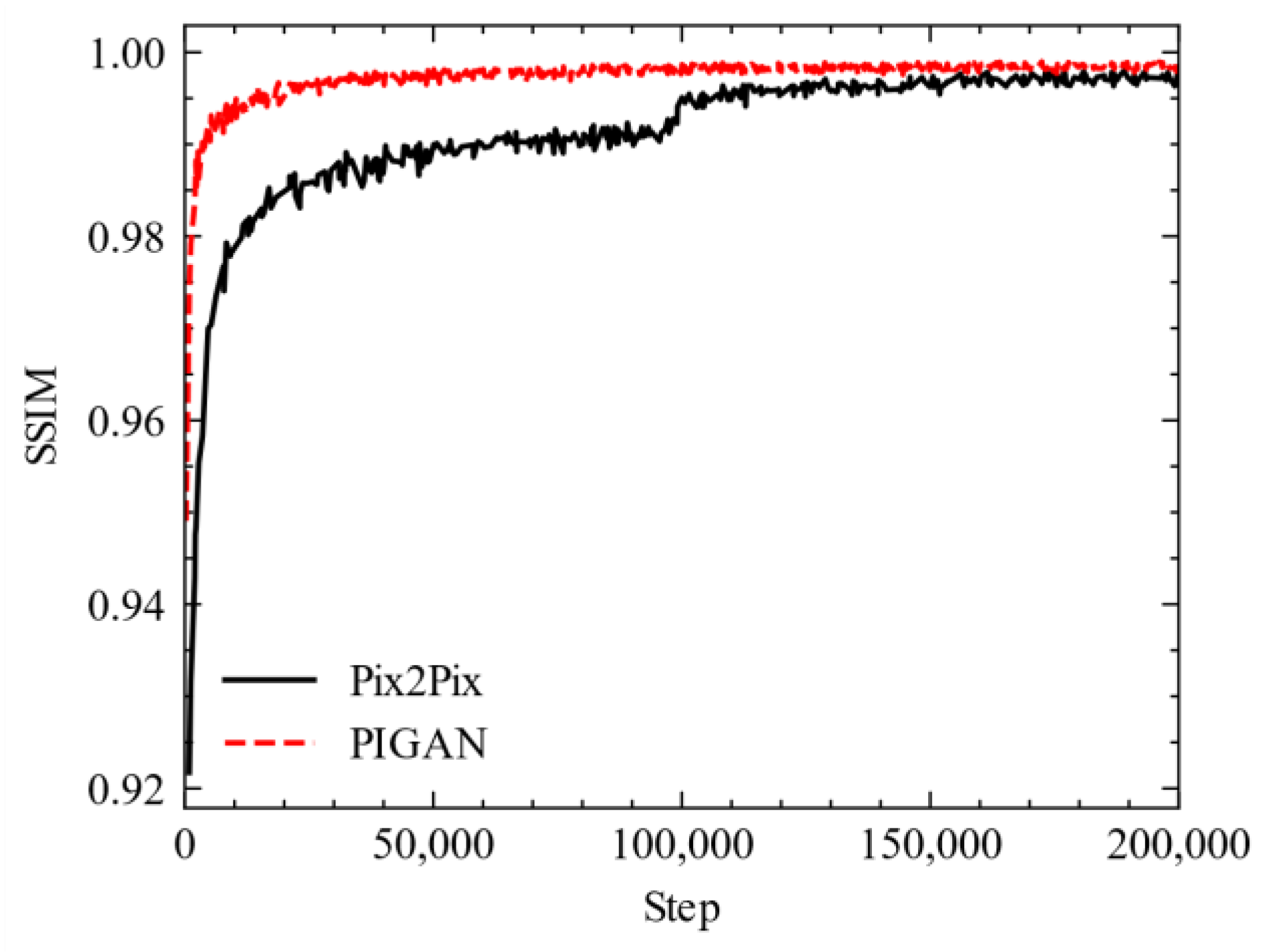
It takes approximately 16 hours of training time for the proposed PIGAN. As for the evaluation process, the total magnetic field approximation time of the 30-step PMLSM model using the proposed PIGAN is 1 s; each step costs 33.3 ms on average. In comparison, the conventional 30-step FE simulation takes 45 s, and each step takes 1.5 s on average. Convergence is achieved in around 150 k to 200 k iterations depending on the network configuration, as shown in Figure 4, Figure 5 and Figure 6.
It can be seen in Figure 4 that the results using Pix2Pix have a higher loss in MAE. The curves of the PSNR and SSIM also show the same conclusion.
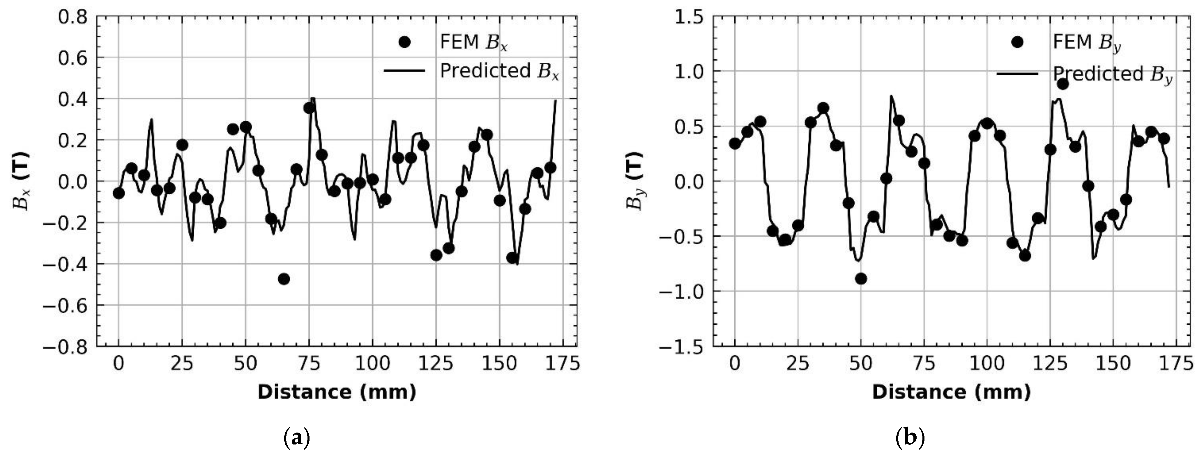
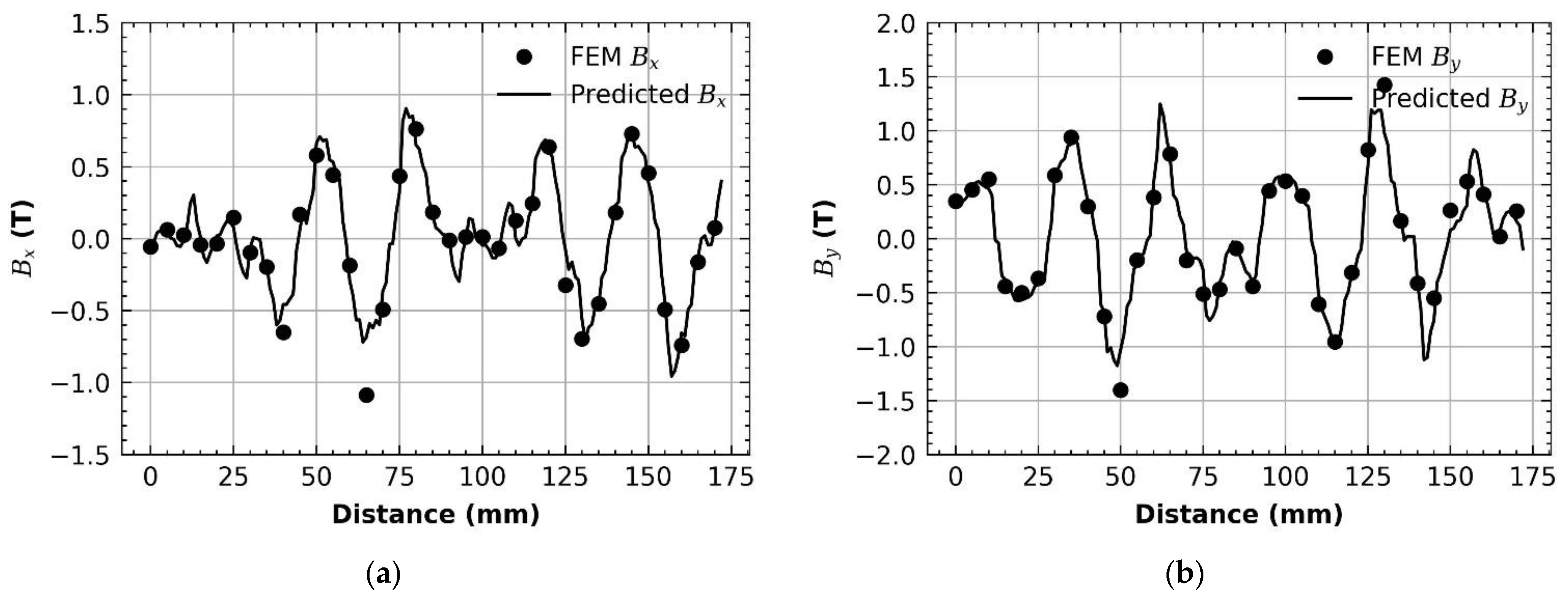
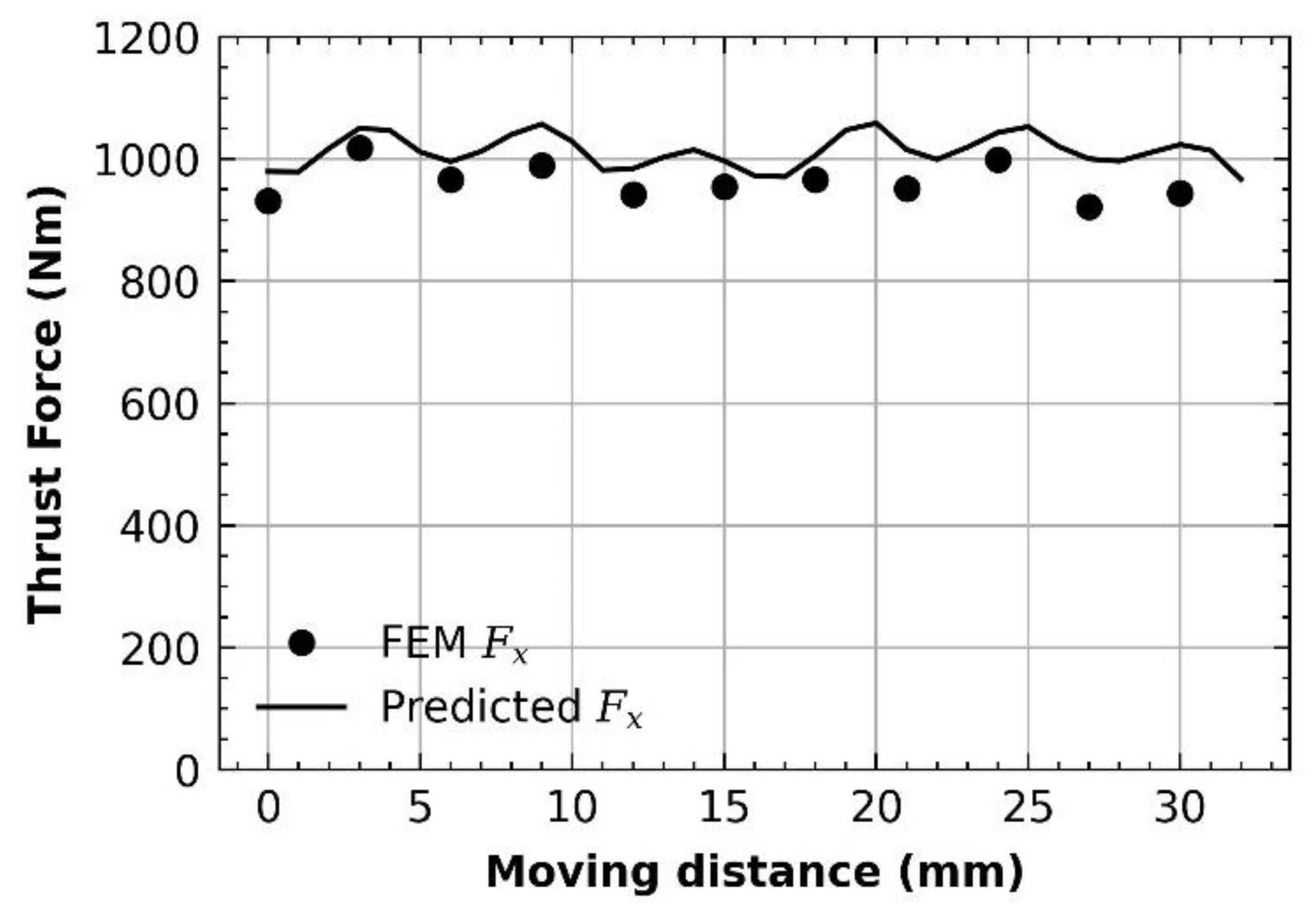
Although the image synthesis metrics of the final optimized models of both PIGAN and Pix2Pix are very close, they differ significantly in the electromagnetic metrics. As shown in Table 5, for the x-axis thrust, with continuous current excitation, the FEM is calculated to be 190 N, the PIGAN is calculated to be 192 N, and the Pix2Pix is calculated to be 150 N, with an error of 21.05%. The same is true for the peak current excitation, with an error of 3.16% for the PIGAN but of 15.79% for the Pix2Pix. The specific PIGAN and FE calculations resulting in the air gap magnetic density distribution and thrust force on the x-axis are shown in Figure 7, Figure 8, Figure 9 and Figure 10. This shows that the loss function based on physical information can benefit the magnetic field approximation.

6. Discussion

In this section, several critical challenges revealed by our proposed dataset are identified, and the possible solutions are explored to overcome them and eventually improve the performance of magnetic field approximation. Note that the aim is not to propose new algorithms in this section. Instead, it is to generalize the existing pipelines from the perspective of dataset characteristics.
A.
3-D problem
For 3-D problems, the input size is at least several hundred times larger than it is for 2-D problems. Suppose the 3-D model with a structured mesh and its magnetic field is approximated using the image synthesis method. In this case, only the newly added axis will cause the number of input variables to be several hundred times, and the number of channels will also increase.
For example, if the axis of input of a 2-D problem is [100, 512, 512, 4], then the equivalent input of the 3-D model is [100, 512, 512, 512, 6] if the length of the z-axis is 512, and two 2-D channels are converted to 3-D channels. Moreover, as for the anisotropic material properties, the 3-D problem will be more complicated
In the future, it is suggested that 3-D problems can be processed as 3-D mesh segmentation or point cloud processing instead of using structured grids such as pictures. The data structure will also be more complicated. It is necessary to arrange the input data structure and memory location reasonably. If it is heterogeneous computing, it is necessary to consider sharing the same memory instead of the existing time-consuming and complex algorithms, such as copying the memory data to the GPGPU memory.
B.
Materials
Nonlinear electromagnetic material is widely used, and researchers have deeply investigated the characteristic for decades. The nonlinear material properties that need to be considered will increase the number of input channels.
In addition, nonlinear materials require proprietary databases and formulas for fitting queries. As for anisotropic materials, the material properties in each direction can be a vectorized property, which is more complicated in data preprocessing. If a multi-physics problem is considered, the model’s input will change because the input dimension, such as the channels, will be added, leading the model being retrained.
C.
Boundary conditions
Boundary conditions (b.c.) are constraints that are necessary to solve a boundary value problem. The significant influence of b.c. is that the input and output of the dataset cannot be cropped simply without the b.c. Our dataset uses the Dirichlet boundary condition, and the value is determined to be zero. Therefore, the initial b.c. channels are neglected in the input.
If a non-zero b.c. is considered, the channels should be added, making the problem even more complex. Some preliminary results [37] show that the image inpainting technique from the computer vision can benefit this issue.
D.
Integration error
When calculating the magnetic force, the integration will be performed, which will enlarge the total error, even if the error of each point is small. For example, the concepts of force and torque using the MST method in the electromagnetic field require producing and integrating the alternating magnetic field near the moving object, and the calculation error rises extremely quickly.
Furthermore, 64-bit floating numbers (FP64) for scientific calculation are pretty common, while machine learning algorithms use 16-bit (FP16) or 32-bit (FP32) floating numbers. The cost-performance ratio will be meager if the dedicated hardware trains the model.

7. Conclusions

In this study, a PIGAN for electromagnetic field approximation is proposed. The proposed method of generating FE model data and defining input channels achieves a better electromagnetic field approximation accuracy. A physics-informed loss function outperforms the naive benchmark models through extensive benchmarking, improving forecasting performance. The mean absolute percentage error of the thrust force between the prediction using the PIGAN and the FE solution is less than 4%. At the same time, the calculation time of the PIGAN is almost forty times faster than that of the FE method. Moreover, several open challenges are highlighted, including 3-D problems for electromagnetic field approximation, material property consideration, and integration error in fundamental performance estimation.
Additionally, the PIGAN, as a neural network, has a standard development process. The standardized development process can significantly reduce the difficulty of software development, and it will be easier to put the PIGAN into industrial applications than FE solvers. With the accumulation of data, the PIGAN can evolve itself to improve its computational accuracy further. The PIGAN is expected to be a steppingstone towards advancing research in related areas.

Author Contributions

Conceptualization, H.W.; Methodology, H.W.; Software, H.W.; Validation, H.W.; Formal Analysis, H.W.; Investigation, H.W.; Resources, Y.Z.; Data curation, Y.Z.; Supervision, S.N. and W.F.; Visualization, H.W.; Writing—original draft, H.W.; Writing—review & editing, S.N.; Project Administration, H.W.; Funding acquisition, S.N. All authors have read and agreed to the published version of the manuscript.

Funding

This research was funded by the Research Grant Council of the Hong Kong Government, grant number PolyU 152109/20E.

Institutional Review Board Statement

Not applicable.

Informed Consent Statement

Not applicable.

Data Availability Statement

Part of the data presented in this study are openly available in LiM2D at DOI: 10.34740/14aggle/dsv/3150834.

Conflicts of Interest

The authors declare no conflict of interest.

References

  1. Li, Y.; Lei, G.; Bramerdorfer, G.; Peng, S.; Sun, X.; Zhu, J. Machine Learning for Design Optimization of Electromagnetic Devices: Recent Developments and Future Directions. Appl. Sci. 2021, 11, 1627. [Google Scholar] [CrossRef]
  2. Wang, H.; Zhang, C.; Yang, Y.; Liang, R.H.W.; Hui, S.Y. A Comparative Study on Overall Efficiency of 2-Dimensional Wireless Power Transfer Systems Using Rotational and Directional Methods. IEEE Trans. Ind. Electron. 2021, 69, 260–269. [Google Scholar] [CrossRef]
  3. Yang, H.; Qian, C.; Wang, W.; Lin, H.; Zhu, Z.Q.; Niu, S.; Liu, W.; Lyu, S. A Novel Asymmetric-Magnetic-Pole Interior PM Machine with Magnet-Axis-Shifting Effect. IEEE Trans. Ind. Appl. 2021, 57, 5927–5938. [Google Scholar] [CrossRef]
  4. Pata, J.; Duarte, J.; Vlimant, J.-R.; Pierini, M.; Spiropulu, M. MLPF: Efficient Machine-Learned Particle-Flow Reconstruction Using Graph Neural Networks. Eur. Phys. J. C 2021, 81, 381. [Google Scholar] [CrossRef]
  5. Jiang, H.; Nie, Z.; Yeo, R.; Farimani, A.B.; Kara, L.B. StressGAN: A Generative Deep Learning Model for Two-Dimensional Stress Distribution Prediction. J. Appl. Mech. Trans. ASME 2021, 88, 051005. [Google Scholar] [CrossRef]
  6. Tresser, S.; Dolev, A.; Bucher, I. Dynamic Balancing of Super-Critical Rotating Structures Using Slow-Speed Data via Parametric Excitation. J. Sound Vib. 2018, 415, 59–77. [Google Scholar] [CrossRef] [Green Version]
  7. Jha, D.; Smedsrud, P.H.; Riegler, M.A.; Johansen, D.; De Lange, T.; Halvorsen, P.; Johansen, H.D. ResUNet++: An Advanced Architecture for Medical Image Segmentation. In Proceedings of the 2019 IEEE International Symposium on Multimedia (ISM), San Diego, CA, USA, 9–11 December 2019; pp. 225–230. [Google Scholar] [CrossRef] [Green Version]
  8. Hanke, S.; Wallscheid, O.; Böcker, J. Data Set Description: Identifying the Physics Behind an Electric Motor—Data-Driven Learning of the Electrical Behavior (Part I). arXiv 2020, arXiv:2003.06268. [Google Scholar]
  9. Kirchgassner, W.; Wallscheid, O.; Bocker, J. Estimating Electric Motor Temperatures with Deep Residual Machine Learning. IEEE Trans. Power Electron. 2021, 36, 7480–7488. [Google Scholar] [CrossRef]
  10. Mcgregor, S.; Dhuri, D.; Berea, A.; Muñoz-Jaramillo, A. FlareNet: A Deep Learning Framework for Solar Phenomena Prediction. In Proceedings of the Workshop on Deep Learning for Physical Sciences (DLPS 2017), NIPS 2017, Long Beach, CA, USA, 8 December 2017; pp. 1–5. [Google Scholar]
  11. Mokhtar, F.; Kansal, R.; Diaz, D.; Duarte, J.; Pata, J.; Pierini, M.; Vlimant, J.-R. Explaining Machine-Learned Particle-Flow Reconstruction. arXiv 2021, arXiv:2111.12840. [Google Scholar]
  12. Ma, Z.; Xu, K.; Song, R.; Wang, C.-F.; Chen, X. Learning-Based Fast Electromagnetic Scattering Solver Through Generative Adversarial Network. IEEE Trans. Antennas Propag. 2020, 69, 2194–2208. [Google Scholar] [CrossRef]
  13. Gong, R.; Tang, Z. Investigation of Convolutional Neural Network U-Net under Small Datasets in Transformer Magneto-Thermal Coupled Analysis. COMPEL—Int. J. Comput. Math. Electr. Electron. Eng. 2020, 39, 959–970. [Google Scholar] [CrossRef]
  14. Wu, H.; Niu, S.; Zhang, Y.; Zhao, X.; Fu, W. Fast Magnetic Field Approximation Method for Simulation of Coaxial Magnetic Gears Using AI. IEEE J. Emerg. Sel. Top. Ind. Electron. 2022, 1–9. [Google Scholar] [CrossRef]
  15. Weinkauf, T.; Theisel, H. Streak Lines as Tangent Curves of a Derived Vector Field. IEEE Trans. Vis. Comput. Graph. 2010, 16, 1225–1234. [Google Scholar] [CrossRef] [PubMed]
  16. Khan, A.; Ghorbanian, V.; Lowther, D. Deep Learning for Magnetic Field Estimation. IEEE Trans. Magn. 2019, 55, 7202304. [Google Scholar] [CrossRef]
  17. Brunton, S.L.; Budišić, M.; Kaiser, E.; Kutz, J.N. Modern Koopman Theory for Dynamical Systems. arXiv 2021, arXiv:2102.12086. [Google Scholar] [CrossRef]
  18. Essien, A.; Giannetti, C. A Deep Learning Model for Smart Manufacturing Using Convolutional LSTM Neural Network Autoencoders. IEEE Trans. Ind. Inform. 2020, 16, 6069–6078. [Google Scholar] [CrossRef] [Green Version]
  19. Lusch, B.; Kutz, J.N.; Brunton, S.L. Deep Learning for Universal Linear Embeddings of Nonlinear Dynamics. Nat. Commun. 2018, 9, 4950. [Google Scholar] [CrossRef] [PubMed] [Green Version]
  20. Mohammadi, M.H.; Ghorbanian, V.; Lowther, D.A. A Data-Driven Approach for Design Knowledge Extraction of Synchronous Reluctance Machines Using Multi-Physical Analysis. In Proceedings of the 2018 23rd International Conference on Electrical Machines, ICEM 2018, Alexandroupoli, Greece, 3–6 September 2018; pp. 479–485. [Google Scholar] [CrossRef]
  21. Kochkov, D.; Smith, J.A.; Alieva, A.; Wang, Q.; Brenner, M.P.; Hoyer, S. Machine Learning Accelerated Computational Fluid Dynamics. Proc Natl. Acad. Sci. USA 2021, 118, e2101784118. [Google Scholar] [CrossRef] [PubMed]
  22. Gong, R.; Tang, Z. Training Sample Selection Strategy Applied to CNN in Magneto-Thermal Coupled Analysis. IEEE Trans. Magn. 2021, 9464, 8–11. [Google Scholar] [CrossRef]
  23. Pollok, S.; Bjork, R.; Jorgensen, P.S. Inverse Design of Magnetic Fields Using Deep Learning. IEEE Trans. Magn. 2021, 57, 2101604. [Google Scholar] [CrossRef]
  24. Doi, S.; Sasaki, H.; Igarashi, H. Multi-Objective Topology Optimization of Rotating Machines Using Deep Learning. IEEE Trans. Magn. 2019, 55, 7202605. [Google Scholar] [CrossRef]
  25. Qi, S.; Wang, Y.; Li, Y.; Wu, X.; Ren, Q.; Ren, Y. Two-Dimensional Electromagnetic Solver Based on Deep Learning Technique. IEEE J. Multiscale Multiphys. Comput. Tech. 2020, 5, 83–88. [Google Scholar] [CrossRef]
  26. Goodfellow, I.; Pouget-Abadie, J.; Mirza, M.; Xu, B.; Warde-Farley, D.; Ozair, S.; Courville, A.; Bengio, Y. Generative Adversarial Networks. Commun. ACM 2020, 63, 139–144. [Google Scholar] [CrossRef]
  27. Isola, P.; Zhu, J.Y.; Zhou, T.; Efros, A.A. Image-to-Image Translation with Conditional Adversarial Networks. In Proceedings of the 30th IEEE Conference on Computer Vision and Pattern Recognition, CVPR 2017, Honolulu, HI, USA, 21–26 July 2017; pp. 5967–5976. [Google Scholar] [CrossRef] [Green Version]
  28. Arora, S.; Ge, R.; Liang, Y.; Ma, T.; Zhang, Y. Generalization and Equilibrium in Generative Adversarial Nets (GANs). In Proceedings of the 34th International Conference on Machine Learning, ICML 2017, Sydney Australia, 6–11 August 2017; Volume 1, pp. 322–349. [Google Scholar]
  29. Remy, G.; Krebs, G.; Tounzi, A.; Barre, P. Finite Element Analysis of a PMLSM (Part 1)—Meshing Techniques and Thrust Computations. In Proceedings of the 6th International Symposium on Linear Drives for Industrial Applications, Lille, France, 16–19 September 2007; pp. 2–5. [Google Scholar]
  30. Remy, G.; Krebs, G.; Tounzi, A.; Barre, P. Finite Element Analysis of a PMLSM (Part 2)—Cogging Force and End-Effect Force Calculations. In Proceedings of the 6th International Symposium on Linear Drives for Industrial Applications, Lille, France, 16–19 September 2007; pp. 2–5. [Google Scholar]
  31. Remy, G.; Krebs, G.; Tounzi, A.; Barre, P.J. Detent Force Calculations of a PMLSM Using the Finite Element Method. IEEJ Trans. Ind. Appl. 2009, 129, 462–469. [Google Scholar] [CrossRef]
  32. Abadi, M.; Barham, P.; Chen, J.; Chen, Z.; Davis, A.; Dean, J.; Devin, M.; Ghemawat, S.; Irving, G.; Isard, M.; et al. TensorFlow: A System for Large-Scale Machine Learning. In Proceedings of the 12th USENIX Symposium on Operating Systems Design and Implementation, OSDI 2016, Savannah, GA, USA, 2–4 November 2016. [Google Scholar]
  33. Kingma, D.P.; Ba, J.L. Adam: A Method for Stochastic Optimization. In Proceedings of the 3rd International Conference on Learning Representations, ICLR 2015, San Diego, CA, USA, 7–9 May 2015; pp. 1–15. [Google Scholar]
  34. Le, M.; Pham, C.T.; Lee, J. Deep Neural Network for Simulation of Magnetic Flux Leakage Testing. Meas. J. Int. Meas. Confed. 2021, 170, 108726. [Google Scholar] [CrossRef]
  35. Pan, J.; Liu, Y.; Dong, J.; Zhang, J.; Ren, J.; Tang, J.; Tai, Y.W.; Yang, M.H. Physics-Based Generative Adversarial Models for Image Restoration and Beyond. arXiv 2018. [Google Scholar] [CrossRef] [Green Version]
  36. Horé, A.; Ziou, D. Image Quality Metrics: PSNR vs. SSIM. In Proceedings of the International Conference on Pattern Recognition, Istanbul, Turkey, 23–26 August 2010; pp. 2366–2369. [Google Scholar] [CrossRef]
  37. Pollok, S.; Olden-Jørgensen, N.; Jørgensen, P.S.; Bjørk, R. Magnetic Field Prediction Using Generative Adversarial Networks. arXiv 2022, arXiv:2203.07897. [Google Scholar]
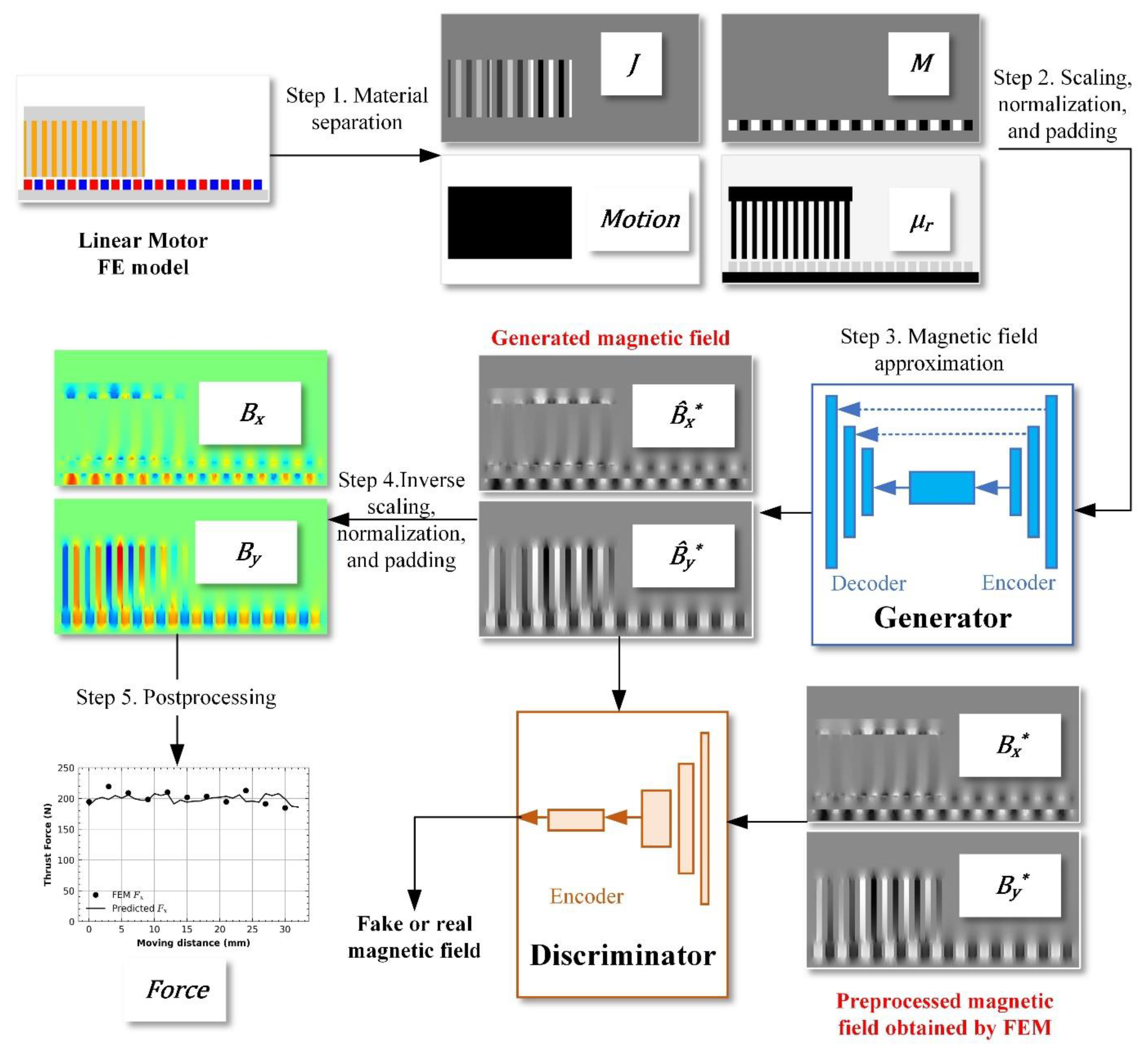
Figure 1. Overview of novel DL approach for magnetic field approximation. A generator is trained to predict the magnetic field values.
Applsci 12 10426 g001
Figure 2. The cutting view and key dimensions of the PMLSM.
Applsci 12 10426 g002
Figure 3. The B-H curve of the steel DW310 in the iron.
Applsci 12 10426 g003
Figure 4. The MAE loss curve of the proposed PIGAN and Pix2Pix.
Applsci 12 10426 g004
Figure 5. The PSNR curve of the PIGAN and Pix2Pix.
Applsci 12 10426 g005
Figure 6. The SSIM curve of the PIGAN and Pix2Pix.
Applsci 12 10426 g006
Figure 7. The prediction and FEM results of the (a) x-axis and (b) y-axis air gap flux density when the PMLSM works with the continuous current (2.23 A).
Applsci 12 10426 g007
Figure 8. The prediction results and FEM results of thrust force when the PMLSM works with the continuous current (2.23 A).
Applsci 12 10426 g008
Figure 9. The prediction and FEM results of the (a) x-axis and (b) y-axis air gap flux density when the PMLSM works with the peak current (15.5 A).
Applsci 12 10426 g009
Figure 10. The prediction and FEM results of the thrust force when the PMLSM works with the peak current (15.5 A).
Applsci 12 10426 g010
Table 1. List of fixed parameters of the PMLSM.
ParameterValueUnit
Winding typeConcentrate Winding-
Number of turns380-
Residual flux density of the PMs1.23T
Number of slots12-
Airgap length0.8mm
Edge Height (h1)17.4mm
Edge Height (h2)2.0mm
Edge Width (w1)4.5mm
Edge Width (w2)5.2mm
Table 2. List of variables of the randomly generated PMLSM model.
VariableMin.Max.Unit
WeEdge of the PMLSM520mm
WsWidth of the slot511mm
hsHeight of the slot815mm
WtWidth of the teeth511mm
τpPole pitch1216mm
WPMPM length1020mm
irmsInput current116A
Table 3. List of geometrical variables of the test PMLSM.
ParameterValueUnit
WeEdge of the PMLSM9.7mm
WsWidth of the slot6.6mm
hsHeight of the slot14.8mm
WtWidth of the teeth6.6mm
τpPole pitch16mm
WPMPM length14mm
Table 4. Examples of our test dataset. The three columns indicate the transient status of a linear motor when it moves at the speed of 1 mm/s from the start point to the endpoint. Each column is the status of the linear motor at the specified time. The first four rows are the preprocessed input, and the last two are the FEM results without scaling.
Time = 0 sTime = 15 sTime = 30 s
ModelApplsci 12 10426 i001Applsci 12 10426 i002Applsci 12 10426 i003
InputMotionApplsci 12 10426 i004Applsci 12 10426 i005Applsci 12 10426 i006Applsci 12 10426 i007
μ r Applsci 12 10426 i008Applsci 12 10426 i009Applsci 12 10426 i010Applsci 12 10426 i011
MApplsci 12 10426 i012Applsci 12 10426 i013Applsci 12 10426 i014Applsci 12 10426 i015
JApplsci 12 10426 i016Applsci 12 10426 i017Applsci 12 10426 i018Applsci 12 10426 i019
OutputBxApplsci 12 10426 i020Applsci 12 10426 i021Applsci 12 10426 i022Applsci 12 10426 i023
ByApplsci 12 10426 i024Applsci 12 10426 i025Applsci 12 10426 i026Applsci 12 10426 i027
Table 5. Comparative study of the magnetic field approximation for the simulation of the test PMLSM using FEM, Pix2Pix, and our model.
FEMPredictionAbsolute Error (%)
Pix2PixPIGANPix2PixPIGAN
Continuous force @ 2.23 A190 N150 N192 N21.05%1.05%
Peak force @ 15.5 A950 N800 N980 N15.79%3.16%
Publisher’s Note: MDPI stays neutral with regard to jurisdictional claims in published maps and institutional affiliations.