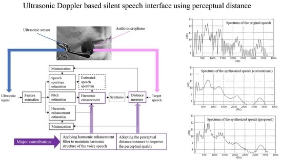
Ultrasonic Doppler Based Silent Speech Interface Using Perceptual Distance

Abstract

Moderate performance in terms of intelligibility and naturalness can be obtained using previously established silent speech interface (SSI) methods. Nevertheless, a common problem associated with SSI has involved deficiencies in estimating the spectrum details, which results in synthesized speech signals that are rough, harsh, and unclear. In this study, harmonic enhancement (HE), was used during postprocessing to alleviate this problem by emphasizing the spectral fine structure of speech signals. To improve the subjective quality of synthesized speech, the difference between synthesized and actual speech was established by calculating the distance in the perceptual domains instead of using the conventional mean square error (MSE). Two deep neural networks (DNNs) were employed to separately estimate the speech spectra and the filter coefficients of HE, connected in a cascading manner. The DNNs were trained to incrementally and iteratively minimize both the MSE and the perceptual distance (PD). A feasibility test showed that the perceptual evaluation of speech quality (PESQ) and the short-time objective intelligibility measure (STOI) were improved by 17.8 and 2.9%, respectively, compared with previous methods. Subjective listening tests revealed that the proposed method yielded perceptually preferred results compared with that of the conventional MSE-based method.

1. Introduction

Silent speech interface (SSI) techniques [1,2] have been proposed to cope with specific situations where voice information should be communicated without the need for actual human vocalization. SSI is also useful for persons with speaking impairment who have suffered permanent vocal damage after an accident or following treatment for laryngeal cancer. These patients, with the help of SSI technology, can produce their own voice by mimicking vocalization. The SSI technique enables voice communication through articulatory movements, rather than by the voice itself, even when voice communication is impossible due to background noise. Techniques associated with SSI also allow persons to speak to one another in a public space, such as a library or conference room without disturbing others. Moreover, it can be useful in situations where others should not be audibly exposed to private information.

A straightforward way to implement SSI is to synthesize voices using a text-to-speech synthesizer (TTS) that accepts text transcription obtained by an automatic speech recognizer (ASR). The features for ASR are derived from the input signals of SSI. In this approach, the intelligibility of the synthesized speech signals is highly affected by the accuracy of the underlying ASR. Moreover, speaker-specific voice characteristics are determined by the underlying TTS.

An alternative way is to directly synthesize voices using the features derived from the input signals of SSI, without using ASR and TTS. SSI is achieved by estimating the mapping rules of the feature parameters derived from the non-acoustic modalities of corresponding voice signals. The non-acoustic modalities adopted for a SSI should be highly correlated with the corresponding audio speech signals and not affected by high levels of ambient audio interference [3]. Various types of modalities satisfying these conditions have been adopted in previously developed SSI methods, such as the Doppler frequency shifts caused by GHz microwaves [4,5,6,7,8], the ultrasound images (UI) of a vocal tract [9,10,11], the visual shape of the mouth [12,13,14,15,16], acoustic Doppler sonic signals [17,18,19,20,21], and signals recorded by a non-audible microphone (NAM) [22,23], or an electromyogram (EMG) [24,25,26,27,28,29,30,31]. Among them, the Doppler-based methods have several advantages over other methods. The problems associated with contact sensing in the EMG- and NAM-based methods can be avoided by non-contact sensing. The Doppler-based techniques are free from image processing-related problems such as inaccuracy in the tracking of regions of the mouth.

The underlying assumption of the Doppler-based SSI methods is that the primary sources of Doppler frequency shifts are vocal vibrations of the body surfaces that cause sounds. A sinusoidal signal with a fixed frequency is incident to a speaker’s mouth and neck regions, and the Doppler shifts of the returned signals are used to synthesize the voice. Our previous study [19] showed that the Doppler-based SSI method using an ultrasonic wave (40 kHz) could be implemented using relatively small and simple hardware by comparison with the use of GHz microwaves and the overall quality of the synthesized speech was superior to other SSI methods and modalities.

The main objective of the present study was to improve the quality of the speech synthesized using the ultrasonic Doppler signal (UDS)-based SSI method. In particular, the perceptual aspects of the reproduced speech were the major concerns of designing the speech estimation rules. In most previous SSI studies [13,21,22,24,25,27,30], the speech signals were represented as Mel-cepstral coefficients (MCCs), which approximated the speech spectrum in the perceptual domain [32]. The objective functions to be minimized in the training stage of those studies was given by the Mel-cepstral distance (MCD). Since the MCC is computed based on human auditory systems, perceptual aspects were considered to some extent in the SSI techniques that were designed to minimize the MCD. In most SSI schemes, however, the differences perceived by the human ear were not directly taken into consideration in construction of the speech estimation rules. Instead, the speech estimation rules were constructed by minimizing the mean squared errors (MSE) between the original and estimated MCCs. This resulted in reproduced speech signals that were less similar to original speech from a perceptual perspective.

Since the reproduced speech from SSI is received by a human ear, it is highly desirable to adopt a human auditory-based distance measure as an objective function. The usefulness of the human auditory-based distance metric has already been verified in various speech processing fields that include speech coding [33], speech enhancement [34], speech recognition [35], speech synthesis [36], and speech quality evaluation [37]. In the proposed SSI method, the speech estimation rules were constructed by minimizing the perceptual differences between the estimated spectra and that of target speech. The perceptual distance was computed in a manner similar to the procedure used to obtain a perceptual evaluation of speech quality (PESQ) [37], which is widely used in speech quality evaluation. And hence, it can be expected that the perceptual qualities of the reproduced speech signals are improved by employing the perceptual distance. In our previous study [19], perceptual aspects were not considered in construction of the speech estimation rules, only the MSE criterion was employed.

Another drawback of the estimation rules adopted in current SSI schemes was that the spectral fine structure was not well estimated, and only an approximated spectrum was obtained. Since the degree of voicing in the vowel- and voiced-consonant regions is closely related to the spectral fine structure, a deficiency in the harmonic spectral structure seriously degrades the intelligibility and naturalness of the reproduced speech, particularly in the voiced regions. To alleviate this problem, both the fundamental frequency ($f_0$) and the voicing state (voiced/unvoiced) have been estimated from a non-acoustic modality to produce a quasi-periodic source signal [22,27,38]. The quality of the voiced regions was partially improved by combining the estimated source signals with a spectral envelope represented by the MCC. However, clear improvements in reproduced speech have not been guaranteed [22,27,30,38]. This was due to severe blurring artifacts of the estimated speech spectrum even though periodic sources were applied [27]. The inaccuracies of f0 estimation and of voiced/unvoiced (V/UV) decisions when using a non-acoustic modality has also been a major reasons for degrading the naturalness of synthesized speech.

In the present study, harmonic enhancement (HE) techniques were adopted to improve the intelligibility and naturalness of synthesized speech. Our previous studies associated with the UDS-based speech enhancement scheme showed that a moderate degree of pitch estimation error was obtained when the pitch periods were predicted using an artificial neural network (ANN) with the features derived from UDS [18]. The perceptual quality of the reproduced speech was improved by HE when a moderate degree of pitch estimation error was maintained [18]. In the subsequent section, we quantitatively analyze the errors of pitch estimation and V/UV decisions for each modality in order to verify the usefulness of non-acoustic pitch estimation. A fixed enhancement factor was adopted in the previous study [18]. In the present study we found, however, that adjusting the enhancement of the harmonic components according to the voicing strength improves the HE. Therefore, the filter coefficients of the HE were determined by UDS in the proposed method. In the training step, two cascade-connected estimators, one for the speech spectrum and one for the HE filter coefficients, were alternatively established to reduce the unique objective function. Such a process can compensate for the estimation errors from one step to another, which thereby reduces the overall error.

The remainder of the paper is organized as follows. First, Section 2 explains the procedure of the baseline SSI system and the limitations. Possible solutions for the problems are explained and the accuracies of the pitch estimation and V/UV decisions are also presented in Section 2. The proposed method is described in Section 3, which includes construction of the speech estimation rules and the HE filter. Experimental results are shown in Section 4. Finally, conclusions are drawn in Section 5.

2. Baseline UDS-Based SSI

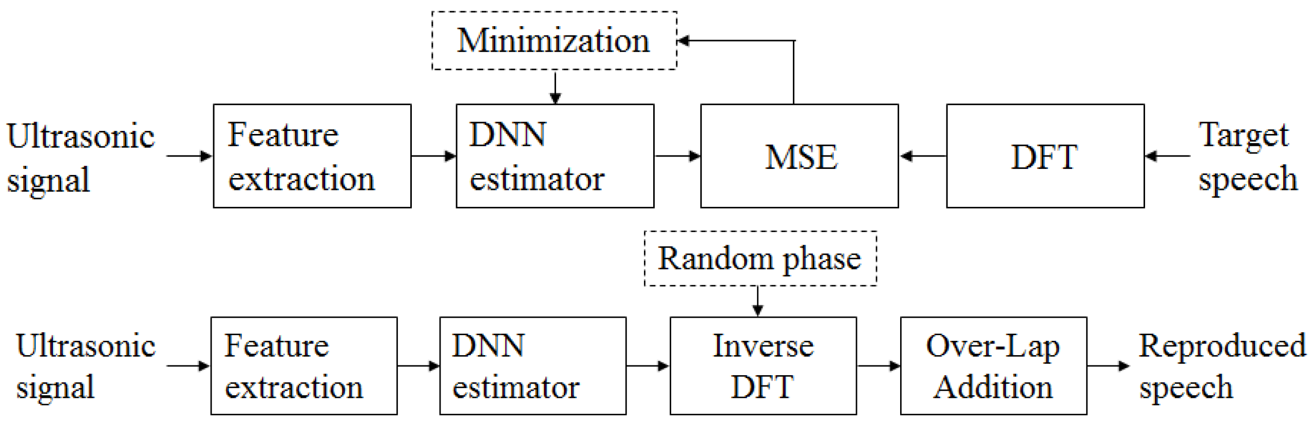
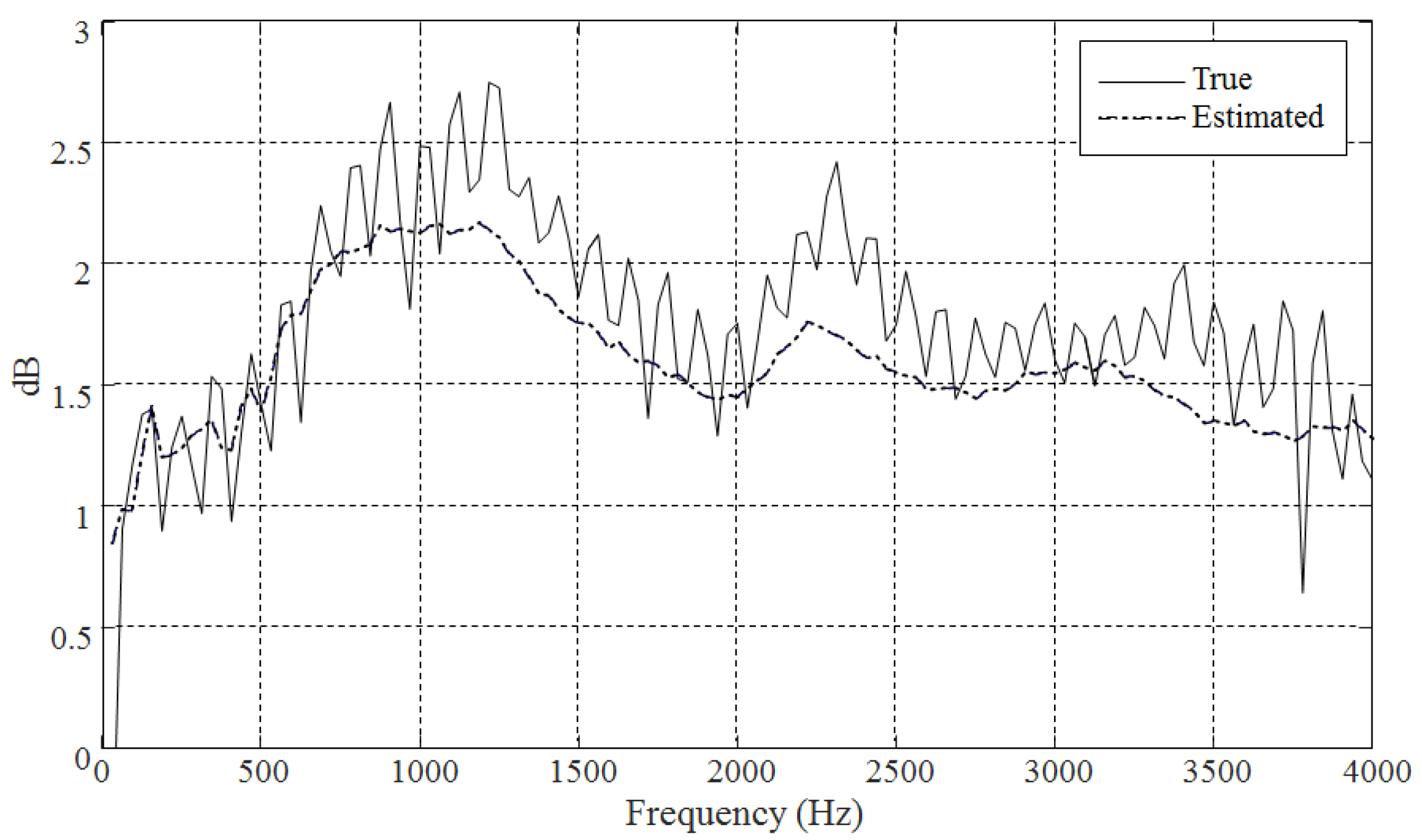
2.1. Estimating the Speech Spectrum

When the ultrasonic tone with a frequency $f_c$ is reflected on an articulating face, Doppler frequency shifts that are potentially caused by the movements of articulatory organs appear in the reflected signals. Assuming that M objects are engaged with the Doppler frequency shift, the instantaneous velocity of the m-th object at time t is then given by $v_m\left(t\right)$, and the reflected signal is given by

$$\begin{array}{ccc}\hfill R\left(t\right)& =& \sum _{m=1}^M{A}_T{k}_{m}cos({\varphi }_m+{\Psi }_T),\hfill \\ \hfill {\varphi }_m& =& 2\pi f_c\left[t+\frac{2}{v_s}{\int }_0^t{v}_m\left(\tau \right)d\tau \right]+{\Psi }_m\hfill \end{array}$$

(1)

where $k_m$ and ${\Psi }_m$ are the attenuation coefficient and phase shift of the m-th object at frequency $f_c$, respectively. $A_T$ and ${\Psi }_T$ are the amplitude and phase of the transmitted sinusoid, and $v_s$ is the speed of sound. The principle of the ultrasound-based speech estimator is that the variables ($k_m$ and ${\Psi }_m$) associated with the Doppler frequency shifts are highly correlated with the underlying speech signals. A block diagram of a baseline UDS-based SSI with deep neural networks (DNN) is shown in Figure 1 where the training procedure and the synthesis procedure are presented at the top and the bottom, respectively. The first step of UDS-based speech estimation is to extract the features from the received ultrasonic signal (US). Our previous study [18] showed that compared with other parameters, the mel-frequency filter bank energies of a demodulated US signal yielded a superior performance in prediction of speech parameters. The bandwidth of the demodulated ultrasonic signal was 2 kHz, and was determined according to the maximum frequency of articulatory movements. The resultant number of mel-bands was 16.

A supervised learning framework was adopted to estimate the relationship between the input UDS and the output speech. In the training stage, a regression DNN model was trained from a training corpus, that consisted of pairs of audio and ultrasound signals. Speech represented by the log magnitude spectra was the target output of the DNN. In the estimation stage, the feature parameters derived from the ultrasound signals were inputted to the trained DNN. The short-time estimated speech signal was obtained by inverse Fourier transform using the output of the DNN, which was the estimated speech spectrum, and the random phase spectrum. Finally, continuous waveforms were obtained by concatenating the short-time estimated speech signals. using the OverLap and Addition (OLA) method.

A back-propagation algorithm is typically used to train a DNN. The objective function is given by a mean square error between the estimated log magnitude spectrum and that of original speech, as follows:

$$E=\frac{1}{N}\sum _{n=1}^N\sum _{p=1}^P{\left\{{\mathcal{F}}_p(\mathbf{W},{\mathbf{x}}_n)-Y_{p,n}\right\}}^2$$

(2)

where ${\mathcal{F}}_p(\mathbf{W},\mathbf{x})$ is the p-th output of the DNN with the weights $\mathbf{W}$ where the input UDS features $\mathbf{x}$ are given. $Y_{p,n}$ denotes the p-th frequency bin of the log-spectral feature at frame index n. A stochastic gradient descent algorithm was performed in mini-batches with multiple epochs to improve the learning convergence. An updated estimate of the weights $\mathbf{W}$ with a learning rate $\lambda$ was computed iteratively as follows:

$${\mathbf{W}}_{n+1}={\mathbf{W}}_n-\lambda {▽}_{\mathbf{W}}E$$

(3)

The DNN captures the acoustic context information along the time axis by adopting multiple frames of ultrasonic signals over time as DNN input [39]. In the present study, the number of neighboring frames was heuristically determined to be 5 by maximizing the performance in terms of speech estimation.

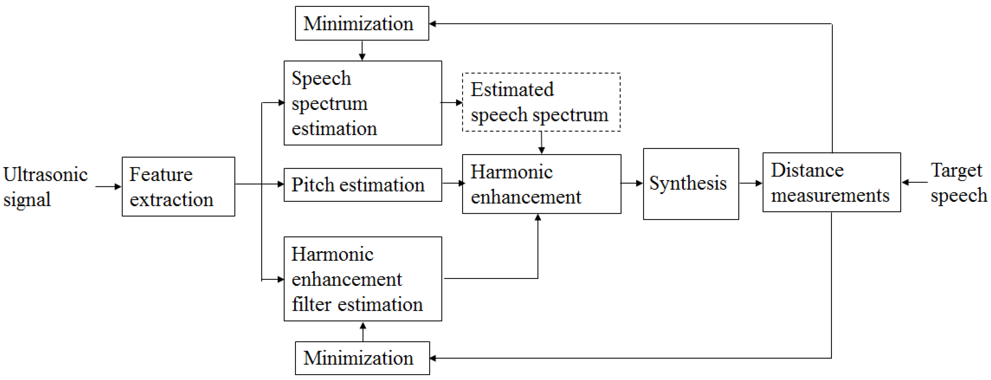
2.2. Harmonic Enhancement

The speech production principle dictates that a speech signal is generated by exciting a vocal tract transfer function via source signals that correspond to the spectral envelope and to the fine structure, respectively, in the frequency domain. The spectral envelope is typically represented using the MCCs, that are predicted from the non-acoustic signals in most SSI systems. The source signals originate either from white noise (for unvoiced regions) or from impulse train signals (for voiced regions). Artificially generated signals, such as white noise [12,25,30], an impulse train with a constant pitch period [12], and an impulse train with randomly perturbed pitch periods [12] were adopted as source signals in previous SSI methods. Such artificially generated source signals do not originate from natural speech, which leads to reproduced speech signals that sound unnatural.

In the present study, we adopted a method for predicting the entire speech spectra (not only the spectral envelope), which avoided the problems associated with the use of an artificial source signal. The experimental results, however, showed that only spectral envelopes were estimated even when the target output was set as the entire speech spectra. An example of the predicted speech spectrum is shown in Figure 2. This result was commonly observed in most voiced regions. Using such an estimated spectra to synthesize the speech signals resulted in unclear, rough, and unnatural qualities, as experienced in previous studies that used the artificial source signals.

To improve the quality of the reproduced speech signals without the use of artificially generated source signals, harmonic enhancement (HE) [40] was employed in the present study. The main objective of employing HE is to increases the natural quality and clarity of synthesized speech. This can be achieved by emphasizing the periodicity of speech that is typically observed in the voiced regions. The harmonic-enhanced signal $\tilde{y}\left(t\right)$ is given by

$$\tilde{y}\left(t\right)=y\left(t\right)+\sum _{k=-K}^K{\gamma }_k·y(t-P\left(t\right)-k)$$

(4)

where ${\left\{{\gamma }_k\right\}}_{k=-K}^K$ denotes the coefficients of HE and $2K+1$ is the number of taps of the HE filter. By changing ${\gamma }_k$, it is possible to adjust the voicing strength. $P\left(t\right)$ is the pitch period at time t. The HE technique adjusts the periodicity of the speech signals that have already been synthesized without using artificial source signals. The usefulness of HE was verified in the previous US-based SSI method [18].

Although it was apparent that the HE method allows for pitch error [18], a reliable estimation of the pitch period is essential for HE. Evaluation of the performance of pitch estimation and voiced/unvoiced decisions for the various modalities are described in the subsequent section. The accuracy of the ultrasonic signal was compared with that of other modalities so that the usefulness of HE adopted in the US-based SSI system was verified.

2.3. Performance of Pitch Estimation and V/UV Decisions

In most of the current pitch estimation methods, the pitch period is estimated from the audible speech that is not available in the SSI systems [32,41]. The pitch estimation methods using non-audible signals were investigated in the previous SSI studies in which EMG was used [22,27,38]. V/UV decisions using EMG were also proposed in at least one other study [38]. In these studies, the quality of the reproduced speech signals using impulse trains with the estimated pitch periods was investigated. However, neither the quantitative analysis of the pitch estimation accuracy nor the V/UV decision errors were sufficiently discussed in the previous studies.

In the present study, experiments were performed to verify the possibility of pitch estimation and V/UV decisions using lip images, EMG, and ultrasonic signal. A pitch estimation method using non-acoustic signals was proposed in our pervious study [18], where a DNN was trained using a set of the features derived from the non-acoustic signals and the ground truth pitch periods that are detected by audible speech. This method was similar to the previous DNN-based pitch estimation method [41] in which a DNN provided the likelihood of each of the candidate pitch periods, and a sequence of the optimal pitch periods was obtained via a Viterbi-trellis search. In the original work [41], spectral feature vectors derived from noisy speech were inputted to a DNN. In the present study, however, feature vectors derived from the non-acoustic signals were inputted to a DNN. All necessary parameters for pitch estimation such as the number of candidate pitch periods, the weights for the posterior probability, and the transition probability were independently determined for each modality so that the overall accuracy was maximized. A DNN was also employed to implement V/UV decisions given by two output nodes, and each output node corresponded to either the voiced frame or the unvoiced frame.

The performance of pitch estimation and V/UV decision-making was evaluated for each modality by using a validation dataset that was constructed from the three subjects (two males and one female). Each subject pronounced 60 isolated Korean words 10 times. This resulted in a total of 25,232 stimuli that split into 17,904 stimuli for training and 7328 stimuli for the actual test. Although the samples for each modality were not recorded simultaneously (because of changes in the shapes of the mouth region by attaching the EMG electrodes), the differences in speech signals among the modalities were minimized by using the common utterance set and asking the subjects to pronounce each word in a consistent manner. The performance of pitch estimation was evaluated using the two standard metrics: the gross pitch error (GPE) rate and the fine pitch error (FPE) [42]. The GPE frames are defined as voiced frames where the error between the estimated pitch period and the ground truth is greater than 0.625 ms. The GPE rate is then given by

$${\mathrm{GPE}}_{\mathrm{rate}}=\frac{N_{\mathrm{GPE}}}{N_v}$$

(5)

where $N_{\mathrm{GPE}}$ and $N_v$ denote the number of GPE frames and voiced frames, respectively. The FPE is represented by using the mean (${\mu }_{\mathrm{FPE}}$) and the standard deviation (${\sigma }_{\mathrm{FPE}}$) that reflect the bias in the $f_0$ estimation and the accuracy, respectively.

$$\begin{array}{ccc}\hfill {\mu }_{\mathrm{FPE}}& =& \frac{1}{N_v}\sum _{i=1}^{N_v}{ϵ}_i\hfill \end{array}$$

(6)

$$\begin{array}{ccc}\hfill {\sigma }_{\mathrm{FPE}}& =& \sqrt{\frac{1}{N_v}\sum _{i=1}^{N_v}{({ϵ}_i-{\mu }_{\mathrm{FPE}})}^2}\hfill \end{array}$$

(7)

$$\begin{array}{ccc}\hfill {ϵ}_i& =& |\widehat{f_0^i}-f_0^i|,\hfill \end{array}$$

(8)

where $\widehat{f_0^i}$ and $f_0^i$ denote the estimate and the ground truth of $f_0$, respectively, at the i-th frame in the voiced frames.

The experimental results are summarized in

Table 1. Pitch estimation accuracy for each modality.

Modality	FPE $\mathit{\mu }$ [Hz]	FPR $\mathit{\sigma }$ [Hz]	GPE Rate (%)
Vision	48.82	39.95	73.6
EMG	60.19	34.13	88.5
e UDS	27.39	39.33	45.6

. Although the performance of UDS-based pitch estimation is not as high as the speech-based pitch estimation (typically, ${\mathrm{GPE}}_{\mathrm{rate}}<20\%$ for clean speech signal [42]), the superiority of the UDS signal in terms of pitch estimation is clearly found for all metrics. Such results suggest that UDS provides more useful information for pitch estimation. The relationship between the accuracy of the pitch estimation and the quality improvements gained by HE was not analyzed quantitatively. Nevertheless, a high degree of accuracy for the UDS-based pitch estimation would be helpful in improving the quality of the reproduced speech signals when the HE technique is adopted.

Similar trends were observed in the V/UV decisions, as shown in

Table 2. Voiced/unvoiced detection accuracy for each modality.

Modality	Voiced Frames (%)			Unvoiced Frames (%)
	Precision	Recall	Accuracy	Precision	Recall	Accuracy
Vision	84.7	95.4	90.1	74.6	43.7	59.2
EMG	78.8	99.9	89.4	17.0	0.01	8.5
UDS	87.7	88.5	88.1	76.4	74.9	75.7

. For the voiced frames, there was no remarkable difference in overall accuracy among the three modalities. However, the results clearly showed that more reliable detection of the unvoiced frames can be achieved by the UDS signal. The V/UV information is an important parameter that determines whether to apply the harmonic enhancement technique to a given speech frame. In other words, an incorrect decision in the unvoiced regions potentially leads to an unnecessary harmonic emphasis on many unvoiced regions, which degrades the overall quality of the reproduced speech signals. The results indicate the artifacts caused by inadequate harmonic emphasis can be reduced to some extent, by using the UDS-based V/UV decisions.

3. Proposed UDS-Based SSI

3.1. Joint Minimization Using Iterative Learning

A block diagram of the proposed SSI method is shown in Figure 3. The major difference from the baseline SSI shown in Figure 1 is that the objective function to be minimized is given by not only the MSE but also the perceptual distance. In this study, the magnitude spectrum, the HE filter coefficients, and the pitch period were predicted from the features derived from the UDS. To estimate the pitch period, we adopted the approach explained in the previous section. Let ${\mathcal{F}}_Y$ and ${\mathcal{F}}_{\Gamma }$ denote the prediction rules for the magnitude spectrum $\mathbf{Y}$ and the HE filter coefficients $\Gamma$, respectively, and then the optimal prediction rules for the MSE-based methods, ${\mathcal{F}}_Y^{\ast }$, ${\mathcal{F}}_{\Gamma }^{\ast }$ are given by

$$\begin{array}{ccc}\hfill {\mathcal{F}}_Y^{\ast }& =& arg\underset{{\mathcal{F}}_Y}{min}{D}_{MSE}(\mathbf{Y},\widehat{\mathbf{Y}}),\hfill \\ \hfill {\mathcal{F}}_{\Gamma }^{\ast }& =& arg\underset{{\mathcal{F}}_{\Gamma }}{min}{D}_{MSE}(\Gamma ,\widehat{\Gamma })\hfill \end{array}$$

(9)

where $\widehat{\mathbf{Y}}={\mathcal{F}}_Y\left(\mathbf{X}\right)$ and $\widehat{\Gamma }={\mathcal{F}}_{\Gamma }\left(\mathbf{X}\right)$. $\mathbf{X}={\left\{{\mathbf{x}}_n\right\}}_{n=1}^N$ is the set of the UDS features where N is the total number of the features for constructing the prediction rules. $\mathbf{Y}$ and $\Gamma$ are the sets of the magnitude spectra and the HE filter coefficients, respectively, which are obtained from the speech signals. $D_{MSE}(X,Y)$ denotes the MSE between X and Y. Hence, Equation (9) indicates that the prediction rules for two parameters are independently obtained by minimizing each MSE. In the proposed method, construction of the two prediction rules was achieved by jointly minimizing a unique distance measurement as shown in Figure 3.

$${\mathcal{F}}_Y^{\ast },{\mathcal{F}}_Y^{\ast }=arg\underset{{\mathcal{F}}_Y,{\mathcal{F}}_{\Gamma }}{min}{D}_{PD}(\mathbf{Y},\widehat{\mathbf{Y}},\Gamma ,\widehat{\Gamma })$$

(10)

where $D_{PD}$ is the perceptual distance measure that was explained in the subsequent section. Simultaneous minimization of ${\mathcal{F}}_Y^{\ast }$ and ${\mathcal{F}}_{\Gamma }^{\ast }$ cannot be achieved with a closed-form solution, and an iterative method was employed in this study, wherein each prediction rule was iteratively updated to minimize the objective function. Beginning with the initial rules ${\mathcal{F}}_Y^{\left(0\right)}$ and ${\mathcal{F}}_{\Gamma }^{\left(0\right)}$, the conversion rules for each parameter at the n-th iteration are given by

$$\begin{array}{ccc}\hfill {\mathcal{F}}_Y^{\left(i\right)}& =& arg\underset{{\mathcal{F}}_Y}{min}{D}_{PD}\left\{\mathbf{Y},{\mathcal{F}}_Y\left(\mathbf{X}\right),\Gamma ,{\mathcal{F}}_{\Gamma }^{(i-1)}\left(\mathbf{X}\right)\right\}\hfill \\ \hfill {\mathcal{F}}_{\Gamma }^{\left(i\right)}& =& arg\underset{{\mathcal{F}}_{\Gamma }}{min}{D}_{PD}\left\{\mathbf{Y},{\mathcal{F}}_Y^{\left(i\right)}\left(\mathbf{X}\right),\Gamma ,{\mathcal{F}}_{\Gamma }\left(\mathbf{X}\right)\right\}\hfill \end{array}$$

(11)

The process is repeated until some convergence threshold is reached. One of the advantages gained by a method that uses such an iterative construction is that it can compensate for the estimation errors at one step or another, thereby further reducing the overall estimation error.

3.2. Perceptual Distance

In the previous SSI methods, the speech parameters were obtained by minimizing the mean squared error (MSE). Although the resultant speech parameters approximated those of the original speech signals, there was no guarantee that the reproduced speech signals would be perceived as the original speech. In the present study, the conventional MSE-based objective function was modified by incorporating both a symmetrical disturbance $D^{\left(s\right)}$ and an asymmetrical disturbance, $D^{\left(a\right)}$ [34]

$$D_{PD}=\frac{1}{N}\sum _n\left(w_M{D}_{MSE,n}+w_s{D}_n^{\left(s\right)}+w_a{D}_n^{\left(a\right)}\right)$$

(12)

where $D_{MSE}\left(n\right)$ is the MSE of the n-th spectrum

$$D_{MSE,n}=\frac{1}{M}\sum _{m=0}^{M-1}\frac{1}{{\sigma }_m^2}{\left(log\frac{|P_{m,n}{|}^2}{|{\widehat{P}}_{m,n}{|}^2}\right)}^2$$

(13)

where $|P_{m,n}{|}^2$ and $|{\widehat{P}}_{m,n}{|}^2$ are, respectively, the original and predicted power spectra where the indexes, m and n denote frequency and frame, respectively. ${\sigma }_m$ is the standard deviation of $|P_m{|}^2$ and M is the number of frequency bins. In (12), $w_M$, $w_s$, and $w_a$ are weighting factors for the MSE, and the symmetrical and asymmetrical disturbances, respectively. The symmetrical disturbance reflects the absolute difference between the converted and target loudness spectra when auditory masking effects are account for. When the symmetrical disturbance is applied to a SSI, it can be regarded as a distance function between the estimated and target speech represented in a domain that reflects the human auditory system. There are two types of difference patterns in a SSI, one where the target value is greater than the estimated value and vice-versa. Such difference patterns cannot be reflected in distance metrics such as the MSE or the the symmetrical disturbance. Whereas the signs of the loudness differences are considered in the asymmetrical disturbance, the negative differences (under-estimation case) and positive differences (over-estimation case) are perceived differently due to the masking effects. By using the asymmetrical disturbance, the differences between the estimated and target speech signals can be described in more detail, which can lead to an improvement in the SSI performance.

The calculation of symmetrical and asymmetrical disturbances reflects the human auditory system and is composed of several steps, as follows [34]:

(1)

Perceptual domain transformation: The target and converted loudness spectra ${\mathbf{s}}_n={[S_{0,n},\cdots ,S_{Q-1,n}]}^T$ and ${\widehat{\mathbf{s}}}_n={[{\widehat{S}}_{0,n},\cdots ,{\widehat{S}}_{Q-1,n}]}^T$, which are perceptually closer to human listening are obtained as follows,

$${\mathbf{s}}_n=T_s[{\mathbf{H}}^{\left(bt\right)}·{\mathbf{p}}_n],{\widehat{\mathbf{s}}}_n=T_s[{\mathbf{H}}^{\left(bt\right)}·{\widehat{\mathbf{p}}}_n]$$

(14)

where Q is the number of Bark bands, ${\mathbf{H}}^{\left(bt\right)}$ is a Bark transformation matrix that converts the power spectra ${\mathbf{p}}_n=[P_{0,n},\cdots ,P_{M-1,n}]$, ${\widehat{\mathbf{p}}}_n=[{\widehat{P}}_{0,n},\cdots ,{\widehat{P}}_{M-1,n}]$ into the Bark spectra ${\mathbf{b}}_n=[B_{0,n},\cdots ,B_{Q-1,n}]$ and ${\widehat{\mathbf{b}}}_n=[{\widehat{B}}_{0,n},\cdots ,{\widehat{B}}_{Q-1,n}]$, respectively. $T_s[·]$ is a mapping function that converts each band of the Bark spectrum to a sone loudness scale. A detailed description of this function is found in [34].

(2)

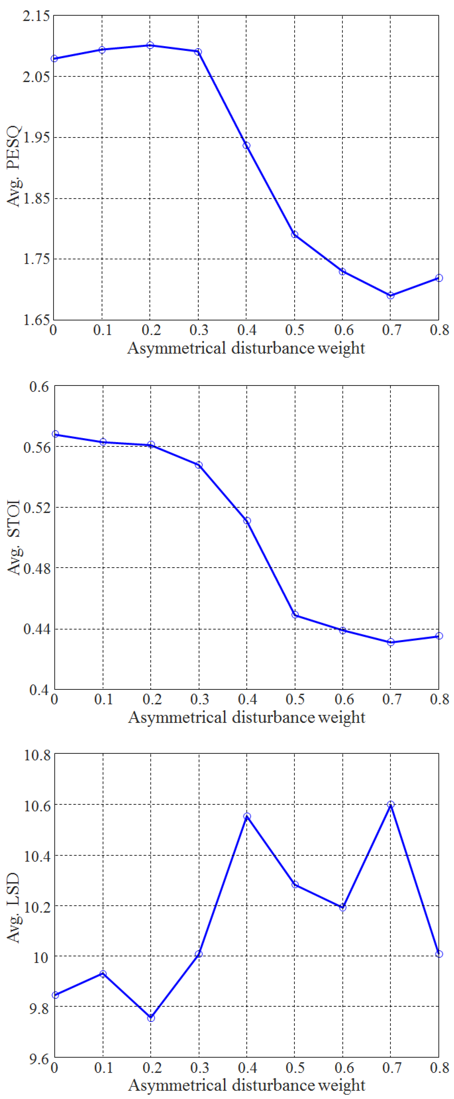
Disturbances computation: A center-clipping operator over the absolute difference between the loudness spectra was applied to compute the symmetrical disturbance vector as follows,

$${\mathbf{d}}_n^{\left(s\right)}=max\left(\right|{\widehat{\mathbf{s}}}_n-{\mathbf{s}}_n|-{\mathbf{m}}_n,\mathbf{0})$$

(15)

where ${\mathbf{m}}_n=0.25·min({\widehat{\mathbf{s}}}_n,{\mathbf{s}}_n)$ is a clipping factor and $|·|$, $min(·)$, and $max(·)$ are applied element-wise. The designation $\mathbf{0}$ is a zero-filled vector of length Q. The asymmetrical disturbance vector is obtained as ${\mathbf{d}}_n^{\left(a\right)}={\mathbf{d}}_n^{\left(s\right)}\odot {\mathbf{r}}_n$, where ⊙ denotes an element-wise multiplication and ${\mathbf{r}}_n$ is a vector of asymmetry ratios the components of which are computed from the Bark spectra.

$$R_{n,q}={\left(\frac{{\widehat{B}}_{q,n}+ϵ}{B_{q,n}+ϵ}\right)}^{\lambda }$$

(16)

For the speech enhancement task, the constants $ϵ$ and $\lambda$ were set to 50 and 1.2, respectively [34]. In the present study, experiments were performed to optimally determine the two constants, $ϵ$ and $\lambda$, minimizing minimize the overall PD. The experimental results show that the same values adopted in [34] also yielded the minimum $D_{\mathrm{PD}}$. The symmetrical and asymmetrical disturbance terms in (12) are given by the weighted sum of each disturbance vector,

$$\begin{array}{ccc}\hfill D_n^{\left(s\right)}& =& \left|\right|{\mathbf{w}}_b{\left|\right|}_1^{\frac{1}{2}}·\left|\right|{\mathbf{w}}_b\odot {\mathbf{d}}_n^{\left(s\right)}{\left|\right|}_2\hfill \\ \hfill D_n^{\left(a\right)}& =& \left|\right|{\mathbf{w}}_b\odot {\mathbf{d}}_n^{\left(a\right)}{\left|\right|}_1={\mathbf{w}}_b^T·{\mathbf{d}}_n^{\left(a\right)}\hfill \end{array}$$

(17)

where the components of the weight vector ${\mathbf{w}}_b$ is proportional to the width of the Bard bands, as explained in [37].

3.3. Estimation of the Prediction Rules

A DNN was used to build the prediction rules ${\mathcal{F}}_Y$ and ${\mathcal{F}}_{\Gamma }$, which map the features derived from the UDS to the magnitude spectrum of the speech signal and the filter coefficients of HE, respectively. The optimum prediction rules were obtained by minimizing the PD between the original power spectra ${\mathbf{p}}_n$ and the predicted power spectra ${\widehat{\mathbf{p}}}_n$. The predicted power spectrum is given by

$${\widehat{\mathbf{p}}}_n={\widehat{\mathbf{y}}}_n\odot {\mathbf{H}}^{\left(he\right)}(P_n,{\Gamma }_n)$$

(18)

where ${\widehat{\mathbf{y}}}_n=[{\widehat{Y}}_{0,n},\cdots ,{\widehat{Y}}_{M-1,n}]$ denotes the magnitude spectra of the predicted speech. ${\mathbf{H}}^{\left(he\right)}(P,\Gamma )$ is the magnitude response of the HE filter for a given pitch period P and the HE filter coefficients $\Gamma ={\left\{{\gamma }_k\right\}}_{k=-K}^K$, which are given by

$$H^{\left(he\right)}(\nu ;P,\Gamma )=|1+\sum _{k=-K}^K{\gamma }_{k}exp\left\{j\pi \nu \right(P+k\left)\right\}|$$

(19)

where $\nu$ is the normalized frequency index, that ranges from 0 to 0.5. With ${\mathbf{W}}_Y$ and ${\mathbf{W}}_{\Gamma }$ as the DNN weights of the predictors ${\mathcal{F}}_Y$ and ${\mathcal{F}}_{\Gamma }$, respectively, the updated estimate of the DNN weights for each predictor can be computed iteratively, and are given by

$$\begin{array}{ccc}\hfill {\mathbf{W}}_Y^{(n+1)}& =& {\mathbf{W}}_Y^{\left(n\right)}-{\lambda }_Y{\nabla }_{{\mathbf{W}}_Y}{D}_{PD}\hfill \\ \hfill {\mathbf{W}}_{\Gamma }^{(n+1)}& =& {\mathbf{W}}_{\Gamma }^{\left(n\right)}-{\lambda }_{\Gamma }{\nabla }_{{\mathbf{W}}_{\Gamma }}{D}_{PD}\hfill \end{array}$$

(20)

where ${\lambda }_Y$ and ${\lambda }_{\Gamma }$ are the learning rates for the weights ${\mathbf{W}}_Y$ and ${\mathbf{W}}_{\Gamma }$, respectively.

3.4. Speech Synthesis

As the final step of the UDS-based SSI system, an audible speech signal is synthesized using the speech parameters predicted from the UDS features. An approach based on a linear prediction (LP) model was adopted in the previous studies, where a voice was generated by filtering the excitation source through an all-pole filter that reflects the vocal tract transfer function [32]. Typical feature variables that represent the vocal tract transfer function are MCC [21,22,24,25,27,30] and LPC [18,28]. In the LP-based synthesis approach, it is necessary to build the prediction rules for an excitation source, which is represented either by the periodic impulse train (for voiced speech) or by white Guassian noise (for unvoiced speech).

Since the magnitude spectra of the speech signals were predicted in this study, an approach using short-time Fourier transform (STFT)-based synthesis was adopted. Continuous waveforms were obtained by concatenating the windowed short-time speech signals obtained by inverse Fourier transform. Since the phase spectrum was unavailable, it was necessary to determine how to produce the phase spectrum. There were two possible ways to generate the phase spectra; using a random phase and a method of the least square error estimation of modified short time Fourier transform magnitude (LSEE-MSTFTM) [43]. The latter was achieved by iteratively minimizing the squared error between the STFT of the continuous reproduced signal and the predicted magnitude spectrum. We compared results from the two approaches, based on the quality of the reproduced speech signals. The findings indicated that the performance of the LSE-based phase estimation was highly affected by the prediction errors of the magnitude spectra. This means that the quality of the LSE-based phase estimation method was remarkably superior to the use of a random phase when the DNN produced the magnitude spectra with small prediction errors. In the opposite case, however, a phase spectrum was obtained to fit the incorrectly predicted magnitude spectrum, which resulted in highly distorted voices. As a result, the average quality in terms of PESQ was almost equal in both approaches. In the present study, the use of a random phase with advantages in computational complexity was adopted.

4. Evaluation

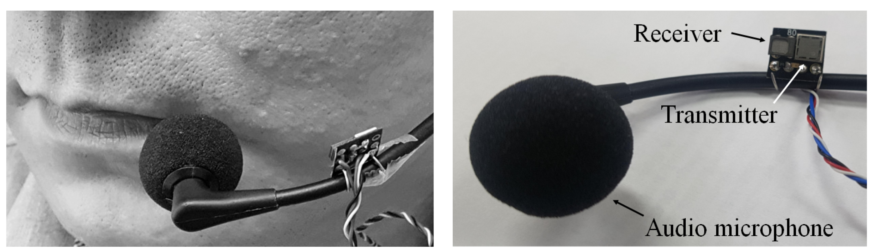
4.1. Experimental Setup

Two sensors were used to detect the ultrasonic Doppler shifts. One was attached to the wire frame of the headset microphone, and was used to detect Doppler shifts in the mouth and cheek area. The other was placed at the front of the throat for detection of Doppler sonar in the jaw and the neck area. Each sensor was composed of an ultrasonic transmitter emitting a continuous ultrasonic tone at 40 kHz and a wide band receiver that acquired signals that ranged from 10 to 65 kHz. An audio microphone was also used to simultaneously record audio-frequency range signals. The effective radiation area was 19.9 ${\mathrm{cm}}^2$, which was experimentally computed. Such an area proved to be sufficient to detect the subject’s articulatory movements. A photograph of the developed sensor mounted on a subject appears shown in Figure 4.

Five subjects participated in the recording, one female speaker and four male speakers whose ages ranged from 22 to 50. All subjects had no known articulatory problems. Newspaper articles were used as speaking materials. The properties of the dataset are summarized in

Table 3. Dataset properties.

Property	Value
Average number of utterances (per subject)	1062
Average duration of utterances (s)	6.44
Standard deviation of duration (s)	1.33
Maximum duration of utterance (s)	12.26
Minimum duration of utterance (s)	3.23
Average number of phonemes (per subject)	69,982

. The features were extracted from the windowed speech and from the windowed UDS. A 32 ms length for the Hanning window is commonly used to compute and extract the feature parameters at 16 ms intervals. The log-magnitude of the Fourier transform (FT) coefficients was used, and the length of the fast Fourier transform (FFT) was set at 256. Accordingly, the dimension of the log-power spectral feature vector was 128. The same FFT length was adopted to compute the UDS feature. Although the frequency resolution of the speech signal seemed relatively lower than other speech-related applications such as ASR, TTS, and speech coding, the experimental result showed that the performance of the DNN-based estimation was not improved with an increase in the length of the FFT.

The DNN was trained using 60% of the total features in the training stage, and the remaining features were used for validation (20%) and evaluation (20%). According to the results obtained by the validation dataset, the best performance was obtained when the DNN contained three hidden layers, and the number of the nodes in each hidden layer was set to $[1.5\times N_i]$. (where $\left[x\right]$ was the nearest integer value of x) $N_i$ was the number of input nodes, which was 160 (=16 features/channel × 2 channel × 5 frames). With the exception of the top layer, the sigmoid activation function was adopted. The momentum constant, $\alpha$, of the sigmoid active function was set to 0.7. A linear function was used in the top layer. The performance of the DNN was expected to improve with dropout regularization [44]. The experimental results also showed clear differences between when a dropout was adopted and when it was not, particularly for the test data. Hence, dropout regularization was adopted in the present study where a keep probability of 0.75 was employed.

Three objective measures were applied in the experiments, a Perceptual evaluation of the speech quality (PESQ) [37], the log-spectral distortion (LSD, in dB), and a short-time objective intelligibility measure (STOI) [45]. PESQ was calculated by comparing the reproduced speech with a sample of original reference speech, and it ranged from −0.5 to 4.5. The LSD of a speech signal is defined as

$$d_{LSD}=\frac{1}{N}\sum _{n=0}^{N-1}\sqrt{\frac{1}{P}\sum _{p=0}^{P-1}{\left[10·{log}_{10}\frac{|{\widehat{Y}}_{p,n}{|}^2}{|Y_{p,n}{|}^2}\right]}^2}$$

(21)

where $Y_{p,n}$ and ${\widehat{Y}}_{p,n}$ are the short-time Fourier transform (STFT) of the original speech and the reproduced speech, respectively, p is the frequency bin, n is an index of the time frame and N is the set of frames with speech presence. The STOI [45] was proposed as a correlation-based method to evaluate the speech intelligibility degradation caused by speech enhancement solutions. In the following section, all presented results were obtained from the evaluation data.

4.2. Determination of the Weights for Each Disturbance

We first investigated the performance of the predictor for the speech magnitude spectrum according to the weights for symmetrical and asymmetrical disturbances ($w_s$ and $w_a$ in (12)). This provided the necessary information for calculating the PD in future experiments. The number of the HE filter coefficients was set as 3, and the results appear in Figure 5. It was clear that the PESQs and STOIs had a decreasing trend as the weight of the asymmetrical disturbance increased. This was confirmed by the fact that the experimental correlation coefficients of the PESQs and STOIs with the asymmetrical weight values were −0.9286 and −0.9467, respectively. An asymmetrical disturbance was imposed on the PD so that negative differences would be perceived differently from positive ones due to masking effects [34]. The experimental results, however, showed that no remarkable benefit was gained by adopting an asymmetrical disturbance. This was somewhat different from previous studies that employed the PD metric [34,37].

The LSD revealed different trends by increasing the weights of the asymmetrical disturbance. A weak correlation (=0.5789) with asymmetrical disturbance was observed. The minimum for the LSD was obtained in cases where the weight of the asymmetrical disturbance was set as 0.2. The experimental results commonly indicate that a relatively small value of the asymmetrical disturbance would be helpful to improve the quality of the reproduced speech signals (higher PESQ, higher STOI and lower LSD). As a consequence, only symmetrical disturbance was used (e.g., $w_s=1,w_a=0$ in (12)) in the subsequent experiments.

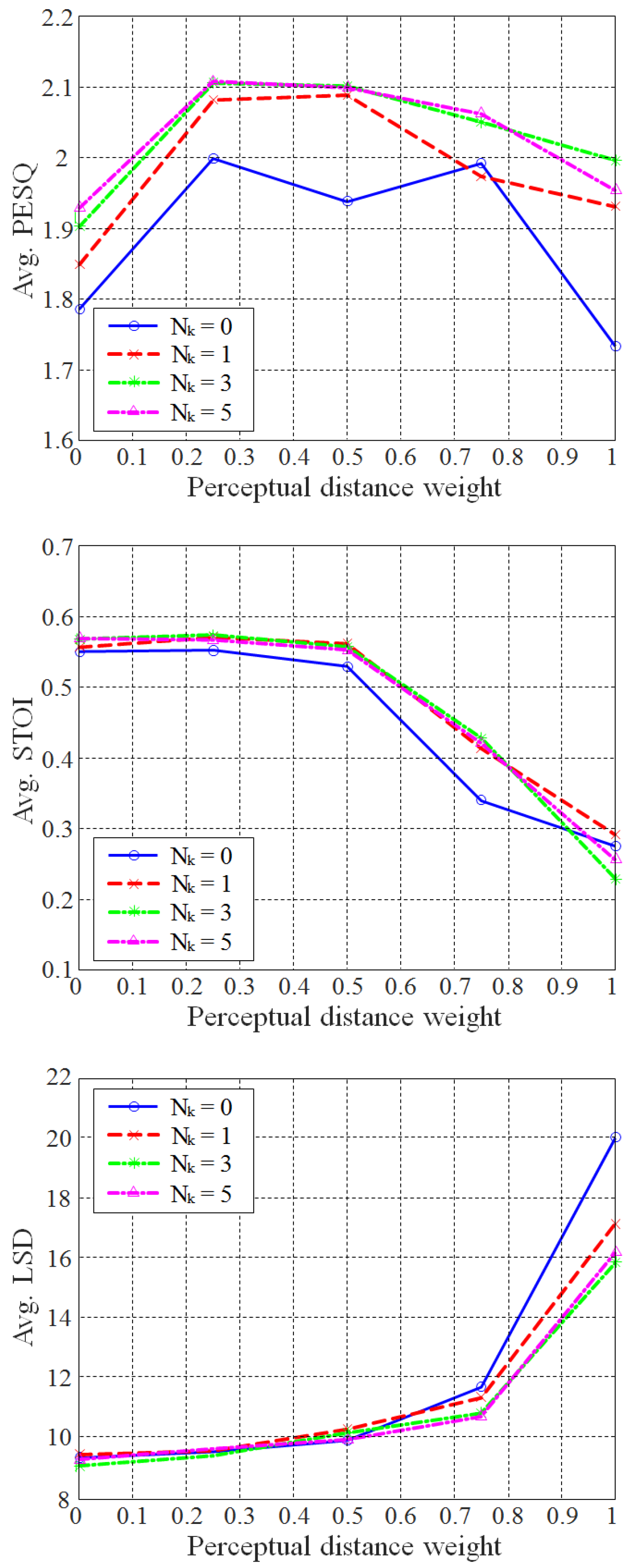
4.3. Objective Evaluation Results According to the PD Weights and the Length of the HE Filter

The various results were obtained by changing the weight for the PD term in (12), $w_s$, while the weight for the MSE was given by $w_M=1-w_s$. We also investigated how the objective performance was affected according to the length of the HE filter coefficients. Note that assigning zero to the weight of the PD term corresponds to the conventional MSE-based prediction rules. In a similar manner, a zero length for the HE filter meant that HE was not adopted in the SSI system, and, hence, the source signals were generated by white noise.

The results are presented in Figure 6 where $N_k$ denotes the length of the HE filter coefficients. A strong correlation (0.9551) between the average PESQ and $N_k$ was observed in the case of $w_s=0$. This means that the perceptual quality can be improved by applying HE even when the perceptual distance is not adopted. The PESQs were further increased by including the perceptual distance into the DNN loss function. In the case of $w_s=0.25$, maximum PESQs were obtained for all $N_k$. The average PESQ is also proportional to the length of the HE filter coefficients in this case ($\rho$ = 0.8109). And hence, the highest PESQ of 2.108 was achieved when $N_k$ and $w_s$ were set as 5 and 0.25, respectively. This was 0.11 higher than in the case of no HE. No further increase was observed when a weight greater than 0.5 was applied. This trend was common for HE filters of all lengths. When the relative weight for the PD term exceeded 0.5, the weight for the MSE term was less than 0.5. This resulted in excessive differences between the predicted spectra and the actual spectra, even though the resultant predicted spectra perceptually approximated the actual spectra. The testing of significance (two-way ANOVA) showed that the weight value was a major factor affecting the PESQ (p = 1.7 × 10${}^{-5}$) and an average Pearson correlation coefficient of 0.8191 was obtained between the PESQs and the weight values. That result indicated that the performance in terms of PESQ was remarkably improved by employing the PD in the objective function. However, excessive emphasis on the PD term in the objective function actually degraded the PESQ, as shown in the PESQ values for $w_s>0.5$. This means that improvements in PESQ can be accomplished by not only considering the MSE but the PD as well.

There was a clear relationship between the STOIs and the perceptual weights, as shown in the middle of Figure 6. The average STOI values take the form of decreasing curves with increases in the weights of the perceptual distance. Unlike the PESQ, the STOIs are not remarkably changed by the length of the HE filter coefficients (p = 0.2302, $\rho$ = 0.4060). The average STOIs were significantly varied according to the PD weight. The p-value of the $w_s$ factor was 4.61 × 10${}^{-10}$ and the Pearson correlation coefficient of the STOI with the $w_s$ was −0.8930. This indicated that the weight for the PD was the key factor affecting STOI. It is noteworthy that the maximum STOIs among all perceptual distance weights are obtained at $w_s=0.25$, which is same as in the case of the PESQ.

The average correlation between the LSD and the value of the PD weight was 0.8365. This indicates that the LSD takes the form of increasing curves with increases in the PD weight. This result was somewhat expected, because LSD is closely related to MSE. Increasing the weight of the PD means lowering the MSE weight, which results in a larger spectral distortion. Based on the combined results of the PESQ and LSD, it can be inferred that lowering the LSD is not a necessary condition for obtaining high-quality reproduced speech. For example, setting the PD weight as 0.0 yielded the lowest LSD for all $N_k$. In this case, however, the lower PESQs (≤2.0) were obtained, regardless of $N_k$. This means that for a reasonable level of LSD (e.g., ≤12 dB, as shown in Figure 6), the DNN-based predictor of PD yielded perceptually preferred results. However, an excessively large LSD (e.g., ≥12 dB) leads to a decrease in the perceptual quality of the reproduced speech signals. Such a result was typically observed in the case of $N_k=0$, as shown at the top of Figure 6 (average PESQ).

4.4. Comparison with Other Methods

One of the objectives of the present study is to improve the quality of the reproduced speech signals by maintaining a harmonic structure in the voiced segments. A degree of harmonicity can be measured by the autocorrelation function, which is computed in the time domain. In this study, the average autocorrelation value over the voiced frames was also adopted to evaluate the quality of the reproduced speech signals. The average autocorrelation of the speech samples $y\left(0\right),\cdots ,y(N-1)$ is given by

$${\overline{R}}_{yy}=\frac{1}{N_v}\sum _{k=1}^{N_f}w\left(k\right)\left[\frac{1}{W_L}\sum _{n=1}^{W_L}y(k{W}_R+n)y(k{W}_R+n-P_k)\right]$$

(22)

where $N_v$, $N_f$, $W_L$, and $W_R$ denote the number of the voiced frames, the total number of frames, the frame length, and the frame interval, respectively. $w\left(k\right)$ is given by

$$w\left(k\right)=\left\{\begin{array}{cc}1\hfill & \mathrm{if} k-\mathrm{th} \mathrm{frame} \mathrm{is} \mathrm{voiced} \mathrm{frame}.\hfill \\ 0\hfill & \mathrm{otherwise}.\hfill \end{array}\right.$$

(23)

$P_k$ is the pitch period for the k-th frame that is estimated by the speech signal. For the speech signal, the average of ${\overline{R}}_{yy}$ was obtained as 0.881. This indicates that voiced speech samples are strongly correlated at pitch intervals.

The performance of the proposed method was compared with other methods that were designed for estimating speech parameters. The list of the methods for comparison is shown in

Table 4. Performance comparison of the test set for the different estimation methods.

Method	Avg. PESQ	Avg. STOI	Avg. LSD	Avg. R
Linear regression (LR)	1.515	0.424	9.700	0.114
Multivariate linear regression (MLR)	1.551	0.469	9.105	0.135
Gaussian mixture model (GMM)	1.535	0.472	9.484	0.109
Recurrent neural networks (RNN)	1.648	0.538	8.306	0.133
Long short term memory (LSTM)	1.684	0.556	8.063	0.159
Multi-layer perceptron (MLP)	1.786	0.551	9.300	0.160
Multi-layer perceptron (MLP) with PD	1.999	0.553	9.503	0.211
Multi-layer perceptron (MLP) with PD + HE	2.108	0.567	9.590	0.402

. These methods were already employed in SSI (e.g., Gaussian mixture model (GMM) [16,21,22,25,26,27,30], long short term memory (LSTM) [27,46], and multi-layer perceptron (MLP) [10,24,25,27]). For the methods RNN, LSTM, and MLP (without HE), the hyperparameters were tuned to minimize the overall costs. The resultant architecture of the RNN and LSTM consisted of three hidden layers, 160 hidden nodes, and four time steps. The same dataset was commonly used for all methods to obtain the results.

The results are presented in Table 4. The superiority of the proposed method (MLP with PD and HE) is remarkable in terms of the average PESQ and STOI. The MLP + PD + HE is the only method that produces an average PESQ greater than 2.0. The common property of the methods LR, MLR, GMM is that speech parameters are given by a linear combination of some representative vectors (e.g., mean vectors of each Gaussian component). This resulted in ambiguous and unclear voices, due to the averaging effects. These are the possible reasons for lowering the PESQ and STOI. Such problems were partially alleviated by applying the neural networks (RNN, LSTM, MLP), and hence the average PESQ and STOI were increased. The quality of the reproduced speech signals was further improved by applying PD. The average LSD, however, was increased in the case where the PD was adopted. This is due to the fact that the loss function of the MLP + PD method is given by the weighted sum of the two costs (MSE and PD), resulting in increasing MSE compared with RNN, LSTM, and MLP methods. Although the average LSDs of the PD-based methods are greater than those of other methods, perceptually more preferred results can be achieved by the PD-based methods. This is confirmed by the fact that the two PD-based methods (MLP + PD and MLP + PD + HE) yielded a higher average PESQ, compared with other methods.

The feasibility of harmonic enhancement (HE) is also confirmed by the results shown in Table 4. The average PESQ and STOI of the MLP + PD + HE method are 2.108 and 0.567, which are the highest among all methods. The average PESQ was increased by 0.107 when HE was adopted. Such improvements in terms of PESQ are due mostly to the preservation of a harmonic structure in the voiced segments. This is also confirmed by the autocorrelation results where the MLP + PD + HE method revealed a remarkably high value compared with other methods. Although the maximum of the average autocorrelation obtained from the reproduced speech signals is almost half that from the voiced speech signals, this was sufficient to increase the average PESQ. The Pearson correlation between the averages for PESQ and autocorrelation is 0.8857, which is the highest among other evaluation metrics (0.7783 and 0.2237 for average STOI and LSD, respectively). This indicates that enhancement of a harmonic structure in the voiced regions sufficiently contributes to increasing the overall PESQs.

The spectra of each reproduced speech signal were visually inspected to verify the effectiveness of the proposed method in terms of maintaining a harmonic structure in the voiced regions. An example of the spectra of the original speech, reproduced speech by the baseline method, and reproduced speech by the proposed method appears in Figure 7. Note that the PD and the HE filter were not adopted in the baseline method, whereas the 3-tab HE filter and an objective function with PD ($w_s$ = 0.25) were adopted in the proposed method. In this example, the selected speech segment corresponded to the typical voiced region in which a harmonic structure was apparent, as shown at the top of Figure 7. Compared with the baseline method ($w_s$ = 0.0 and $N_k$ = 0), the proposed method revealed a clearer harmonic structure. Such a pattern was evident in the relatively low frequency regions (≤1.5 kHz in this example), because the human auditory system is most sensitive to signals in the vicinity of 1 kHz, and the DNN was trained to further reduce errors within this band. In the baseline method, however, the human auditory system and HE were not taken into consideration in training the DNN, which resulted in a very weak harmonic structure even for the voiced regions. Also, the amplitudes of the low band harmonics (≤800 Hz in this example) were excessively higher than that of other harmonics. This has been a major cause of the tonal noise that is often perceived in reproduced speech.

In conclusion, the problems associated with a loss of harmonic structure that are frequently encountered when using conventional SSI methods were partially alleviated by adopting PD and HE. Problems persisted with the proposed method, however, where the amplitude of each harmonic was either over- or under-emphasized.

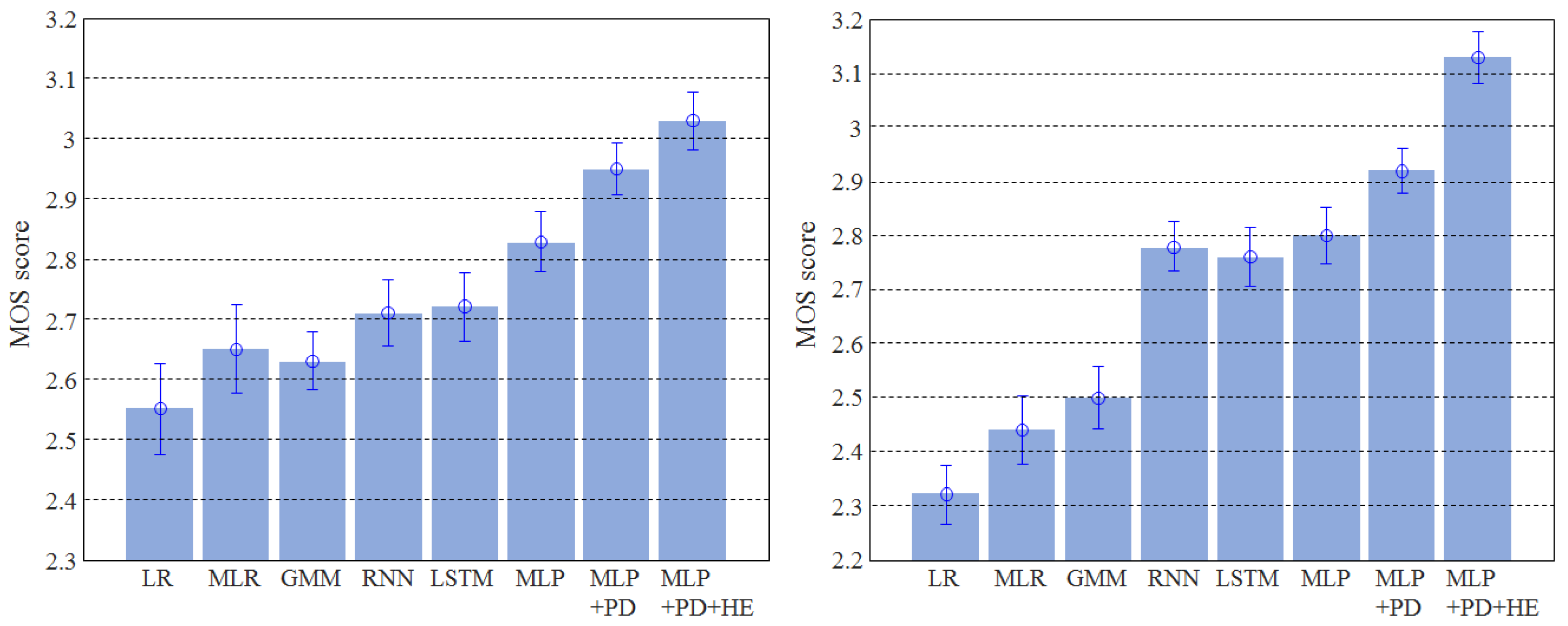
4.5. Subjective Evaluation

An informal listening test was conducted to evaluate the subjective quality of reproduced speech signals using the Mean Opinion Score (MOS) test. In this test, 20 listeners with normal hearing ability participated and were asked to subjectively score the quality of the reproduced speech signals in terms of intelligibility and naturalness. The quality rating scale for each factor is Excellent = 5/Good = 4/Fair = 3/Poor = 2/Bad = 1. The data set for evaluation was composed of a randomly selected 20 pairs of utterances. Quality evaluation was carried out on the speech signals reproduced by the eight schemes presented in Table 4. Note that in the MLP-based methods with the PD and HE, $w_s$ and $N_k$ were chosen so that the average PESQ was maximized according to the objective results. The order of the stimuli synthesized by each method was randomly permuted. Each subject was allowed to listen to the stimuli as many times as needed before decision. The test stimuli were presented through a headphone in a quiet room.

The results in Figure 8 show the average MOSs for each method. Similar to the results of PESQ, the highest MOS was obtained by the approach using both MSE and PD with HE (MLP + PD + HE). The maximum MOS scores were obtained by the proposed method (MMP + PD + HE) both in terms of intelligibility and naturalness. Only the MLP + PD + HE method yielded an average MOS score greater than 3.0. The listeners also indicated that both intelligibility and naturalness were superior to the other methods. In terms of naturalness, the relatively low MOS scores of the three linear estimation-based methods (LR, MLR, and GMM) are mainly due to the averaging effects of the estimation scheme, which resulted in ambiguous and unclear voices. The quality improvements were achieved in part, by applying the NN-based methods. Applying the PD and HE further improved the quality of the reproduced speech signals. The listeners indicated the speech signals synthesized by the MLP + PD + HE method were clearer and more natural than other methods. A possible explanation for such MOS improvements over the conventional DNN-based methods is that a certain degree of harmonic structure is maintained in the voiced regions of the synthesized speech signals.

The listeners also indicated that the proposed SSI method yielded noisy speech, although the overall quality was improved over the baseline method (in case of $w_s=0$, $N_k=0$). This was due mainly to the usage of a random phase in the synthesizing procedure. But the reproduced speech signals continued to sound noisy when a least square-based phase estimation method [43] was adopted. Accordingly, it is highly desirable to apply a more reliable phase estimation scheme to construct the prediction rules for speech parameters.

5. Conclusions

Conventional SSI methods suffer from a deficiency in the estimation of spectrum details, which often results in a degradation of the quality of reproduced speech signals. In the SSI system presented herein, research efforts were dedicated not only to estimating the spectral envelope, but also to preserving the harmonic structure, particularly for the voiced regions of speech. To this end, harmonic enhancement was employed. This was different from the previous method with harmonic enhancement in that the coefficients of the harmonic enhancement filter were arranged in a manner that would minimize the distance from the original speech. The whole spectrum was obtained through a DNN, which was trained to minimize the distance. Another unique aspect of the proposed method is the adoption of an objective function that includes both MSE and perceptual distance. The perceptual distance was computed similar to the method used to calculate the PESQ.

The effectiveness of the proposed method was confirmed in experiments, which generated both objective and subjective results that were superior to those of previous methods. There is room, however, for further improvement. For example, the pitch period used for harmonic enhancement was estimated using an open-loop optimization framework. Since the quality of the reproduced speech is more important than the accuracy of pitch estimation, a closed loop optimization method that iteratively minimizes the perceptual difference between actual speech signals and those that are reproduced would be helpful in improving the quality of the synthesized speech signals. Our future studies will focus on these issues.

References

1. Denby, B.; Schultz, T.; Honda, K.; Hueber, T.; Gilbert, J.M.; Brumberg, J.S. Silent speech interfaces. Speech Commun. 2010, 4, 270–287. [Google Scholar] [CrossRef] [Green Version]
2. Schultz, T.; Wand, M.; Hueber, T.; Krusienski, J.; Herff, C.; Brumberg, J. Biosignal-based spoken communication: A survey. IEEE/ACM Trans. Audio Speech Lang. Process. 2017, 12, 2257–2271. [Google Scholar] [CrossRef]
3. Quatieri, T.F.; Brady, K.; Messing, D.; Campbell, J.P.; Campbell, W.M.; Brandstein, M.S.; Weinstein, C.J.; Tardelli, J.D.; Gatewood, P.D. Exploiting nonacoustic sensors for speech encoding. IEEE Trans. Audio Speech Lang. Process. 2006, 2, 533–544. [Google Scholar] [CrossRef]
4. Jiao, M.; Lu, G.; Jing, X.; Li, S.; Li, Y.; Wang, J. A novel radar sensor for the non-contact detection of speech signals. Sensors 2010, 10, 4622–4633. [Google Scholar] [CrossRef] [PubMed] [Green Version]
5. Li, S.; Wang, J.-Q.; Niu, M.; Liu, T.; Jing, X.-J. The enhancement of millimeter wave conduct speech based on perceptual weighting. Prog. Electromagn. Res. B 2008, 9, 199–214. [Google Scholar] [CrossRef] [Green Version]
6. Li, S.; Tian, Y.; Lu, G.; Zhang, Y.; Lv, H.; Yu, X.; Xue, H.; Zhang, H.; Wang, J.; Jing, X. A 94-GHz milimeter-wave sensor for speech signal acquisition. Sensors 2013, 13, 14248–14260. [Google Scholar] [CrossRef]
7. Li, S.; Tian, Y.; Lu, G.; Zhang, Y.; Xue, H.; Wang, J.; Jing, X. A new kind of non-acoustic speech acquisition method based on millimeter wave radar. Prog. Electromagn. Res. B 2012, 130, 17–40. [Google Scholar] [CrossRef] [Green Version]
8. Lin, C.-S.; Chang, S.-F.; Chang, C.-C.; Lin, C.-C. Microwave human vocal vibration signal detection based on Doppler radar technology. IEEE Trans. Microw. Theory Technol. 2010, 8, 2299–2306. [Google Scholar] [CrossRef]
9. Denby, B.; Stone, M. Speech synthesis from real time ultrasound images of the tongue. In Proceedings of the IEEE International Conference on Acoustics, Speech and Signal Processing, Montreal, QC, Canada, 17–21 May 2004; pp. 685–688. [Google Scholar]
10. Denby, B.; Qussar, Y.; Dreyfus, G.; Stone, M. Prospects for a silent speech interface using ultrasound imaging. In Proceedings of the IEEE International Conference on Acoustic Speech Signal Processing, Toulouse, France, 14–19 May 2006; pp. 365–368. [Google Scholar]
11. Hueber, T.; Aversano, G.; Chollet, G.; Stone, M. Eigentongue feature extraction for an ultrasound-based silent speech interface. In Proceedings of the IEEE International Conference on Acoustics, Speech and Signal Processing, Honolulu, HI, USA, 15–20 April 2007; pp. 1245–1248. [Google Scholar]
12. Cornu, T.L.; Milner, B. Generating intelligible audio speech from visual speech. IEEE Trans. Audio Speech Lang. Process. 2017, 9, 1447–1457. [Google Scholar] [CrossRef] [Green Version]
13. Deligne, S.; Potamianos, G.C.; Neti, C. Audio-visual speech enhancement with AVCDCN (Audio-Visual Codebook Dependent Cepstral Normalization). In Proceedings of the International Conference on Spoken Language Processing, Denver, CO, USA, 16–20 September 2002; pp. 1449–1452. [Google Scholar]
14. Girin, L.; Varin, L.; Feng, G.; Schwartz, J.L. Audiovisual speech enhancement: New advances using multi-layer perceptrons. In Proceedings of the IEEE 2nd Workshop on Multimedia Signal Processing, Redondo Beach, CA, USA, 7–9 December 1998; pp. 77–82. [Google Scholar]
15. Potamianos, G.; Neti, C.; Gravier, G.; Garg, A.; Senior, A.W. Recent advances in the automatic recognition of audiovisual speech. Proc. IEEE 2003, 9, 1306–1326. [Google Scholar] [CrossRef]
16. Almajai, T.B.; Milner, B. Visually derived Wiener filters for speech enhancement. IEEE Trans. Audio Speech Lang. Process. 2011, 6, 1642–1651. [Google Scholar] [CrossRef]
17. Kalgaonkar, K.; Raj, B. Ultrasonic doppler sensor for speaker recognition. In Proceedings of the IEEE International Conference on Acoustics, Speech and Signal Processing, Las Vegas, NA, USA, 30 March–4 April 2008; pp. 4865–4868. [Google Scholar]
18. Lee, K.-S. Speech enhancement using ultrasonic doppler sonar. Speech Commun. 2019, 110, 21–32. [Google Scholar] [CrossRef]
19. Lee, K.-S. Silent speech interface using Doppler sonar. IEICE Trans. Inf. Syst. 2020, 8, 1875–1887. [Google Scholar] [CrossRef]
20. Raj, B.; Kalgaonkar, K.; Harrison, C.; Dietz, P. Ultrasonic doppler sensing in HCI. IEEE Pervasive Comput. 2012, 2, 24–29. [Google Scholar] [CrossRef]
21. Toth, A.R.; Raj, B.; Kalgaonkar, K.; Ezzat, T. Synthesizing speech from doppler signals. In Proceedings of the IEEE International Conference on Acoustics, Speech and Signal Processing, Dallas, TX, USA, 14–19 March 2010; pp. 4638–4641. [Google Scholar]
22. Toda, T.; Shikano, K. NAM-to-Speech conversion with Gaussian Mixture Models. In Proceedings of the Interspeech, Lisbon, Portugal, 4–8 September 2005; pp. 1957–1960. [Google Scholar]
23. Toda, T.; Nakagiri, M.; Shikano, K. Statistical voice conversion techniques for body-conducted unvoiced speech enhancement. IEEE Trans. Audio Speech Lang. Process. 2012, 9, 2505–2517. [Google Scholar] [CrossRef]
24. Diener, L.; Janke, M.; Schultz, T. Direct conversion from facial myoelectric signals to speech using deep neural networks. In Proceedings of the International Joint Conference on Neural Networks, Killarney, Ireland, 12–17 July 2015; pp. 1–7. [Google Scholar]
25. Hueber, T.; Bailly, G. Statistical conversion of silent articulation into audible speech using full-covariance HMM. Comput. Speech Lang. 2016, 36, 274–293. [Google Scholar] [CrossRef]
26. Janke, M.; Wand, M.; Nakamura, K.; Schultz, T. Further investigations on EMG-to-speech conversion. In Proceedings of the IEEE International Conference on Acoustics, Speech and Signal Processing, Kyoto, Japan, 25–30 March 2012; pp. 365–368. [Google Scholar]
27. Janke, M.; Diener, D. EMG-to-Speech: Direct generation of speech from facial electromyographic signals. IEEE Trans. Audio Speech Lang. Process. 2017, 12, 2375–2385. [Google Scholar] [CrossRef] [Green Version]
28. Lee, K.-S. EMG-based speech recognition using Hidden Markov Models with global control variables. IEEE Trans. Biomed. Eng. 2008, 3, 930–940. [Google Scholar] [CrossRef]
29. Lee, K.-S. Prediction of acoustic feature parameters using myoelectric signals. IEEE Trans. Biomed. Eng. 2010, 7, 1587–1595. [Google Scholar]
30. Toth, A.R.; Wand, M.; Schultz, T. Synthesizing speech from electromyography using voice transformation techniques. In Proceedings of the Interspeech, Brighton, UK, 6–10 September 2009; pp. 652–655. [Google Scholar]
31. Wand, M.; Janke, M.; Schultz, T. Tackling speaking mode varieties in EMG-based speech recognition. IEEE Trans. Biomed. Eng. 2014, 10, 2515–2526. [Google Scholar] [CrossRef]
32. Rabiner, L.R.; Juang, B.-H. Auditory-based spectral analysis models. In Fundamentals of Speech Recognition; Prentice Hall: Englewood Cliffs, NJ, USA, 1993; pp. 132–139. [Google Scholar]
33. Cernak, M.; Asaei, A.; Hyafil, A. Cognitive Speech Coding: Examining the Impact of Cognitive Speech Processing on Speech Compression. IEEE Signal Process. Mag. 2018, 3, 97–109. [Google Scholar] [CrossRef]
34. Martin, J.M.; Gomez, A.M.; Gonzalez, J.A.; Peinado, A.M. A deep learning loss function based on the perceptual evaluation of the speech quality. IEEE Signal Process. 2018, 11, 1680–1684. [Google Scholar] [CrossRef]
35. Moritz, N.; Anemu¨ller, J.B.; Kollmeier, B. An Auditory Inspired Amplitude Modulation Filter Bank for Robust Feature Extraction in Automatic Speech Recognition. IEEE Trans. Audio Speech Lang. Process. 2015, 11, 1926–1937. [Google Scholar] [CrossRef]
36. Tachibana, K.; Toda, T.; Shiga, Y.; Kawai, H. An Investigation of Noise Shaping with Perceptual Weighting for Wavenet-Based Speech Generation. In Proceedings of the IEEE International Conference on Acoustics, Speech and Signal Processing, Calgary, AB, Canada, 15–20 April 2018; pp. 5664–5668. [Google Scholar]
37. ITU-T, Rec. P. 862; Perceptual Evaluation of Speech Quality (PESQ): An Objective Method for End-to-End Speech Quality Assessment of Narrow Band Telephone Networks and Speech Codecs. International Telecommunication Union-Telecommunication Standardisation Sector: Geneva, Switzerland, 2001.
38. Nakamura, K.; Janke, M.; Wand, M.; Schultz, T. Estimation of fundamental frequency from surface electromyographic data:EMG-to-F0. In Proceedings of the IEEE International Conference on Acoustics, Speech and Signal Processing, Prague, Czech Republic, 22–27 May 2011; pp. 573–576. [Google Scholar]
39. Xu, Y.; Du, J.; Dai, L.-R.; Lee, C.-H. A regression approach to speech enhancement based on deep neural networks. IEEE Trans. Audio Speech Lang. Process. 2015, 1, 7–19. [Google Scholar] [CrossRef]
40. Jin, W.; Liu, X.; Scordilis, M.S.; Han, L. Speech enhancement using harmonic emphasis and adaptive comb filtering. IEEE Trans. Audio Speech Lang. Process. 2010, 2, 356–368. [Google Scholar] [CrossRef]
41. Han, K.; Wang, D. Neural network based pitch tracking in very noisy speech. IEEE Trans. Audio Speech Lang. Process. 2014, 12, 2158–2168. [Google Scholar] [CrossRef]
42. Kato, A.; Kinnunen, T.H. Statistical Regression Models for Noise Robust F0 Estimation Using Recurrent Deep Neural Networks. IEEE/ACM Trans. Audio Speech Lang. Process 2019, 12, 2336–2349. [Google Scholar] [CrossRef]
43. Griffin, D.W.; Lim, J.S. Signal estimation from the modified short-time fourier transform. IEEE Trans. Acoust. Speech Signal Process. 1984, 32, 236–243. [Google Scholar] [CrossRef]
44. Hinton, G.E. Training products of experts by minimizing contrastive divergence. Neural Comput. 2002, 8, 1711–1800. [Google Scholar] [CrossRef]
45. Taal, C.H.; Hendriks, R.C.; Heusdens, R.; Jensen, J. An algorithm for intelligibility prediction of time-frequency weighted noisy speech. IEEE/ACM Trans. Audio Speech Lang. Process. 2011, 7, 2125–2136. [Google Scholar] [CrossRef]
46. Yadav, R.; Sardana, A.; Namboodiri, V.P.; Hegde, R.M. Speech prediction in silent videos using variational autoencoders. In Proceedings of the IEEE International Conference on Acoustics, Speech and Signal Processing, Totonto, ON, Canada, 6–11 June 2021; pp. 7048–7052. [Google Scholar]
Figure 1. Block diagram of the baseline ultrasonic SSI system. (Top): Training procedure. (Bottom): Synthesis procedure.
Applsci 12 00827 g001
Figure 2. Examples of original (bold line) and the predicted (dotted line) speech spectra.
Applsci 12 00827 g002
Figure 3. Block diagram of the proposed ultrasonic SSI system.
Applsci 12 00827 g003
Figure 4. Photograph of the ultrasonic sensors. (Left): Mounted on the right cheek. (Right): Magnified sensor portion.
Applsci 12 00827 g004
Figure 5. Objective evaluation results according to the weights of the asymmetrical disturbance. (Top): Average PESQs. (Middle): STOIs. (Bottom): LSDs.
Applsci 12 00827 g005
Figure 6. Objective evaluation results for the various perceptual distance weights and the taps of the HE filters ( N k ). (Top): Average PESQs. (Middle): STOIs. (Bottom): LSDs.
Applsci 12 00827 g006
Figure 7. Example of spectra. (Top): Original speech. (Middle): Predicted using baseline method ( w s = 0 , N k = 0 ). (Bottom): Predicted using PD and He ( w s = 0.25 , N k = 3 ).
Applsci 12 00827 g007
Figure 8. Average MOS scores with error bars for each method. (Left): Intelligibility. (Right): Naturalness.
Applsci 12 00827 g008