Complex Variable Solution for Stress and Displacement of Layered Soil with Finite Thickness

Abstract

The static problem of a layered isotropic elastic body is a very useful research subject in relation to the analysis and design of foundation works. Due to the complexity of the problem, there is no analytical solution to the problem so far. This study provides an efficient analytical approach to accurately calculate the displacement and stress fields of the soil. The constraints of bedrock on soil, different soil layer thickness and the shear stress of the foundation on soil were all taken into account in the analysis. In this study, each layer is regarded as an isotropic elastomer with infinite width, and the layers are in complete contact. By using conformal mapping, each layer is mapped to a unit circle, and the two complex potential functions are expanded into Taylor series with unknown coefficients. These unknown coefficients are obtained by satisfying boundary conditions and continuity conditions. The boundary and continuity conditions were verified in this paper. As a validation step, we compared the analytical results for the settlement with the results of the ANSYS numerical simulations and found good agreement. Parametric analyses were also carried out to investigate the influence of different distribution forms of base pressure on surface settlement, and the effects of layered properties on the surface settlement and stress field.

1. Introduction

In many places, it is common to see compressible soil overlying rigid bedrock. In this case, the stress and displacement of soil are obviously different from that of a semi-infinite body medium [1]. Natural soils tend to be horizontally layered during deposition, the density and hardness of each layer are generally different, and the deformation characteristics may vary greatly [2]. When the stress in the soil is too large, the deformation of the soil will cause unacceptable settlement of the building and even the instability of the entire soil. Therefore, an accurate calculation of soil stress and displacement is an important basis for the stability analysis of building foundations and geotechnical structures [3].

Finite element method can provide useful solutions to many complex geological conditions. However, extensive computational time is required, especially when complete parametric analyses need to be performed [4]. Analytical solutions provide an efficient and quick approach to gain insight into the nature of the problem [5]; in addition, they enable analyses of a wide range of parameter values so that the physics of the problem can be better understood [4]. In the past, researchers mainly used the integral transformation method to analyze the elastic static problems of layered soil. Burmister [6] provided the integral expression of stress and displacement of two layers of soil under a flexible circular foundation based on the integral transformation method, and also established an empirical formula for surface settlement when both layers of soil consist of incompressible materials. In many studies in the literature, the soil surface is subjected to a circular uniformly distributed load, which is considered a spatial axisymmetric problem. Both layers of soil are linear elastomers and in complete contact. The second layer of soil was infinitely deep. Then, smooth contact [7] and three-layer [8] soil with complete contact were considered. Because only the integral transformation equations of stress and displacement could be derived by the integral transformation method, many numerical methods were proposed to solve the integral equations. Barovich et al. [9] studied the stress field of two-layer elastomer under elliptical distributed load, in which the second-layer elastomer was a semi-infinite body, and presented a numerical value of the stress on the axis of symmetry. Chen [10] identified the shortcomings of this method, that is, the integral converges slowly or does not even converge at the boundary. Chen [10] improved the method to solve the problem of the stress field and displacement field of three-layer soil under circular and rectangular loads. However, the subsoil was still semi-infinite, which means this method was not suitable for bedrock at the bottom of the soil. Since then, many scholars have used the integral transformation method to study the layered material problem, but the bottom layer was assumed to be a semi-infinite body [11,12,13,14,15,16,17,18,19,20,21,22,23,24,25,26,27,28].

When there is bedrock under the soil, it is very difficult to obtain an analytical solution regarding the stress and displacement due to the constraint of the bedrock on the soil. At present, only Lu et al. [1] have obtained an explicit analytical expression for the stress and displacement of single-layer finite thickness soil under the action of a strip foundation by a complex variable method. In this paper, the solution in [1] is extended to layered soil, and the complex variable method [29] is used to solve the stress and displacement of multi-layer soil above bedrock under the action of a strip shallow foundation. Under the action of a strip foundation, the soil is subjected to a strip-distributed load. It is assumed that the distributed load does not change along the direction perpendicular to the surface; thus, the problem solved in this paper is a plane strain problem [1]. In this paper, each layer of soil is regarded as an isotropic linear elastic body with finite thickness, and the layers are in complete contact with each other. Each layer of soil is mapped into a unit circle by using a conformal transformation tool in the complex variable method, and the two complex potential functions of each layer of soil can be expanded into a Taylor series. According to the stress boundary condition of the surface, the displacement boundary condition of the soil bottom, and the stress and displacement continuity conditions on the contact surface, the equation for solving the complex potential function coefficients can be obtained, and through the complex potential function, the exact solution for the stress and displacement at any point in the soil can be obtained. Differently to the integral transformation method, for any given load, this method can directly provide an explicit expression of the stress and displacement in each layer of soil. At the same time, the corresponding FORTRAN program compiled in this paper is characterized by fast calculation speed and high calculation accuracy, which are of great benefit to engineering applications.

2. Problem Statement and Method Presentation

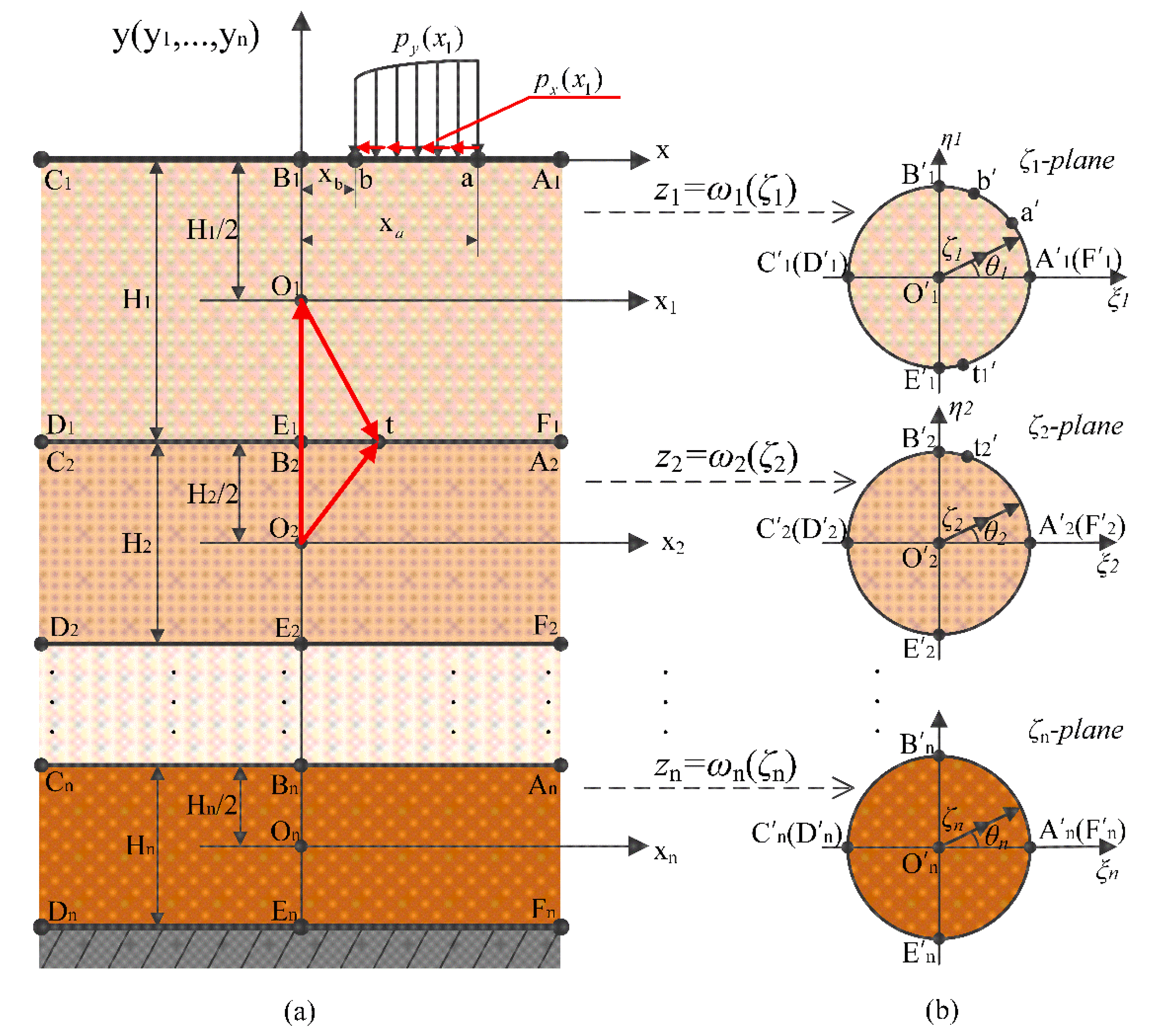
This paper deals with the case of complete contact between layers of multi-layer soil and complete constraint with bedrock below it. When the soil surface is subjected to distributed load, the deformation of bedrock is considered to be negligible compared with the deformation of soil, that is, the displacement component on the interface between the soil and bedrock is equal to zero. Figure 1a shows a problem in which the upper boundary is the stress boundary condition, the lower boundary is the displacement boundary condition, and the contact surface of each layer is the stress and displacement continuity condition.

In Figure 1a, the four end points ($\mathrm{A},\mathrm{C},\mathrm{D},\mathrm{F}$) of each layer of soil are points at infinity. $t$ is any point on the contact surface. There is a vector relation about$t$:

$$\overrightarrow{O_2{O}_1}+\overrightarrow{O_{1}t}=\overrightarrow{O_{2}t}$$

(1)

As shown in Figure 1, the j-th layer (j = 1,2,⋯,n) soil is mapped to the inner domain of the unit circle in the ζ_j plane. The mapping function is:

$$z_j={\omega }_j\left({\zeta }_j\right)=\frac{H_j}{\pi }\ln \left(\frac{1+{\zeta }_j}{1-{\zeta }_j}\right)$$

(2)

where $z_j$ is any point in the j-th layer soil, $z_j=x_j+i{y}_j$, $i=\sqrt{-1}$; $H_j$ is the thickness of the j-th layer soil. ζ_j is the point where $z_j$ maps to the image plane. ζ_j =${\rho }_{\mathrm{j}}{\mathrm{e}}^{i{\theta }_{\mathrm{j}}}$, ${\rho }_j=1$ corresponds to the upper and lower boundaries in the j-th layer soil, and ${\sigma }_j$ is used to denote ζ_j at this time.

As shown in Figure 1, in the ζ₁ plane, the circumference of the unit circle (│${\sigma }_1$│ = 1) corresponds to the upper and lower boundaries of the first layer of soil. ${\mathrm{A}}_1$, ${\mathrm{B}}_1$, ${\mathrm{C}}_1$, ${\mathrm{D}}_1$, ${\mathrm{E}}_1$, ${\mathrm{F}}_1$ are mapped to ${\mathrm{A}}_1^{\prime }$, ${\mathrm{B}}_1^{\prime }$, ${\mathrm{C}}_1^{\prime }$, ${\mathrm{D}}_1^{\prime }$, ${\mathrm{E}}_1^{\prime }$, ${\mathrm{F}}_1^{\prime }$, respectively. The upper boundary ($\overline{A_1{\mathrm{B}}_1{\mathrm{C}}_1}$) is mapped to the upper semicircle ($\stackrel{⌢}{A_1^{\prime }{B}_1^{\prime }{C}_1^{\prime }}$). The lower boundary ($\overline{{\mathrm{D}}_1{\mathrm{E}}_1{\mathrm{F}}_1}$) is mapped to the lower semicircle ($\stackrel{⌢}{D_1^{\prime }{E}_1^{\prime }{F}_1^{\prime }}$). The coordinate origin (${\mathrm{O}}_1$) is mapped to the center of the unit circle (${\mathrm{O}}_1^{\prime }$) of the ζ₁ plane. On the upper and lower boundaries, all points of $x_1\to +\infty$ are mapped to the same point (${\sigma }_1$ = 1) of the ζ₁ plane, and all points of $x_1\to -\infty$ are mapped to the same point (${\mathsf{\sigma }}_1$ = −1) of the ζ₁ plane. The coordinate axes $x_1$ and $y_1$ are mapped to ${\xi }_1$ and ${\eta }_1$ axes. The points $a$ and $b$ are mapped to $a^{\prime }$ and $b^{\prime }$. The rest of the layers can be deduced by analogy.

By substituting Equation (2) into Equation (1), the relationship between ${\theta }_1$ and ${\theta }_2$ at the same point $t$ on the contact surface of the 1st layer and the 2nd layer can be obtained:

$${\theta }_2=\arccos \left(\frac{T_1{}^2-1}{T_1{}^2+1}\right)$$

(3)

where $T_1={\left(-sin{\theta }_1/\left(1-cos{\theta }_1\right)\right)}^{H_1/H_2}$.

In the same way, on the contact surface of the j-th layer and the j + 1-th layer:

$${\theta }_{j+1}=\arccos \left(\frac{T_j{}^2-1}{T_j{}^2+1}\right)$$

(4)

where $T_{j+1}={\left(-sin{\theta }_j/\left(1-cos{\theta }_j\right)\right)}^{H_j/H_{j+1}}$, $j=1,2,\dots ,n-1$.

${\sigma }_{j,x}$, ${\sigma }_{j,y}$ and ${\tau }_{j,xy}$ are the horizontal normal stress, vertical normal stress and shear stress of the j-th layer soil, respectively, and $u_j$ and $v_j$ are the horizontal displacement and vertical displacement of the j-th layer soil, respectively. The three stress components ${\sigma }_{j,x}$, ${\sigma }_{j,y}$, ${\tau }_{j,xy}$ and two displacement components $u_j$, $v_j$ of point $z_j$ can be expressed as [21]:

$$\{\begin{array}{l}{\sigma }_{j,x}+{\sigma }_{j,y}=4\mathrm{Re}\left({{\phi }^{\prime }}_{1,j}(z_j)\right)\\ {\sigma }_{j,z}={\mu }_j\left({\sigma }_{j,x}+{\sigma }_{j,y}\right)\end{array}$$

(5)

$${\sigma }_{j,y}-{\sigma }_{j,x}+2i{\tau }_{j,xy}=2\left[\overline{z_j}{{\phi }^{″}}_{1,j}(z_j)+{{\psi }^{\prime }}_{1,j}(z_j)\right]$$

(6)

$$u_j+i{v}_j=\frac{1}{2G_j}\left[{\kappa }_j{\phi }_{1,j}(z_j)-z_j\overline{{{\phi }^{\prime }}_{1,j}(z_j)}-\overline{{\psi }_{1,j}(z_j)}\right]$$

(7)

where ${\kappa }_j=3-4{\mu }_j$, and Re[…] means to take the real part of […], the imaginary part represented by Im[…] will also be involved later. $G_j$ and ${\mu }_j$ are the shear modulus and Poisson’s ratio of the j-th layer soil, respectively. The single valued analytic functions of the j-th layer are ${\phi }_{1,j}\left(z_j\right)$ and ${\psi }_{1,j}\left(z_j\right)$. The superscripts (.)’ and (.)’’ denote the first and second derivatives of (.) with respect to $z_j$.

For the problem analyzed in this paper, the stress boundary conditions can be obtained from Equations (5) and (6):

$$2\mathrm{Re}\left[{\phi }_{1,1}(z_1)\right]+\overline{z_1}{{\phi }^{″}}_{1,1}(z_1)+{{\psi }^{\prime }}_{1,1}(z_1)=\{\begin{array}{l}0,x_1\in (x_{1a},\infty )\\ p(x_1)+iq(x_1),x_1\in [x_{1b},x_{1a}]\\ 0,x_1\in (-\infty ,x_{1b})\end{array}$$

(8)

where $z_1$ is the point on the boundary of $\overline{A_1{\mathrm{B}}_1{\mathrm{C}}_1}$, $p_x\left(x_1\right)$ is the horizontal load and $p_y\left(x_1\right)$ is the vertical load.

The continuity condition of displacement and stress on the contact surface between the lower boundary of the j-th layer and the upper boundary of the j + 1-th layer can be obtained from Equations (5)–(7).

$$\frac{1}{G_j}\left[{\kappa }_j{\phi }_{1,j}(z_j)-z_j\overline{{{\phi }^{\prime }}_{1,j}(z_j)}-\overline{{\psi }_{1,j}(z_j)}\right]=\frac{1}{G_{j+1}}\left[{\kappa }_{j+1}{\phi }_{1,j+1}(z_{j+1})-z_{j+1}\overline{{{\phi }^{\prime }}_{1,j+1}(z_{j+1})}-\overline{{\psi }_{1,j+1}(z_{j+1})}\right]$$

(9)

$$2\mathrm{Re}\left[{\phi }_{1,j}(z_j)\right]+\overline{z_j}{{\phi }^{″}}_{1,j}(z_j)+{{\psi }^{\prime }}_{1,j}(z_j)=2\mathrm{Re}\left[{\phi }_{1,j+1}(z_{j+1})\right]+\overline{z_{j+1}}{{\phi }^{″}}_{1,j+1}(z_{j+1})+{{\psi }^{\prime }}_{1,j+1}(z_{j+1})$$

(10)

In Equations (9) and (10),$j=1,2,\dots ,n-1$. $z_j$ and $z_{j+1}$ are the same point on the contact surface, where $z_j$ is on $\overline{{\mathrm{D}}_j{\mathrm{E}}_j{\mathrm{F}}_j}$, and $z_{j+1}$ is on $\overline{{\mathrm{A}}_j{\mathrm{B}}_j{\mathrm{C}}_j}$.

Assuming that the bottom boundary is completely constrained, i.e., the horizontal and vertical displacements are equal to zero, the displacement boundary condition on $\overline{{\mathrm{D}}_n{\mathrm{E}}_n{\mathrm{F}}_n}$ can be obtained from Equation (7):

$${\kappa }_n{\phi }_{1,n}(z_n)-z_n\overline{{{\phi }^{\prime }}_{1,n}(z_n)}-\overline{{\psi }_{1,n}(z_n)}=0$$

(11)

Substituting Equation (2) into ${\phi }_{1,j}\left(z_j\right)$ and ${\psi }_{1,j}\left(z_j\right)$, we can obtain ${\phi }_j\left({\zeta }_j\right)$ and ${\psi }_j\left({\zeta }_j\right)$. In the unit circle, they can be expressed as follows:

$$\{\begin{array}{l}{\phi }_j({\zeta }_j)={\displaystyle \sum _{k=0}^{\infty }{a}_{j,k}{\zeta }_j^k}\\ {\psi }_j({\zeta }_j)={\displaystyle \sum _{k=0}^{\infty }{b}_{j,k}{\zeta }_j^k}\end{array}\left(j=1,2,\dots ,n\right)$$

(12)

where $a_{j,k}$ and $b_{j,k}$ are the complex coefficients to be solved:

$$\{\begin{array}{l}{a}_{j,k}=a_{j,k,R}+i{a}_{j,k,I}\\ b_{j,k}=b_{j,k,R}+i{b}_{j,k,I}\end{array}$$

(13)

In Equation (13), $a_{j,k,\mathrm{R}}$ and $a_{j,k,\mathrm{I}}$ are the real part and imaginary part of $a_{j,k}$ respectively; $b_{j,k,\mathrm{R}}$ and $b_{j,k,\mathrm{I}}$ are the real part and imaginary part of $b_{j,k}$ respectively. This can be solved by Equations (8)–(11).

On the boundary, ζ_j is denoted by ${\sigma }_j$, Equations (8)–(11) in the image plane can be rewritten as

$$2\mathrm{Re}\left[\frac{{{\phi }^{\prime }}_1({\sigma }_1)}{{{\omega }^{\prime }}_1({\sigma }_1)}\right]+\frac{\overline{{\omega }_1({\sigma }_1)}}{{\left[{{\omega }^{\prime }}_1({\sigma }_1)\right]}^2}\left[{{\phi }^{″}}_1({\sigma }_1)-\frac{{{\omega }^{″}}_1({\sigma }_1){{\phi }^{\prime }}_1({\sigma }_1)}{{{\omega }^{\prime }}_1({\sigma }_1)}\right]+\frac{{{\psi }^{\prime }}_1({\sigma }_1)}{{{\omega }^{\prime }}_1({\sigma }_1)}=\{\begin{array}{l}0,{\theta }_1\in [0,{\theta }_{1a^{\prime }})\\ p(x_1)+iq(x_1),{\theta }_1\in [{\theta }_{1a^{\prime }},{\theta }_{1b^{\prime }}]\\ 0,{\theta }_1\in ({\theta }_{1b^{\prime }},\pi ]\end{array}$$

(14)

$$\begin{array}{l}\frac{1}{G_j}\left[{\kappa }_j{\phi }_j({\sigma }_j)-\frac{{\omega }_j({\sigma }_j)}{\overline{{{\omega }^{\prime }}_j({\sigma }_j)}}\overline{{{\phi }^{\prime }}_j({\sigma }_j)}-\overline{{\psi }_j({\sigma }_j)}\right]=\\ \frac{1}{G_{j+1}}\left[{\kappa }_{j+1}{\phi }_{j+1}({\sigma }_{j+1})-\frac{{\omega }_{j+1}({\sigma }_{j+1})}{\overline{{{\omega }^{\prime }}_{j+1}({\sigma }_{j+1})}}\overline{{{\phi }^{\prime }}_{j+1}({\sigma }_{j+1})}-\overline{{\psi }_{j+1}({\sigma }_{j+1})}\right]\end{array}$$

(15)

$$\begin{array}{l}2\mathrm{Re}\left[\frac{{{\phi }^{\prime }}_j({\sigma }_j)}{{{\omega }^{\prime }}_j({\sigma }_j)}\right]+\frac{\overline{{\omega }_j({\sigma }_j)}}{{\left[{{\omega }^{\prime }}_j({\sigma }_j)\right]}^2}\left[{{\phi }^{″}}_j({\sigma }_j)-\frac{{{\omega }^{″}}_j({\sigma }_j){{\phi }^{\prime }}_j({\sigma }_j)}{{{\omega }^{\prime }}_j({\sigma }_j)}\right]+\frac{{{\psi }^{\prime }}_j({\sigma }_j)}{{{\omega }^{\prime }}_j({\sigma }_j)}=\\ 2\mathrm{Re}\left[\frac{{{\phi }^{\prime }}_{j+1}({\sigma }_{j+1})}{{{\omega }^{\prime }}_{j+1}({\sigma }_{j+1})}\right]+\frac{\overline{{\omega }_{j+1}({\sigma }_{j+1})}}{{\left[{{\omega }^{\prime }}_{j+1}({\sigma }_{j+1})\right]}^2}\left[{{\phi }^{″}}_{j+1}({\sigma }_{j+1})-\frac{{{\omega }^{″}}_{j+1}({\sigma }_{j+1}){{\phi }^{\prime }}_{j+1}({\sigma }_{j+1})}{{{\omega }^{\prime }}_{j+1}({\sigma }_{j+1})}\right]+\frac{{{\psi }^{\prime }}_{j+1}({\sigma }_{j+1})}{{{\omega }^{\prime }}_{j+1}({\sigma }_{j+1})}\end{array}$$

(16)

$${\kappa }_n{\phi }_n({\sigma }_n)-\frac{{\omega }_n({\sigma }_n)}{\overline{{{\omega }^{\prime }}_n({\sigma }_n)}}\overline{{{\phi }^{\prime }}_n({\sigma }_n)}-\overline{{\psi }_n({\sigma }_n)}=0$$

(17)

In Equation (14)

$$x_1=\frac{H_1}{\pi }\ln \left(\frac{\sin {\theta }_1}{1-\cos {\theta }_1}\right)$$

(18)

$${\omega }_1\left({\sigma }_1\right)=\frac{H_1}{\pi }\ln \left(\frac{\sin {\theta }_1}{1-\cos {\theta }_1}\right)+\frac{H_1}{2}i,{\theta }_1\in \left[0,\pi \right]$$

(19)

In Equations (15) and (16), $j=1,\dots ,n-1$:

$$\{\begin{array}{l}\omega \left({\sigma }_j\right)=\frac{H_j}{\pi }\ln \left(\frac{-\sin {\theta }_j}{1-\cos {\theta }_j}\right)-\frac{H_j}{2}i,{\theta }_j\in \left[\pi ,2\pi \right]\\ \omega \left({\sigma }_{j+1}\right)=\frac{H_{j+1}}{\pi }\ln \left(\frac{\sin {\theta }_{j+1}}{1-\cos {\theta }_{j+1}}\right)+\frac{H_{j+1}}{2}i,{\theta }_{j+1}\in \left[0,\pi \right]\end{array}$$

(20)

In Equation (17)

$${\omega }_n\left({\sigma }_n\right)=\frac{H_n}{\pi }\ln \left(\frac{-\sin {\theta }_n}{1-\cos {\theta }_n}\right)-\frac{H_n}{2}i,{\theta }_n\in \left[\pi ,2\pi \right]$$

(21)

In this paper, the power series method is used to solve ${\phi }_j\left({\zeta }_j\right)$ and ${\psi }_j\left({\zeta }_j\right)$.

3. Solving Process

As shown in Figure 1b, in the image plane, we divide the surface $\stackrel{⌢}{A_1^{\prime }{B}_1^{\prime }{C}_1^{\prime }}$ into three intervals ($\left[\delta , {\theta }_{a^{\prime }}\right)$, $\left[{\theta }_{a^{\prime }}, {\theta }_{b^{\prime }}\right]$, $\left({\theta }_{b^{\prime }},\mathsf{\pi }-\delta \right]$), and divide them equally into $m_{1,1}$, $m_{1,2}$ and $m_{1,3}$ parts, respectively. Take $m_1=m_{1,1}+m_{1,2}+m_{1,3}$, $\mathsf{\delta }$ is a small quantity. When $\theta =0$ or $2\mathsf{\pi }$, Equations (12)–(15) are meaningless, so we take $\mathsf{\delta }=0.01$. The contact surface of two adjacent layers ($\stackrel{⌢}{D_j^{\prime }{E}_j^{\prime }{F}_j^{\prime }}$ and $\stackrel{⌢}{A_{j+1}^{\prime }{B}_{j+1}^{\prime }{C}_{j+1}^{\prime }}$) is divided equally into ${\mathrm{m}}_{\mathrm{j}+1}$ parts ($j=1,\dots ,n-1$). $\stackrel{⌢}{D_n^{\prime }{E}_n^{\prime }{F}_n^{\prime }}$ is divided equally into $m_{n+1}$ parts. Then each node in the first layer has:

$$\{\begin{array}{l}{\theta }_{1,s}=\delta +\frac{{\theta }_{1a^{\prime }}-\delta }{m_{1,1}}(s-1),\hspace{1em}\hspace{1em}s=1,\cdots ,m_{1,1}\\ {\theta }_{1,m_{1,1}+s}={\theta }_{1a^{\prime }}+\frac{{\theta }_{1b^{\prime }}-{\theta }_{1a^{\prime }}}{m_{1,2}}(s-1),\hspace{1em}\hspace{1em}s=1,\cdots ,m_{1,2}+1\\ {\theta }_{1,m_{1,1}+m_{1,2}+1+s}={\theta }_{1b^{\prime }}+\frac{\pi -\delta -{\theta }_{1b^{\prime }}}{m_{1,3}}s,\hspace{1em}\hspace{1em}s=1,\cdots ,m_{1,3}\\ {\theta }_{1,m_1+1+s}=\pi +\delta +\frac{\pi -2\delta }{m_2}(s-1),\hspace{1em}\hspace{1em}s=1,\cdots ,m_2+1\\ {\sigma }_{1,s}=\cos {\theta }_{1,s}+i\sin {\theta }_{1,s},\hspace{1em}\hspace{1em}s=1,\cdots ,m_1+m_2+2\end{array}$$

(22)

where:

$$\{\begin{array}{l}{\theta }_{1a^{\prime }}=\arccos \left(\frac{e^{\frac{2\pi }{H_1}{x}_{1a}}-1}{e^{\frac{2\pi }{H_1}{x}_{1a}}+1}\right)\\ {\theta }_{1b^{\prime }}=\arccos \left(\frac{e^{\frac{2\pi }{H_1}{x}_1{}_b}-1}{e^{\frac{2\pi }{H_1}{x}_1{}_b}+1}\right)\end{array}$$

(23)

Each node in the j-th layer has:

$$\{\begin{array}{l}{\theta }_{j,s}=\delta +\frac{\pi -2\delta }{m_j}(s-1),\hspace{1em}\hspace{1em}s=1,\cdots ,m_j+1\\ {\theta }_{j,m_j+1+s}=\pi +\delta +\frac{\pi -2\delta }{m_{j+1}}(s-1),\hspace{1em}\hspace{1em}s=1,\cdots ,m_{j+1}+1\\ {\sigma }_{j,s}=\cos {\theta }_{j,s}+i\sin {\theta }_{j,s},\hspace{1em}\hspace{1em}s=1,\cdots ,m_j+m_{j+1}+2\end{array}\left(j=2,3,\dots ,n-1\right)$$

(24)

Each node in the n-th layer has

$$\{\begin{array}{l}{\theta }_{n,s}=\delta +\frac{\pi -2\delta }{m_n}(s-1),\hspace{1em}\hspace{1em}s=1,\cdots ,m_n+1\\ {\theta }_{n,m_n+1+s}=\pi +\delta +\frac{\pi -2\delta }{m_{n+1}}(s-1),\hspace{1em}s=1,\cdots ,m_{n+1}+1\\ {\sigma }_{n,s}=\cos {\theta }_{n,s}+i\sin {\theta }_{n,s},\hspace{1em}\hspace{1em}s=1,\cdots ,m_n+m_{n+1}+2\end{array}$$

(25)

By substituting ${\sigma }_{1,s}\left(s=1,\dots ,m_1+1\right)$ in Equation (22) into Equation (14), ${\sigma }_{1,s}\left(s=m_1+1,\dots ,m_1+m_2+1\right)$ in Equation (22), ${\mathsf{\sigma }}_{\mathrm{j},\mathrm{s}}$ in Equation (24), and ${\sigma }_{n,s}\left(s=1,\dots ,m_n+1\right)$ in Equation (25) into Equations (15) and (16), and ${\sigma }_{n,s}\left(s=m_n+2,\dots ,m_{n+1}+1\right)$ in Equation (25) into Equation (17), we can obtain the infinite linear equations for $a_{j,k}$, $\overline{a_{j,k}}$,$b_{j,k}$ and $\overline{b_{j,k}}$ $\left(j=1,\dots ,n\right)$.

This paper adopts the power series method, ${\phi }_j\left({\zeta }_j\right)$ and ${\psi }_j\left({\zeta }_j\right)$ are taken as finite terms, and the highest powers are $n_{j,1}$ and $n_{j,2}$ respectively.

$$\{\begin{array}{l}{\phi }_j({\zeta }_j)={\displaystyle \sum _{k=0}^{n_{j,1}}{a}_{j,k}{\zeta }_j^k}\\ {\psi }_j({\zeta }_j)={\displaystyle \sum _{k=0}^{n_{j,2}}{b}_{j,k}{\zeta }_j^k}\end{array}\left(j=1,2,\dots ,n\right)$$

(26)

By combining boundary conditions and continuity conditions, a system of linear equations for $a_{j,k}$, $\overline{a_{j,k}}$, $b_{j,k}$ and $\overline{b_{j,k}}$ can be obtained

$$2R_e\left({\displaystyle \sum _{k=1}^{n_{1,1}}{c}_{1,ks}{a}_{1,k}}\right)+{\displaystyle \sum _{k=1}^{n_{1,1}}{d}_{1,ks}{a}_{1,k}}-{\displaystyle \sum _{k=1}^{n_{1,1}}{e}_{1,ks}{a}_{1,k}}+{\displaystyle \sum _{k=1}^{n_{1,2}}{f}_{1,ks}{b}_{1,k}=f_s}$$

(27)

$$\begin{array}{l}{\displaystyle \sum _{k=1}^{n_{j,1}}{g}_{j,ks}{a}_{j,k}}-{\displaystyle \sum _{k=1}^{n_{j,1}}{h}_{j,ks}\overline{a_{j,k}}}-{\displaystyle \sum _{k=1}^{n_{j,2}}{l}_{j,ks}\overline{b_{j,k}}}+\frac{{\kappa }_j}{G_j}{a}_{j,0}-\frac{1}{G_j}\overline{b_{j,0}}-\\ {\displaystyle \sum _{k=1}^{n_{j+1,1}}{g}_{j+1,ks}{a}_{j+1,k}}+{\displaystyle \sum _{k=1}^{n_{j+1,1}}{h}_{j+1,ks}\overline{a_{j+1,k}}}+{\displaystyle \sum _{k=1}^{n_{j+1,2}}{l}_{j+1,ks}\overline{b_{j+1,k}}}-\frac{{\kappa }_{j+1}}{G_{j+1}}{a}_{j+1,0}+\frac{1}{G_{j+1}}\overline{b_{j+1,0}}=0\end{array}$$

(28)

$$\begin{array}{l}2\mathrm{Re}\left({\displaystyle \sum _{k=1}^{n_{j,1}}{c}_{j,ks}{a}_{j,k}}\right)+{\displaystyle \sum _{k=1}^{n_{j,1}}{d}_{j,ks}{a}_{j,k}}-{\displaystyle \sum _{k=1}^{n_{j,1}}{e}_{j,ks}{a}_{j,k}}+{\displaystyle \sum _{k=1}^{n_{j,2}}{f}_{j,ks}{b}_{j,k}}-\\ 2\mathrm{Re}\left({\displaystyle \sum _{k=1}^{n_{j+1,1}}{c}_{j+1,ks}{a}_{j+1,k}}\right)-{\displaystyle \sum _{k=1}^{n_{j+1,1}}{d}_{j+1,ks}{a}_{j+1,k}}+{\displaystyle \sum _{k=1}^{n_{j+1,1}}{e}_{j+1,ks}{a}_{j+1,k}}-{\displaystyle \sum _{k=1}^{n_{j+1,2}}{f}_{j+1,ks}{b}_{j+1,k}}=0\end{array}$$

(29)

$${\displaystyle \sum _{k=1}^{n_{n,1}}{g}_{n,ks}{a}_{n,k}}-{\displaystyle \sum _{k=1}^{n_{n,1}}{h}_{n,ks}\overline{a_{n,k}}}-{\displaystyle \sum _{k=1}^{n_{n,2}}{l}_{n,ks}\overline{b_{n,k}}}+\frac{{\kappa }_n}{G_n}{a}_{n,0}-\frac{1}{G_n}\overline{b_{n,0}}=0$$

(30)

In Equation (27), $s=1,\dots ,m_1+1$. In Equations (28) and (29), for the j-th layer $s=m_j+2,m_j+3,\dots ,m_j+m_{j+1}+2$, for the j + 1-th layer $s=m_{j+1}+1,m_{j+1},\dots ,1$ ($j=1,\dots ,n-1$). In Equation (30), $s=m_n+2,\dots ,m_n+m_{n+1}+2$. The coefficients $c_{j,ks}$, $d_{j,ks}$, $e_{j,ks}$, $f_{j,ks}$, $g_{j,ks}$, $h_{j,ks}$, $l_{j,ks}$, $f_j$ in Equations (27)–(30) are provided in Appendix A.

Equations (31) and (32) can be obtained from the real and imaginary parts of Equation (27).

$$\begin{array}{l}{\displaystyle \sum _{k=1}^{n_{1,1}}\mathrm{Re}\left[2c_{1,ks}+d_{1,ks}-e_{1,ks}\right]a_{1,k,R}}+{\displaystyle \sum _{k=1}^{n_{1,1}}\mathrm{Im}\left[-2c_{1,ks}-d_{1,ks}+e_{1,ks}\right]a_{1,k,I}}+\\ {\displaystyle \sum _{k=1}^{n_{1,2}}\mathrm{Re}\left[f_{1,ks}\right]b_{1,k,R}}-{\displaystyle \sum _{k=1}^{n_{1,2}}\mathrm{Im}\left[f_{1,ks}\right]b_{1,k,I}=\mathrm{Re}\left[f_s\right]}\end{array}$$

(31)

$$\begin{array}{l}{\displaystyle \sum _{k=1}^{n_{1,1}}\mathrm{Im}\left[d_{1,ks}-e_{1,ks}\right]a_{1,k,R}}+{\displaystyle \sum _{k=1}^{n_{1,1}}\mathrm{Re}\left[d_{1,ks}-e_{1,ks}\right]a_{1,k,I}}+\\ {\displaystyle \sum _{k=1}^{n_{1,2}}\mathrm{Im}\left[f_{1,ks}\right]b_{1,k,R}}+{\displaystyle \sum _{k=1}^{n_{1,2}}\mathrm{Re}\left[f_{1,ks}\right]b_{1,k,I}=\mathrm{Im}\left[f_s\right]}\end{array}$$

(32)

Equations (33) and (34) can be obtained from the real and imaginary parts of Equation (28).

$$\begin{array}{l}{\displaystyle \sum _{k=1}^{n_{j,1}}\mathrm{Re}\left[g_{j,ks}-h_{j,ks}\right]a_{j,k,R}}-{\displaystyle \sum _{k=1}^{n_{j,1}}\mathrm{Im}\left[g_{j,ks}+h_{j,ks}\right]a_{j,k,I}}-\\ {\displaystyle \sum _{k=1}^{n_{j,2}}\mathrm{Re}\left[l_{j,ks}\right]b_{j,k,R}}-{\displaystyle \sum _{k=1}^{n_{j,2}}\mathrm{Im}\left[l_{j,ks}\right]b_{j,k,R}}+\frac{{\kappa }_j}{G_j}{a}_{j,0,R}-\frac{1}{G_j}{b}_{j,0,R}-\\ {\displaystyle \sum _{k=1}^{n_{j+1,1}}\mathrm{Re}\left[g_{j+1,ks}-h_{j+1,ks}\right]a_{j+1,k,R}}+{\displaystyle \sum _{k=1}^{n_{j+1,1}}\mathrm{Im}\left[g_{j+1,ks}+h_{j+1,ks}\right]a_{j+1,k,I}}+\\ {\displaystyle \sum _{k=1}^{n_{j+1,2}}\mathrm{Re}\left[l_{j+1,ks}\right]b_{j+1,k,R}}+{\displaystyle \sum _{k=1}^{n_{j+1,2}}\mathrm{Im}\left[l_{j+1,ks}\right]b_{j+1,k,R}}-\frac{{\kappa }_{j+1}}{G_{j+1}}{a}_{j,0,R}+\frac{1}{G_{j+1}}{b}_{j+1,0,R}=0\end{array}$$

(33)

$$\begin{array}{l}{\displaystyle \sum _{k=1}^{n_{j,1}}\mathrm{Im}\left[g_{j,ks}-h_{j,ks}\right]a_{j,k,R}}+{\displaystyle \sum _{k=1}^{n_{j,1}}\mathrm{Re}\left[g_{j,ks}+h_{j,ks}\right]a_{j,k,I}}-\\ {\displaystyle \sum _{k=1}^{n_{j,2}}\mathrm{Im}\left[l_{j,ks}\right]b_{j,k,R}}+{\displaystyle \sum _{k=1}^{n_{j,2}}\mathrm{Re}\left[l_{j,ks}\right]b_{j,k,I}+\frac{{\kappa }_j}{G_j}{a}_{j,0,I}+\frac{1}{G_j}{b}_{j,0,I}}-\\ {\displaystyle \sum _{k=1}^{n_{j+1,1}}\mathrm{Im}\left[g_{j+1,ks}-h_{j+1,ks}\right]a_{j+1,k,R}}-{\displaystyle \sum _{k=1}^{n_{j+1,1}}\mathrm{Re}\left[g_{j+1,ks}+h_{j+1,ks}\right]a_{j+1,k,I}}+\\ {\displaystyle \sum _{k=1}^{n_{j+1,2}}\mathrm{Im}\left[l_{j+1,ks}\right]b_{j+1,k,R}}-{\displaystyle \sum _{k=1}^{n_{j+1,2}}\mathrm{Re}\left[l_{j+1,ks}\right]b_{j+1,k,I}-\frac{{\kappa }_{j+1}}{G_{j+1}}{a}_{j+1,0,I}-\frac{1}{G_{j+1}}{b}_{j+1,0,I}}=0\end{array}$$

(34)

Equations (35) and (36) can be obtained from the real and imaginary parts of Equation (29).

$$\begin{array}{l}{\displaystyle \sum _{k=1}^{n_{j,1}}\mathrm{Re}\left[2c_{j,ks}+d_{j,ks}-e_{j,ks}\right]a_{j,k,R}}+{\displaystyle \sum _{k=1}^{n_{j,1}}\mathrm{Im}\left[-2c_{j,ks}-d_{j,ks}+e_{j,ks}\right]a_{j,k,I}}+\\ {\displaystyle \sum _{k=1}^{n_{j,2}}\mathrm{Re}\left[f_{j,ks}\right]b_{j,k,R}}-{\displaystyle \sum _{k=1}^{n_{j,2}}\mathrm{Im}\left[f_{j,ks}\right]b_{j,k,I}}-\\ {\displaystyle \sum _{k=1}^{n_{j+1,1}}\mathrm{Re}\left[2c_{j+1,ks}+d_{j+1,ks}-e_{j+1,ks}\right]a_{j+1,k,R}}-{\displaystyle \sum _{k=1}^{n_{j+1,1}}\mathrm{Im}\left[-2c_{j+1,ks}-d_{j+1,ks}+e_{j+1,ks}\right]a_{j+1,k,I}}-\\ {\displaystyle \sum _{k=1}^{n_{j+1,2}}\mathrm{Re}\left[f_{j+1,ks}\right]b_{j+1,k,R}}+{\displaystyle \sum _{k=1}^{n_{j+1,2}}\mathrm{Im}\left[f_{j+1,ks}\right]b_{j+1,k,I}}=0\end{array}$$

(35)

$$\begin{array}{l}{\displaystyle \sum _{k=1}^{n_{j,1}}\mathrm{Im}\left[d_{j,ks}-e_{j,ks}\right]a_{j,k,R}}+{\displaystyle \sum _{k=1}^{n_{j,1}}\mathrm{Re}\left[d_{j,ks}-e_{j,ks}\right]a_{j,k,I}}+\\ {\displaystyle \sum _{k=1}^{n_{j,2}}\mathrm{Im}\left[f_{j,ks}\right]b_{j,k,R}}+{\displaystyle \sum _{k=1}^{n_{j,2}}\mathrm{Re}\left[f_{j,ks}\right]b_{j,k,I}}-\\ {\displaystyle \sum _{k=1}^{n_{j+1,1}}\mathrm{Im}\left[d_{j+1,ks}-e_{j+1,ks}\right]a_{j+1,k,R}}-{\displaystyle \sum _{k=1}^{n_{j+1,1}}\mathrm{Re}\left[d_{j+1,ks}-e_{j+1,ks}\right]a_{j+1,k,I}}-\\ {\displaystyle \sum _{k=1}^{n_{j+1,2}}\mathrm{Im}\left[f_{j+1,ks}\right]b_{j+1,k,R}}-{\displaystyle \sum _{k=1}^{n_{j+1,2}}\mathrm{Re}\left[f_{j+1,ks}\right]b_{j+1,k,I}}=0\end{array}$$

(36)

Equations (37) and (38) can be obtained from the real and imaginary parts of Equation (30).

$$\begin{array}{l}{\displaystyle \sum _{k=1}^{n_{n,1}}\mathrm{Re}\left[g_{n,ks}-h_{n,ks}\right]a_{n,k,R}}-{\displaystyle \sum _{k=1}^{n_{n,1}}\mathrm{Im}\left[g_{n,ks}+h_{n,ks}\right]a_{n,k,I}}-\\ {\displaystyle \sum _{k=1}^{n_{n,2}}\mathrm{Re}\left[l_{n,ks}\right]b_{n,k,R}}-{\displaystyle \sum _{k=1}^{n_{n,2}}\mathrm{Im}\left[l_{n,ks}\right]b_{n,k,R}}+\frac{{\kappa }_n}{G_n}{a}_{n,0,R}-\frac{1}{G_n}{b}_{n,0,R}=0\end{array}$$

(37)

$$\begin{array}{l}{\displaystyle \sum _{k=1}^{n_{n,1}}\mathrm{Im}\left[g_{n,ks}-h_{n,ks}\right]a_{n,k,R}}+{\displaystyle \sum _{k=1}^{n_{n,1}}\mathrm{Re}\left[g_{n,ks}+h_{n,ks}\right]a_{n,k,I}}-\\ {\displaystyle \sum _{k=1}^{n_{n,2}}\mathrm{Im}\left[l_{n,ks}\right]b_{n,k,R}}+{\displaystyle \sum _{k=1}^{n_{n,2}}\mathrm{Re}\left[l_{n,ks}\right]b_{n,k,I}+\frac{{\kappa }_n}{G_n}{a}_{n,0,I}+\frac{1}{G_n}{b}_{n,0,I}}=0\end{array}$$

(38)

Since $a_{j,0}$ and ${\mathrm{b}}_{\mathrm{j},0}$ do not affect the stress, they represent the translation of the rigid body. If $a_{j,0}$ or $b_{j,0}$ is equal to zero, it will not affect the calculation result of displacement, so in this paper, $b_{j,0}=0$.

The system of linear equations of $a_{j,k,\mathrm{R}}$, $a_{j,k,\mathrm{I}}$, $b_{j,k,\mathrm{R}}$, $b_{j,k,\mathrm{I}}$ can be obtained from Equations (31)–(38).

$$\mathit{D}\mathit{X}=\mathit{F}$$

(39)

where: $\mathit{X}={\left(\cdots \cdots \underset{2n_{j,1}+2n_{j,2}+2 \mathrm{coefficients} \mathrm{in} \mathrm{the} j-\mathrm{th} \mathrm{layer} }{\underbrace{a_{j,1,\mathrm{R}} a_{j,1,\mathrm{I}}\cdots a_{j,n_{j,1},\mathrm{R}} a_{j,n_{j,1},\mathrm{I}}\hspace{1em}{b}_{j,1,R} b_{j,1,\mathrm{I}}\cdots b_{j,n_{j,2},\mathrm{R}} b_{j,n_{j,2},\mathrm{I}}\hspace{1em}{a}_{j,0,\mathrm{R}} a_{j,0,\mathrm{I}}}}\cdots \cdots \right)}^{\mathrm{T}}$$\left(j=1,\dots ,n\right)$, $\mathit{F}={\left(\mathrm{Re}\left[f_1\right]\cdots \mathrm{Re}\left[f_{m_1+1}\right]\hspace{1em}\mathrm{Im}\left[f_1\right]\cdots \mathrm{Im}\left[f_{m_1+1}\right]0\cdots 0\right)}^{\mathrm{T}}$. There are ${\displaystyle \sum }_{j=1}^{n}2\left(m_j+m_{j+1}+2\right)$ terms in matrix F. The elements in coefficient matrix D are coefficients of Equations (29)–(36) for $a_{j,k,\mathrm{R}}$, $a_{j,k,\mathrm{I}}$, $b_{j,k,\mathrm{R}}$, $b_{j,k,I}$, and the size is row ${\displaystyle \sum }_{j=1}^{n}2\left(m_j+m_{j+1}+2\right)$ and column ${\displaystyle \sum }_{j=1}^{n}2\left(n_{j,1}+n_{j,2}+1\right)$.

In order to ensure the accuracy of calculation, $n_j$ needs to take a large value. After calculation, it is found that the result obtained by Equation (39) may be very unsatisfactory. In order to obtain satisfactory results, this paper uses ordinary least squares. Taking ${\displaystyle \sum }_{j=1}^{n}2\left(m_j+m_{j+1}+2\right)>{\displaystyle \sum }_{j=1}^{n}2\left(n_{j,1}+n_{j,2}+1\right)$:

$$\mathit{X}={\left({\mathit{D}}^{\mathit{T}}\mathit{D}\right)}^{-1}{\mathit{D}}^{\mathit{T}}\mathit{F}$$

(40)

The analytic functions ${\phi }_j\left({\zeta }_j\right)$ and ${\psi }_j\left({\zeta }_j\right)$ can be obtained from Equation (40).

The displacement and stress of any point in the j-th layer can be calculated by Equations (41) and (42), respectively.

$$2G_j(u_j+i{v}_j)={\kappa }_j{\phi }_j({\zeta }_j)-\frac{{\omega }_j({\zeta }_j)}{\overline{{{\omega }^{\prime }}_j({\zeta }_j)}}\overline{{{\phi }^{\prime }}_j({\zeta }_j)}-\overline{{\psi }_j({\zeta }_j)}$$

(41)

$$\{\begin{array}{l}{\sigma }_{j,y}+{\sigma }_{j,x}=4\mathrm{Re}\left[\frac{{{\phi }^{\prime }}_j({\zeta }_j)}{{{\omega }^{\prime }}_j({\zeta }_j)}\right]\\ {\sigma }_{j,y}-{\sigma }_{j,x}+2i{\tau }_{j,xy}=2\frac{\overline{{\omega }_j({\zeta }_j)}}{{\left[{{\omega }^{\prime }}_j({\zeta }_j)\right]}^2}\left[{{\phi }^{″}}_j({\zeta }_j)-\frac{{{\omega }^{″}}_j({\zeta }_j){{\phi }^{\prime }}_j({\zeta }_j)}{{{\omega }^{\prime }}_j({\sigma }_j)}\right]+2\frac{{{\psi }^{\prime }}_j({\zeta }_j)}{{{\omega }^{\prime }}_j({\zeta }_j)}\end{array}$$

(42)

From Equations (41) and (42), we have

$$\{\begin{array}{l}{u}_j=\frac{\mathrm{Re}\left({\kappa }_j{t}_{j,4}-\frac{t_{j,1}}{\overline{t_{j,2}}}\overline{t_{j,5}}-\overline{t_{j,7}}\right)}{2G_j}\\ v_j=\frac{\mathrm{Im}\left({\kappa }_j{t}_{j,4}-\frac{t_{j,1}}{\overline{t_{j,2}}}\overline{t_{j,5}}-\overline{t_{j,7}}\right)}{2G_j}\end{array}$$

(43)

$$\{\begin{array}{l}{\sigma }_{j,x}=(A{A}_j-B{B}_j)/2\\ {\sigma }_{j,y}=(A{A}_j+B{B}_j)/2\\ {\tau }_{j,xy}=C{C}_j/2\end{array}$$

(44)

where

$$\begin{array}{l}A{A}_j=4\mathrm{Re}\left[t_{j,5}/t_{j,2}\right]\\ B{B}_j=2\mathrm{Re}\left[\overline{t_{j,1}}(t_{j,6}-t_{j,3}{t}_{j,5}/t_{j,2})/t_{j,2}^2+t_{j,8}/t_{j,2}\right]\\ C{C}_j=2\mathrm{Im}\left[\overline{t_{j,1}}(t_{j,6}-t_{j,3}{t}_{j,5}/t_{j,2})/t_{j,2}^2+t_{j,8}/t_{j,2}\right]\end{array}$$

(45)

where $t_{j,1} t_{j,8}$ are functions of ζ_j; the details are provided in Appendix B.

4. Analysis and Discussion

In order to ensure accuracy, the values of $m_j$, $n_{j,1}$, $n_{j,2}$ in this paper are large, which means matrix D is too large, thus we took two layers of soil as an example. The example only discusses the effect of a smooth foundation on soil, which means $p_{\mathrm{x}}\left(x_1\right)=0$.

4.1. Verification of Boundary Conditions and Continuity Conditions

Taking $H_1=30m$, $H_2=20m$, ${\mu }_1=0.2$, ${\mu }_2=0.3$, $x_a=2 \mathrm{m}$, $x_b=-2 \mathrm{m}$, $\delta =0.01$, $n_{1,1}=n_{1,2}=n_{2,1}=n_{2,2}=550$, $m_{1,1}=m_{1,3}=700$, $m_{1,2}=80$, $m_2=800$, $m_3=600$, $G_1=1.0$, $G_2=2.0$, $p_y\left(x_1\right)=-3\left(4-x_1^2\right)/8$, $p_x\left(x_1\right)=0$. The unit of $p_y\left(x_1\right)$, $G_1$, $G_2$ is not given here. If the unit of $p_y\left(x_1\right)$ is $kPa$ and the unit of $G_1$, $G_2$ is $\mathrm{MPa}$, the unit of stress and displacement are $\mathrm{kPa}$ and $\mathrm{mm}$, respectively.

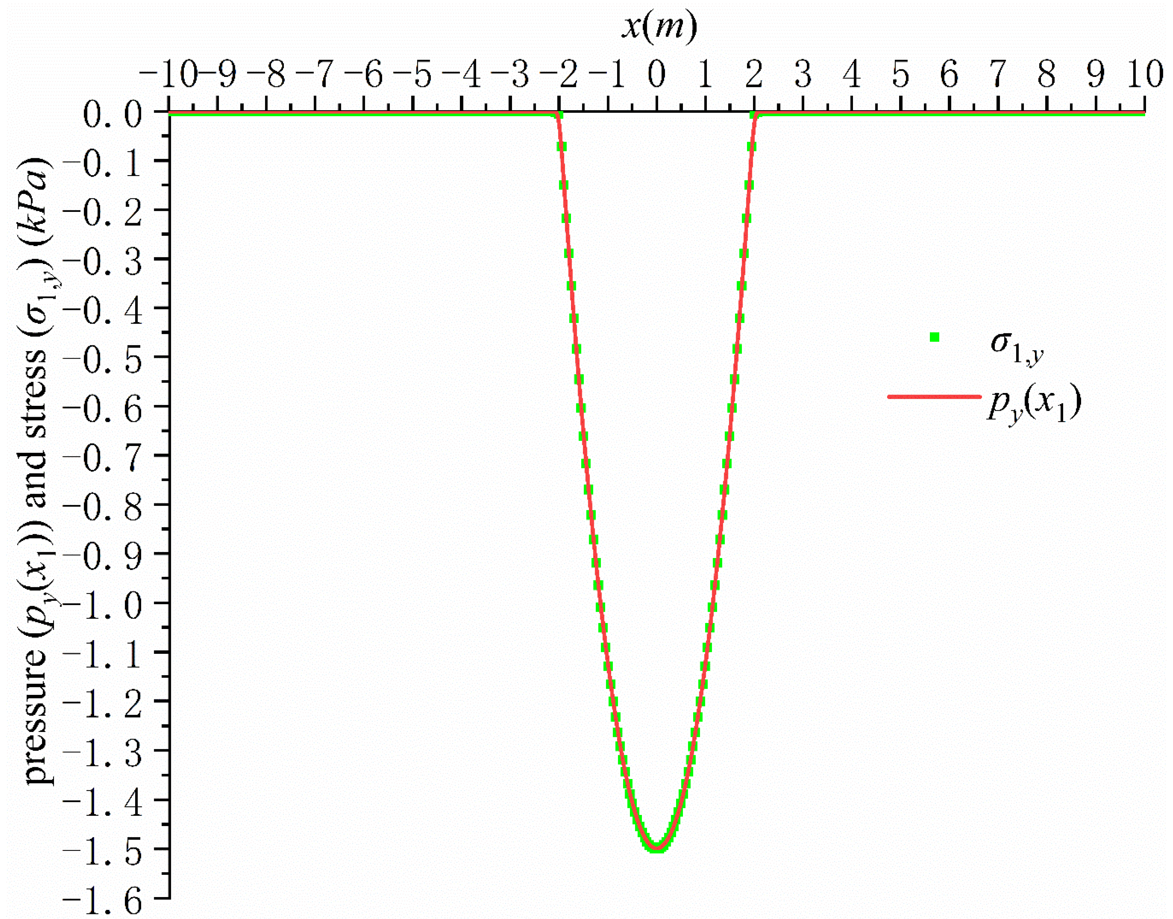
According to the given known conditions, the solution process in Section 3 can be used to calculate the ${\phi }_j\left({\zeta }_j\right)$ and ${\psi }_j\left({\zeta }_j\right)$ of each layer ($j=1, 2$), and then the stress components ${\sigma }_{1,y}$ and ${\tau }_{1,xy}$ of the surface can be obtained by Equation (42). If ${\sigma }_{1,y}=p_y\left(x_1\right)$,${\tau }_{1,xy}=p_x\left(x_1\right)=0$, the stress boundary condition is satisfied. It can be seen from the calculation that the value of ${\tau }_{1,xy}$ on the surface is very small, basically equal to zero, and ${\sigma }_{1,y}$ is also basically equal to $p_y\left(x_1\right)$. Figure 2 shows the distribution curve of ${\sigma }_{1,y}$ and $p_y\left(x_1\right)$ at the surface. It can be seen that the vertical stress curve of the surface basically coincides with the load curve, which indicates that the stress boundary conditions on the surface are well satisfied.

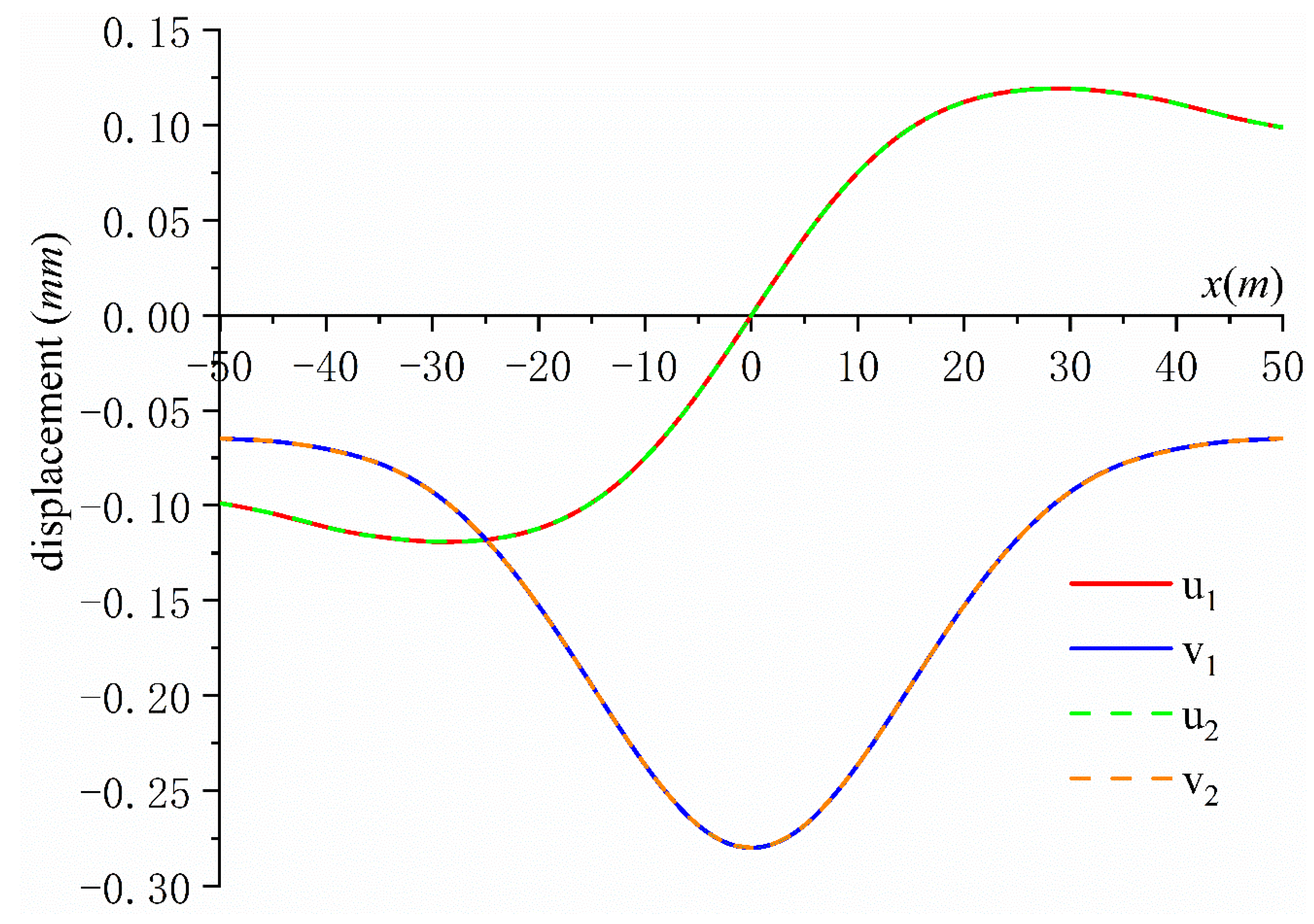
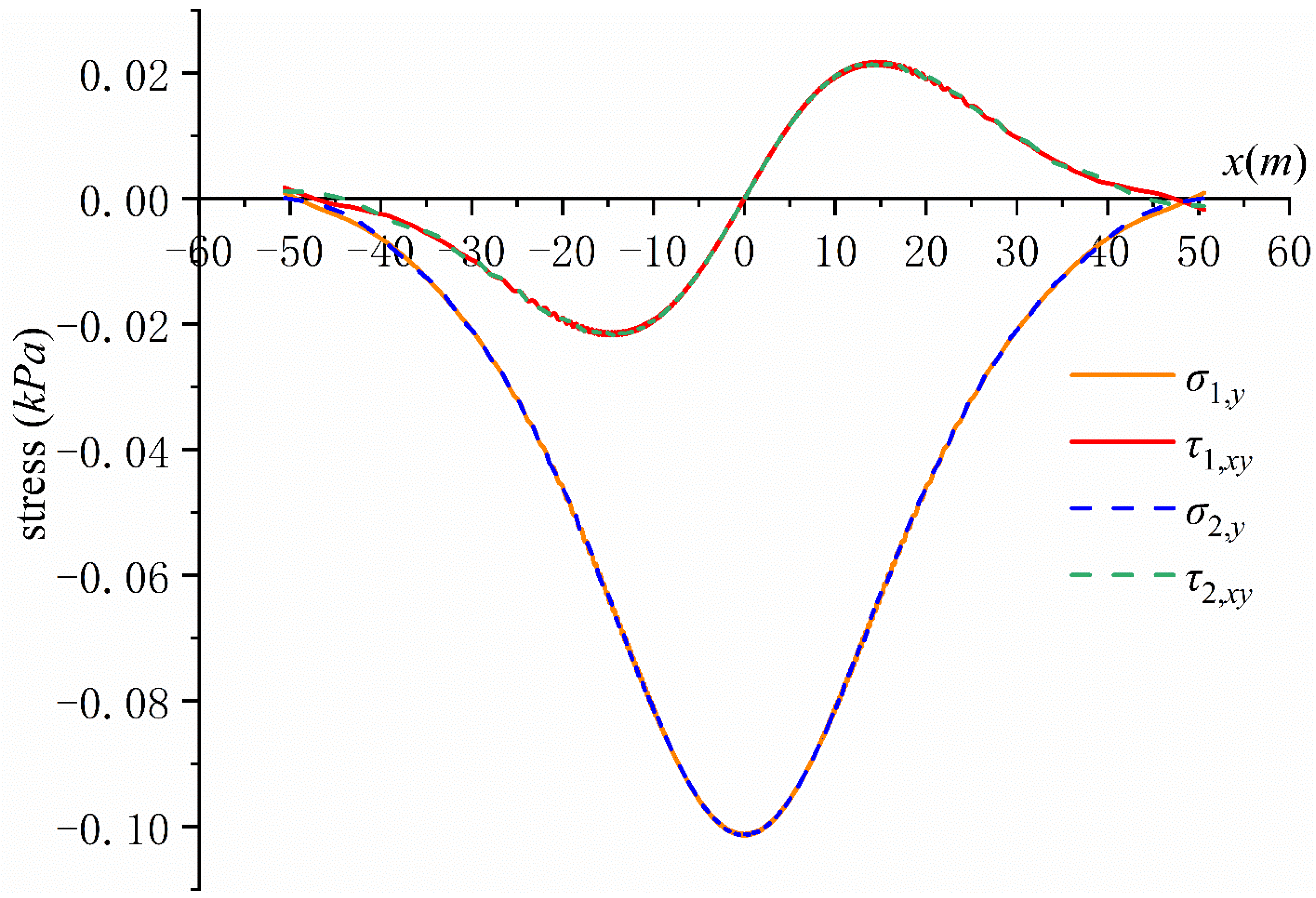
According to the calculated ${\phi }_j\left({\zeta }_j\right)$ and ${\psi }_j\left({\zeta }_j\right)$, the displacement and stress of each layer on the contact surface can also be obtained through Equations (41) and (42), therefore the continuity condition of the displacement and stress can be verified. Figure 3 shows the verification of the displacement continuity condition. It can be seen that $u_1\approx u_2$, $v_1\approx v_2$, where $u_1$ and $v_1$ are the x-direction displacement and y-direction displacement of the lower boundary of the first layer of soil, respectively, while $u_2$ and $v_2$ are the x-direction displacement and y-direction displacement of the same position of the upper boundary of the second layer of soil, respectively. Figure 4 shows the verification of the stress continuity condition, which shows that ${\sigma }_{1,y}\approx {\sigma }_{2,y}$, ${\tau }_{1,xy}\approx {\tau }_{2,xy}$. It can be seen from Figure 3 and Figure 4 that the displacement and stress continuity condition can also be satisfied very well. The maximum displacement in Figure 3 is $-0.255 \mathrm{mm}$, and compared with this, the maximum displacement of the lower boundary of the second layer is $1.3791294\times {10}^{-4} \mathrm{mm}$, which means the displacement boundary conditions of the lower boundary of the second layer are also very well satisfied.

4.2. Comparison with Numerical Method

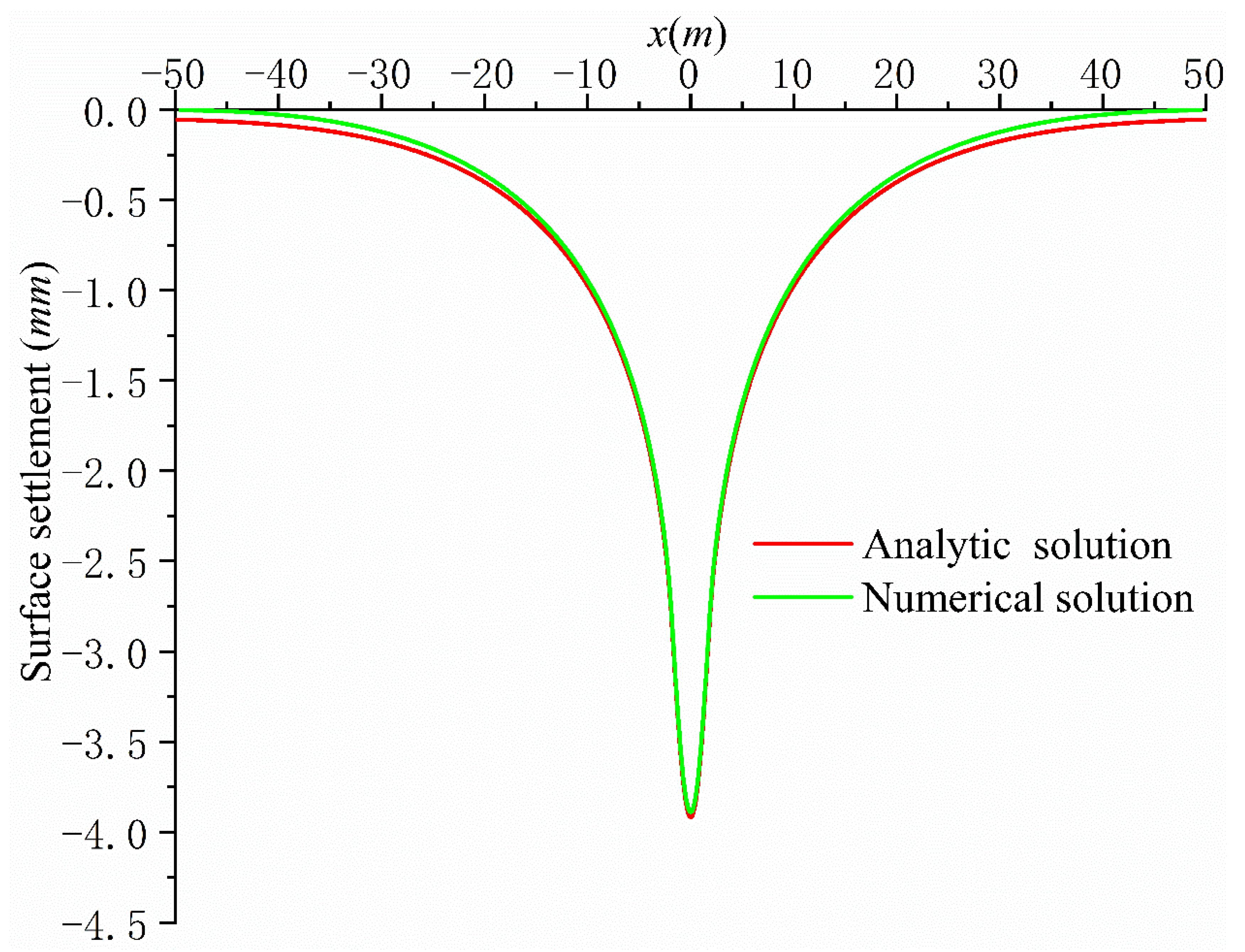
In Section 4.1, the surface stress boundary conditions, the displacement boundary condition of the lower boundary of the second layer and the stress and displacement continuity conditions between layers were verified. It was found that the boundary condition and the continuity conditions were very well satisfied; however, this is not enough to establish that the whole derivation process presented in this paper is correct. In order to verify the correctness of the whole derivation process, it is necessary to compare the calculation results of this paper with those of the numerical method. When the results of the two methods are in good agreement, the whole derivation process and the calculation program used in this paper are correct.

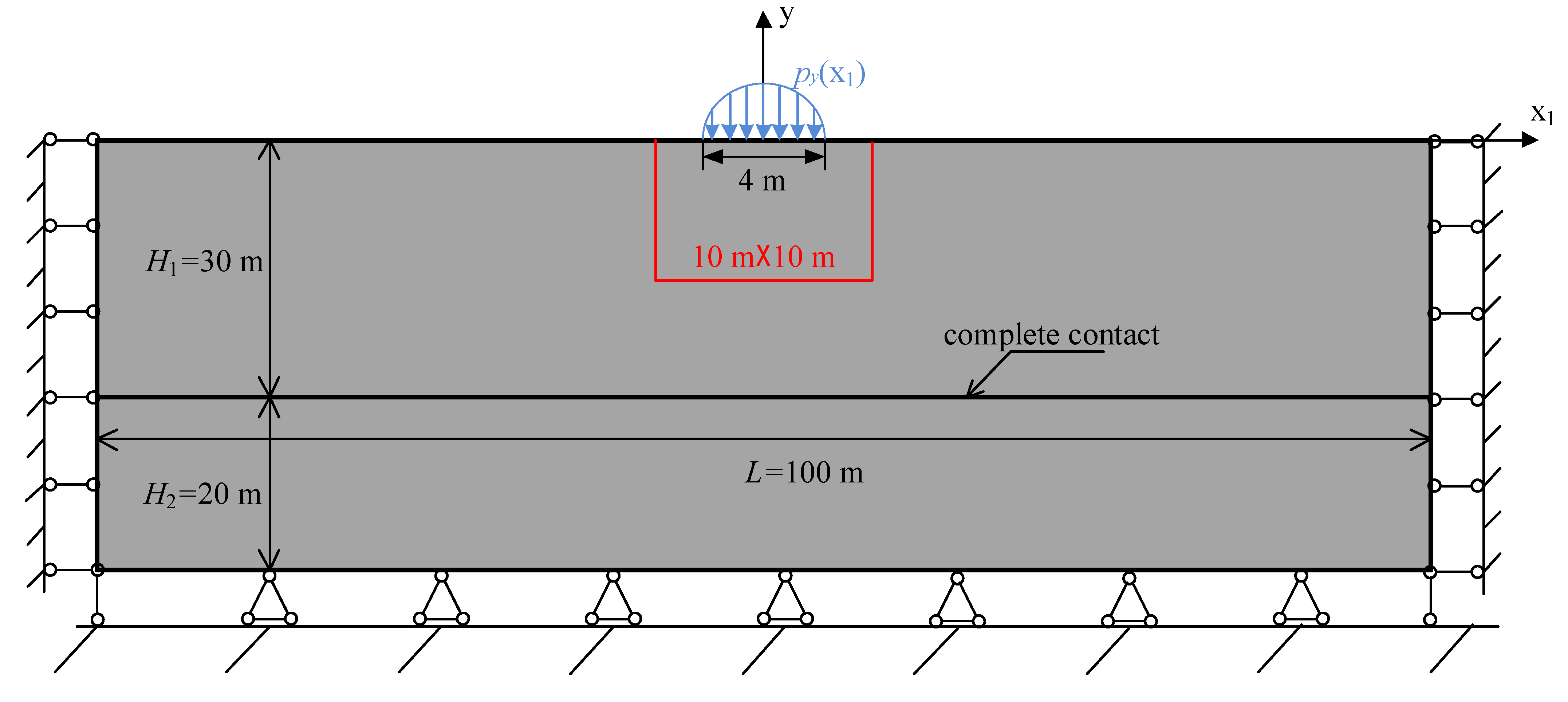
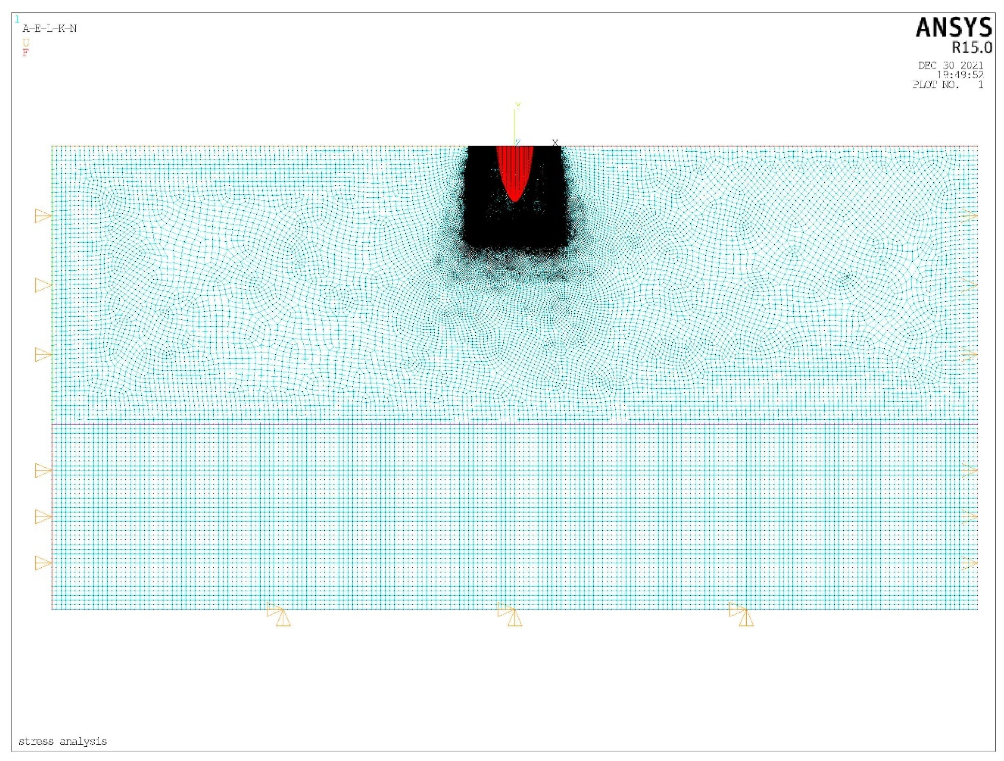
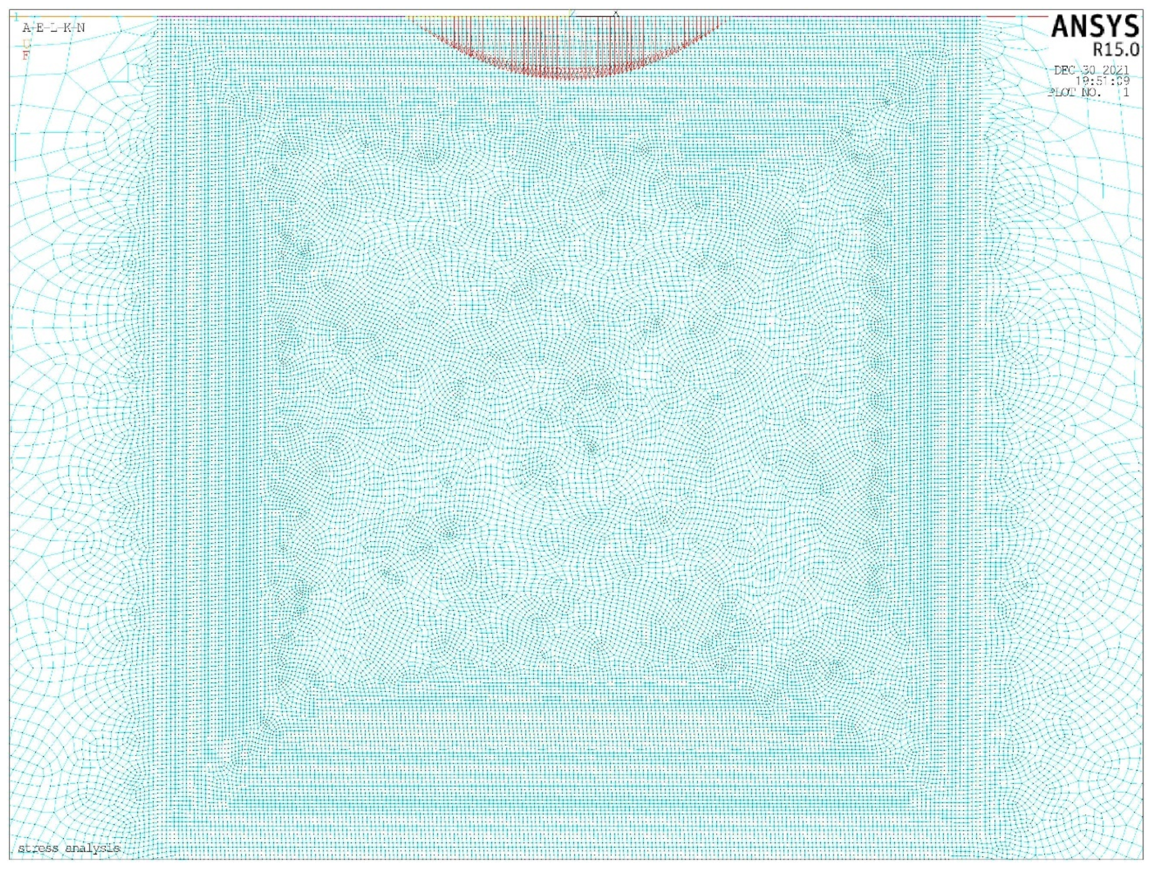
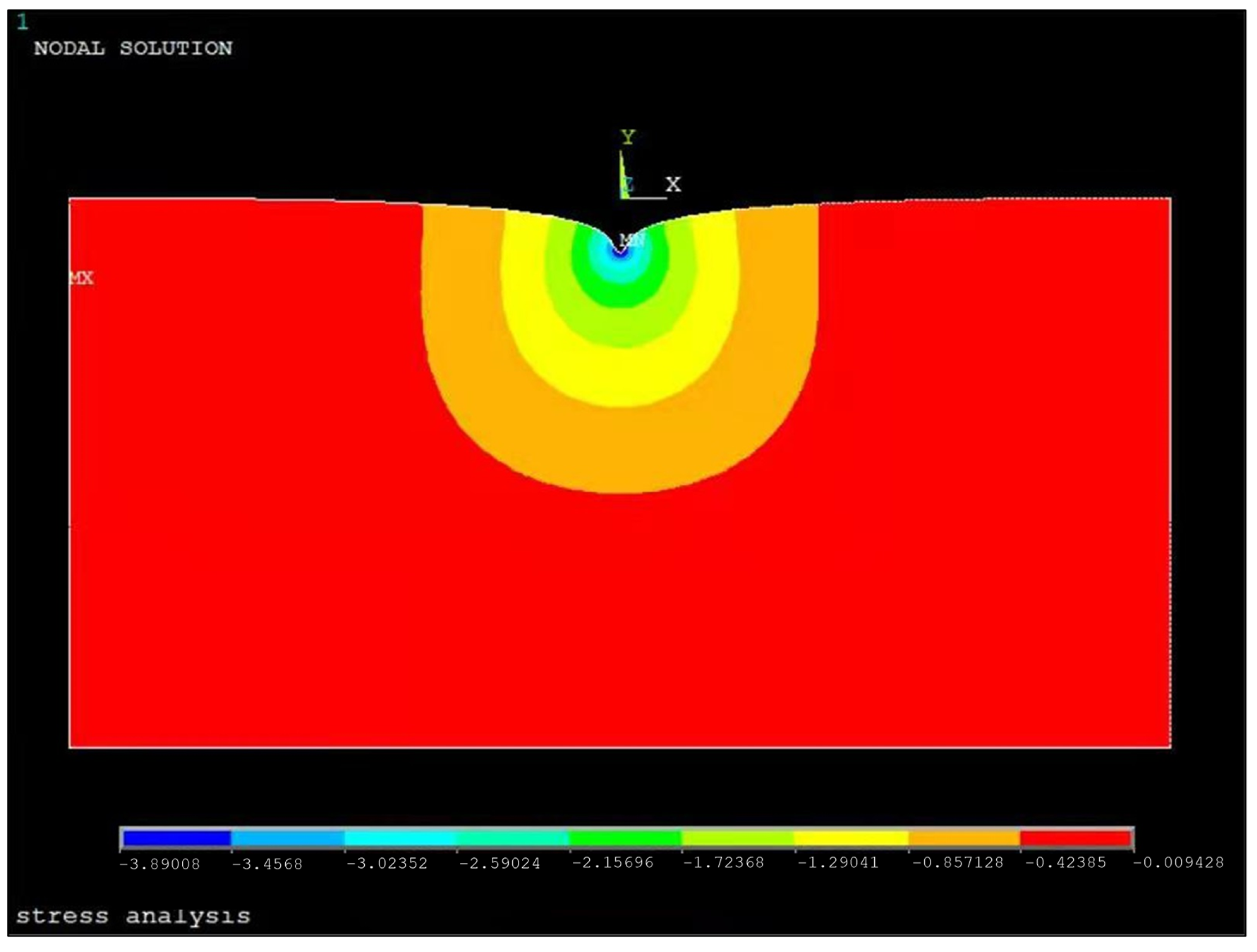
The schematic diagram of the ANSYS [30] model is shown in Figure 5. The model is divided into upper and lower soil layers. The width of the upper soil model is 100 m, the thickness is 30 m, the load action interval is $-2m\le x_1\le 2m,y=0$, the element type is plane42, the elastic modulus is $2.4 \mathrm{MPa}$, the Poisson’s ratio is 0.2, The element size in most areas is 0.5 (shown in Figure 6), and the element size is 0.05 in the area of $-2m\le x_1\le 2m,-10m\le y\le 0$ (shown in Figure 7),. The width of the lower soil model is 100 m, the thickness is 20 m, the element type is plane42, the elastic modulus is $5.2 \mathrm{MPa}$, the Poisson’s ratio is 0.3, and the element size is 0.5. The types of contact elements are targe169 (lower contact surface) and conta171 (upper contact surface). Horizontal displacement constraints are applied to the left and right sides of the model, and horizontal displacement constraints and vertical displacement constraints are applied to the bottom of the model. A parabolic distributed load is applied to the top of the model. The command flow is “f,i,fy,(nx(i)×nx(i)−4.0) ∗ 3/160”. There are 70,849 nodes and 70,684 elements in the model. Figure 8 shows the ANSYS deformation diagram. Figure 9 shows a comparison between the analytical solution and numerical solution of the surface settlement. ANSYS version 15.0 was used in this paper.

4.3. Influence of Base Pressure Distribution on Surface Settlement

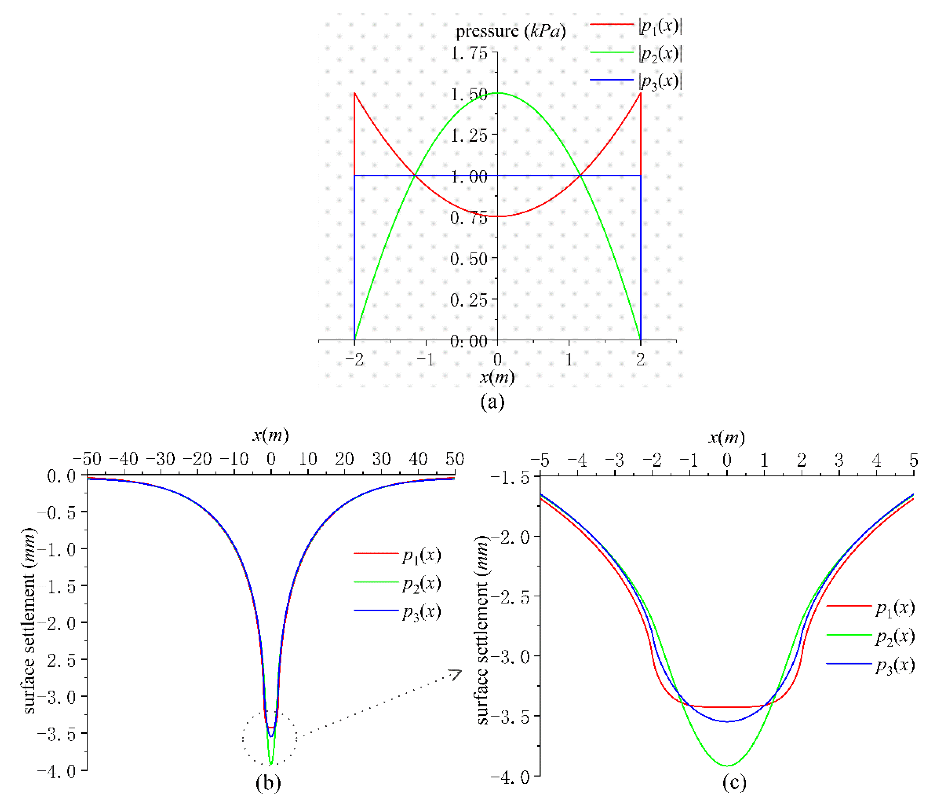
As shown in Figure 10a, three types of base pressure distribution under vertical action are discussed:

(1)

The concentration of base pressure is large at the edge: $p_{y1}\left(x_1\right)=\left(-3x_1^2-12\right)/16$;

(2)

The concentration of base pressure is large at the center: $p_{y2}\left(x_1\right)=-3\left(4-x_1^2\right)/8$;

(3)

Uniform distribution of base pressure: $p_{y3}\left(x_1\right)=-1$.

In order to compare the influence of load distribution on surface settlement, the resultant forces of the three types of base pressure distribution are the same, and they are all $4 \mathrm{kPa}$. The other parameters are the same as those described in Section 4.1, and the surface settlement that they caused are shown in Figure 10b,c.

It can be seen from Figure 10 that the surface settlement caused by the three types of base pressure distribution only shows certain differences near the foundation, and the maximum surface settlement occurs in the center of the foundation action area. When the load concentration at the center of the foundation is large, the surface settlement is the largest, followed by uniform distribution, and the surface settlement is smallest when the load concentration at the edge of the foundation is large. At the same time, it can be seen from Figure 10c that the surface settlement caused by the first distribution is approximately a horizontal line in the foundation action area. Only when the strip foundation is absolutely rigid and it is subjected to axial compression, can the bottom of the foundation sink evenly. Therefore, we can infer that the distribution form of the base pressure under the absolutely rigid strip foundation is close to this distribution form.

4.4. Influence of Layered Soil on Surface Settlement and Additional Stress Distribution in Soil

When $H_1=H_2=30 m$, $G_1=1.0 \mathrm{MPa}$, ${\mu }_1={\mu }_2=0.2$, the distribution of base pressure is $p_y\left(x_1\right)=-3\left(4-x_1^2\right)/8$, and other parameters are the same as those described in Section 4.1. Figure 11 shows the surface settlement curve when $G_2/G_1$ is $0.1$,$0.5$,$1.0$,$2.0$ and $10.0,$ respectively.

It can be seen from Figure 11 that the smaller the shear modulus ratio $G_2/G_1$, the greater the surface settlement. The influence of the change in $G_2/G_1$ on the surface settlement can be divided into two scenarios: when $G_2/G_1>1$, the change in $G_2/G_1$ has little influence on the surface settlement; when $G_2/G_1<1$, the change in $G_2/G_1$ has a great influence on the surface settlement.

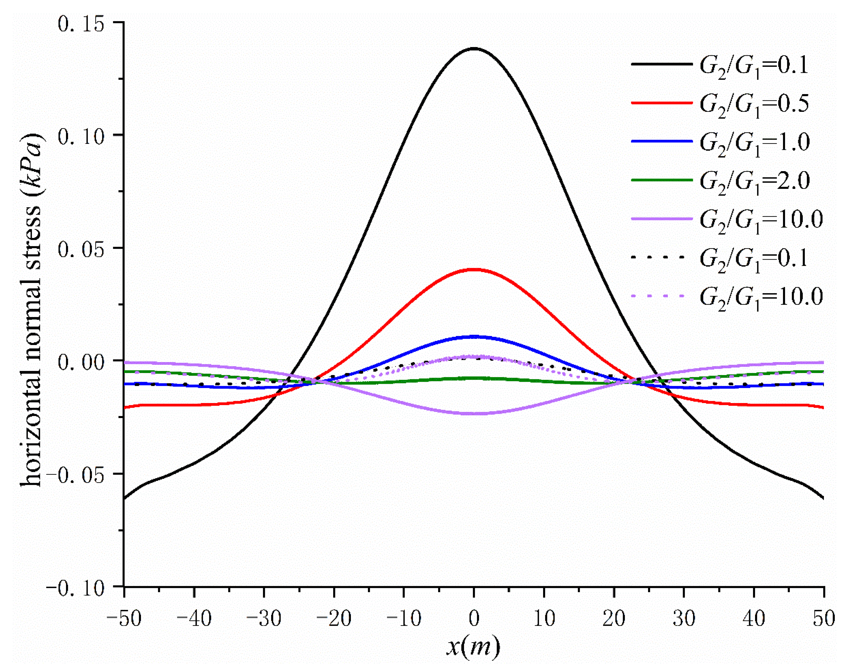
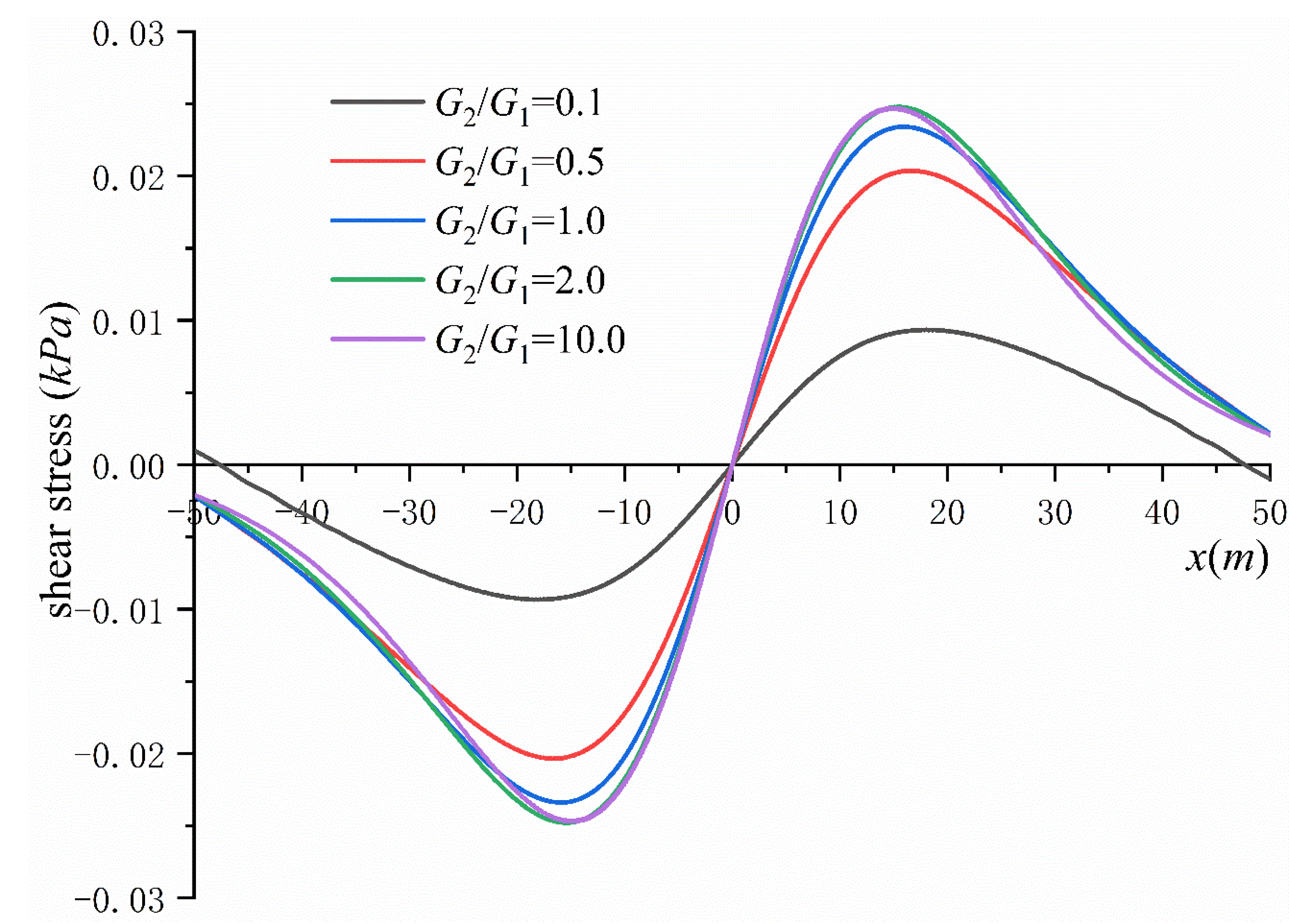
Figure 12 shows the ${\sigma }_{1,x}$ curves (solid line) of the lower boundary of the first layer when $G_2/G_1$ is 0.1, 0.5, 1.0, 2.0 and 10.0 and the ${\sigma }_{2,x}$ curves (dotted line) of the upper boundary of the second layer when $G_2/G_1$ is 0.1, and 10.0. Figure 13 shows the ${\sigma }_{1,y}$ curve on the contact surface, and Figure 14 shows the ${\tau }_{1,xy}$ curve on the contact surface.

It can be seen from Figure 12 that with the decrease in the shear modulus ratio $G_2/G_1$ of the two layers of soil, the maximum value of ${\sigma }_{1,x}$ (absolute value) of the lower boundary of the first layer of soil decreases at first and then increases, and the tensile stress occurs. Moreover, with the decrease in $G_2/G_1$, the tensile stress increases. Compared with the first layer, ${\sigma }_{2,x}$ on the upper boundary of the second layer is very small and the change in $G_2/G_1$ has little effect on ${\sigma }_{2,x}$. Therefore, this paper only shows the ${\sigma }_{2,x}$ curves when $G_2/G_1$ is 0.1, 10.0 respectively.

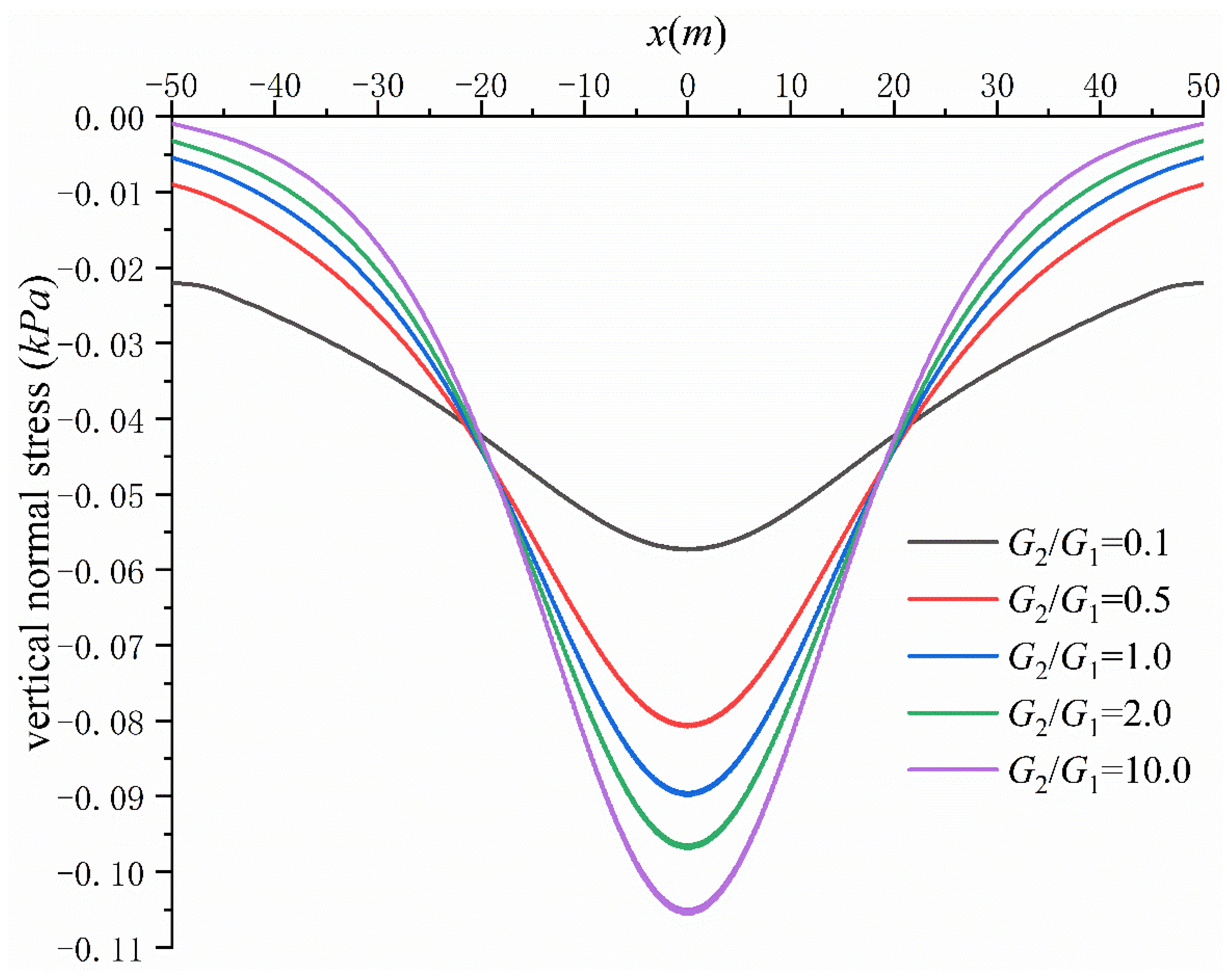
As can be seen from Figure 13, when the soft soil layer is covered by the hard soil layer ($G_2/G_1>1$), near $x=0$, the ${\sigma }_{1,y}$ (absolute value) on the contact surface is larger than that of homogeneous soil ($G_2/G_1=1$), but in the distance, it is smaller than that of homogeneous soil, that is, the stress concentration phenomenon occurs near $x=0$. When the hard soil layer covers the soft soil layer ($G_2/G_1<1$), the ${\sigma }_{1,y}$ on the contact surface is smaller near $x=0$ than that of the homogeneous soil layer, but larger in the distance than that of the homogeneous soil layer, which is known as the stress diffusion phenomenon. At this time, the vertical normal stress distribution on the contact surface is relatively uniform, so the vertical deformation of the lower soil will be relatively uniform, but it can be seen from Figure 12 that the horizontal tensile stress of the lower boundary of the upper soil will be relatively large.

It can be seen from Figure 14 that with the decrease in $G_2/G_1$, the shear stress ${\tau }_{1,xy}$ (absolute value) on the contact surface gradually decreases. When $G_2/G_1>1$, the change in $G_2/G_1$ has little effect on the shear stress distribution on the contact surface, while when $G_2/G_1<1$, the change in $G_2/G_1$ has a greater effect on the shear stress.

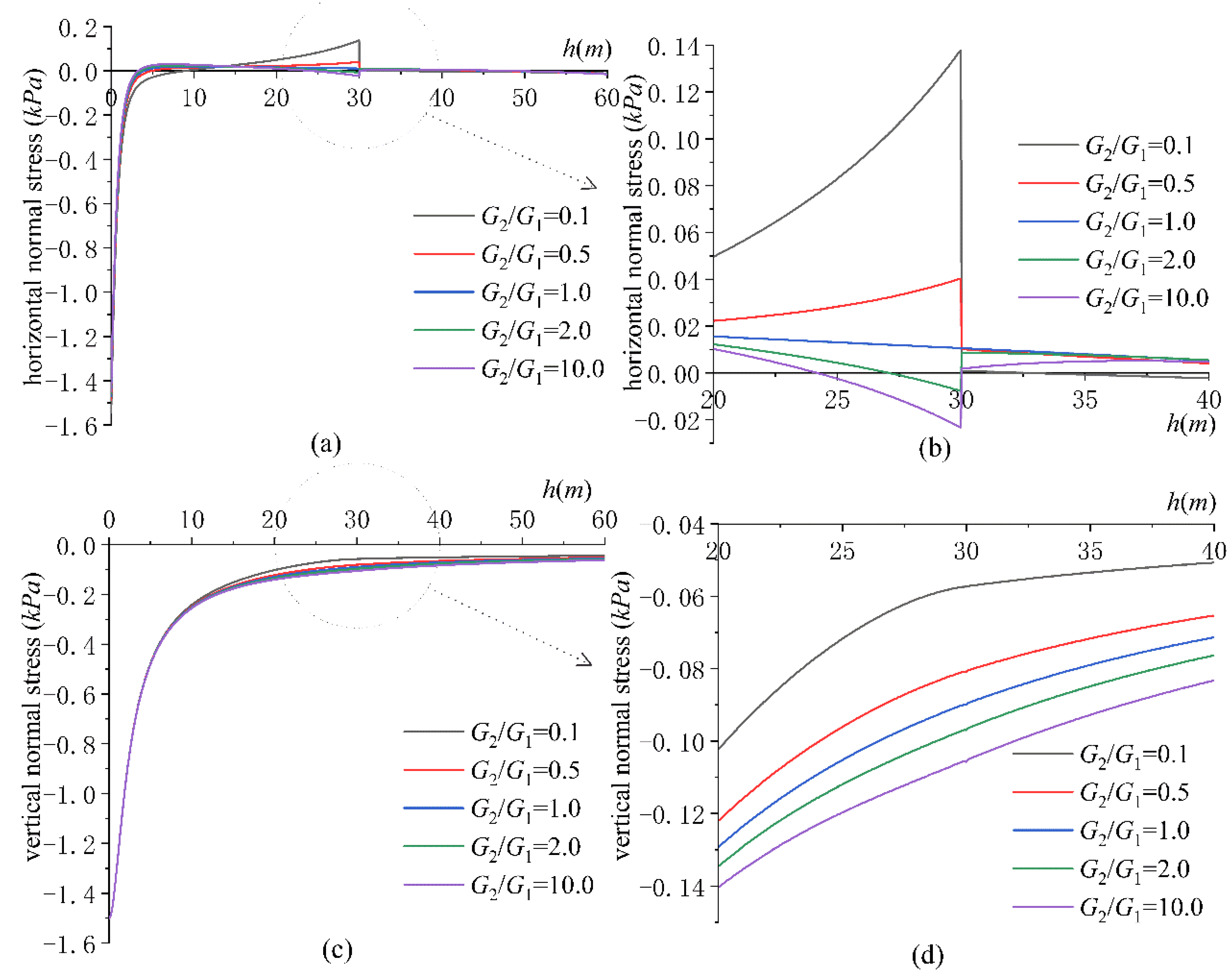
Taking the same parameters as described in Section 4.1, since the base pressure is symmetrical about the y-axis, there are only two normal stress components on the y-axis, and the shear stress component is $0$. Figure 15 shows the variation in the two normal stresses on the y-axis with depth $h$. At the surface, the horizontal normal stress is basically equal to the vertical normal stress. With the increase in $h$, the horizontal and vertical normal stress decay rapidly, and the decay speed of the horizontal normal stress is faster than that of the vertical normal stress. The horizontal normal stress at the surface is about $-1.5$, and it basically decays to zero at the depth of $h=4 m$. At the same time, it can be seen that due to the different material properties of the two layers of soil, the horizontal normal stress curve jumps at $h=30 m$ (contact surface).

5. Conclusions

The method proposed in this paper can be used to calculate the stress and displacement of multi-layer soil above bedrock under the action of a strip foundation. In fact, it is an analytical method, and the accuracy of its calculation results is related to the number of terms taken by the analytic function. Through the programming calculation, it was found that when the number of terms of the analytic function is 550, the accuracy of the calculation results is quite high, which can well meet the stress boundary condition, displacement boundary condition, and the stress and displacement continuity conditions. The results are in good agreement with those obtained by the finite element method.

In this paper, the effects of different distribution forms of base pressure and layered soil on the surface settlement and stress distribution inside the soil were analyzed by numerical examples. The results show that the surface settlement curves corresponding to the three types of basement pressure distribution are basically the same, but there are some differences near the foundation action area. When the distribution of the base pressure reaches the maximum in the center of the base, the displacement is at its maximum. The displacement caused by uniform distribution takes second place. When the base pressure is largest on both sides of the base, the displacement is the smallest. In the foundation action area, the surface settlement curve is approximately a horizontal straight line, which proves that the base pressure of a vertical sinking rigid foundation is similar to this distribution form.

For two-layer soil, the surface settlement decreases with the increase in the ratio of shear modulus ($G_2/G_1$), $G_1$ and $G_2$ are the shear modulus of the upper and lower soil, respectively. When the $G_2/G_1$ increases:

(1)

The maximum horizontal normal stress of the lower boundary of the upper soil first decreases and then increases, and when $G_2/G_1$ reaches a certain value, the tensile stress begins to appear;

(2)

The maximum vertical normal stress on the contact surface increases, while the vertical normal stress decreases at a distance from the foundation;

(3)

The shear stress on the contact surface only changes significantly when $G_2<G_1$.

References

Lu, A.; Zhang, N.; Liu, Y.; Sha, X. Analytic Solutions for Stress and Displacement of a Compressible Soil Layer above Bedrock. Int. J. Geomech.2021, 21, 04021232. [Google Scholar] [CrossRef]
Ghosh, P.; Sharma, A. Interference effect of two nearby strip footings on layered soil: Theory of elasticity approach. Acta Geotech.2010, 5, 189–198. [Google Scholar] [CrossRef]
Nova, R. Soil Mechanics; ISTE Ltd.: London, UK; John Wiley & Sons, Inc.: Hoboken, NJ, USA, 2010. [Google Scholar]
Song, F.; Wang, H.; Jiang, M. Analytically-based simplified formulas for circular tunnels with two liners in viscoelastic rock under anisotropic initial stresses. Constr. Build. Mater.2018, 175, 746–767. [Google Scholar] [CrossRef]
Carranza-Torres, C.; Fairhurst, C. The elasto-plastic response of underground excavations in rock masses that satisfy the Hoek–Brown failure criterion. Int. J. Rock Mech. Min. Sci.1999, 36, 777–809. [Google Scholar] [CrossRef]
Burmister, D.M. The General Theory of Stresses and Displacements in Layered Systems. I. J. Appl. Phys.1945, 16, 89–94. [Google Scholar] [CrossRef]
Burmister, D.M. The General Theory of Stresses and Displacements in Layered Soil Systems. II. J. Appl. Phys.1945, 16, 126–127. [Google Scholar] [CrossRef]
Burmister, D.M. The General Theory of Stresses and Displacements in Layered Soil Systems. III. J. Appl. Phys.1945, 16, 296–302. [Google Scholar] [CrossRef]
Barovich, D.; Kingsley, S.; Ku, T. Stresses on a thin strip or slab with different elastic properties from that of the substrate due to elliptically distributed load. Int. J. Eng. Sci.1964, 2, 253–268. [Google Scholar] [CrossRef]
Chen, W.T. Computation of stresses and displacements in a layered elastic medium. Int. J. Eng. Sci.1971, 9, 775–800. [Google Scholar] [CrossRef]
King, R.B. Elastic analysis of some punch problems for a layered medium. Int. J. Solids Struct.1987, 23, 1657–1664. [Google Scholar] [CrossRef]
Lee, J.; Jiang, L. Axisymmetric analysis of multi-layered transversely isotropic elastic media with general interlayer and support conditions. Struct. Eng. Mech.1994, 2, 49–62. [Google Scholar] [CrossRef]
Wang, J.; Fang, S. The state vector methods of axisymmetric problems for multilayered anisotropic elastic system. Mech. Res. Commun.1999, 26, 673–678. [Google Scholar] [CrossRef]
Wang, W.; Ishikawa, H. A method for linear elasto-static analysis of multi-layered axisymmetrical bodies using Hankel’s transform. Comput. Mech.2001, 27, 474–483. [Google Scholar] [CrossRef]
Polonsky, I.A.; Keer, L.M. Stress Analysis of Layered Elastic Solids with Cracks Using the Fast Fourier Transform and Conjugate Gradient Techniques. J. Appl. Mech.2001, 68, 708–714. [Google Scholar] [CrossRef]
Zeng, S.; Liang, R. A fundamental solution of a multilayered half-space due to an impulsive ring source. Soil Dyn. Earthq. Eng.2002, 22, 541–550. [Google Scholar] [CrossRef]
Lu, J.-F.; Hanyga, A. Fundamental solution for a layered porous half space subject to a vertical point force or a point fluid source. Comput. Mech.2004, 35, 376–391. [Google Scholar] [CrossRef]
Yue, Z.Q.; Xiao, H.T.; Tham, L.G.; Lee, C.F.; Yin, J.H. Stresses and displacements of a transversely isotropic elastic halfspace due to rectangular loadings. Eng. Anal. Bound.2005, 29, 647–671. [Google Scholar] [CrossRef]
Frétigny, C.; Chateauminois, A. Solution for the elastic field in a layered medium under axisymmetric contact loading. J. Phys. D Appl. Phys.2007, 40, 5418–5426. [Google Scholar] [CrossRef]
Zhang, Z.; Li, Z. Analytical solutions for the layered geo-materials subjected to an arbitrary point load in the cartesian coordinate. Acta Mech. Solida Sin.2011, 24, 262–272. [Google Scholar] [CrossRef]
Kawana, F.; Horiuchi, S.; Terada, M.; Kubo, K.; Matsui, K. Theoretical Solution Based on Volumetric Strain of Elastic Multi Layered Structures under Axisymmetrically Distributed Load. In Proceedings of the 2013 Airfield & Highway Pavement Conference: Sustainable and Efficient Pavements, Los Angeles, CA, USA, 9–12 June 2013; pp. 383–394. [Google Scholar]
Vasu, T.S.; Bhandakkar, T.K. Semi-analytical solution to plane strain loading of elastic layered coating on an elastic substrate. Sadhana2015, 40, 2221–2238. [Google Scholar] [CrossRef] [Green Version]
Zhang, P.; Liu, J.; Lin, G.; Wang, W. Elastic displacement fields of multi-layered transversely isotropic materials under rectangular loads. Eur. J. Environ. Civ. Eng.2018, 22, 1060–1088. [Google Scholar] [CrossRef]
Tokovyy, Y.V. Solutions of Axisymmetric Problems of Elasticity and Thermoelasticity for an Inhomogeneous Space and a Half Space. J. Math. Sci.2019, 240, 86–97. [Google Scholar] [CrossRef]
Andersen, S.; Levenberg, E.; Andersen, M.B. Efficient reevaluation of surface displacements in a layered elastic half-space. Int. J. Pavement Eng.2018, 21, 408–415. [Google Scholar] [CrossRef]
Wallace, E.R.; Chaise, T.; Nelias, D. Three-dimensional rolling/sliding contact on a viscoelastic layered half-space. J. Mech. Phys. Solids2020, 143, 104067. [Google Scholar] [CrossRef]
Levenberg, E.; Skar, A. Analytic pavement modelling with a fragmented layer. Int. J. Pavement Eng.2020, 1–13. [Google Scholar] [CrossRef]
Muskhelishvili, N.I. Some Basic Problems of the Mathematical Theory of Elasticity; Springer: Dordrecht, The Netherlands, 1977. [Google Scholar] [CrossRef] [Green Version]
Stolarski, T.; Nakasone, Y.; Yoshimoto, S. Engineering Analysis with ANSYS Software, 2nd ed.; Butterworth-Heinemann: Oxford, UK, 2018. [Google Scholar]
Figure 1.
The multi-layer soil above the bedrock is mapped on to the inner domain of the unit circle in the image plane: (a) multi-layer soil subjected to strip load and (b) each layer is mapped to the inner domain of the unit circle in the image plane.
Figure 2.
Verification of stress boundary conditions.
Figure 3.
Verification of displacement continuity condition.
Figure 4.
Verification of stress continuity condition.
Figure 5.
Schematic diagram of ANSYS model.
Figure 6.
ANSYS model diagram.
Figure 7.
Distribution of elements near the load.
Figure 8.
The deformation diagram of ANSYS.
Figure 9.
Comparison between analytical solution and numerical solution of surface settlement.
Figure 10.
Three types of base pressure distribution and the surface settlement they caused: (a) distribution of base pressure, (b) surface settlement, and (c) surface settlement near foundation.
Figure 11.
Effect of layered soil on surface settlement.
Figure 12.
Effect of layered soil on horizontal normal stress at interface.
Figure 13.
Effect of layered soil on vertical normal stress at interface.
Figure 14.
Effect of layered soil on shear stress at interface.
Figure 15.
Distribution of horizontal normal stress and vertical normal stress along y-axis. (a) Horizontal normal stress, (b) Local diagram of horizontal normal stress, (c) Vertical normal stress and (d) Local diagram of vertical normal stress.
Publisher’s Note: MDPI stays neutral with regard to jurisdictional claims in published maps and institutional affiliations.
Sha, X.; Lu, A.; Cai, H.; Yin, C.