Prediction of the Deformation of Aluminum Alloy Drill Pipes in Thermal Assembly Based on a BP Neural Network

Abstract

The connection between the steel joint and aluminum alloy pipe is the weak part of the aluminum alloy drill pipe. Practically, the interference connection between the aluminum alloy rod and the steel joint is usually realized by thermal assembly. In this paper, the relationship between the cooling water flow rate, initial heating temperature and the thermal deformation of the steel joint in interference thermal assembly was studied and predicted. Firstly, the temperature data of each measuring point of the steel joint were obtained by a thermal assembly experiment. Based on the theory of thermoelasticity, the analytical solution of the thermal deformation of the steel joint was studied. The temperature function was fitted by the least square method, and the calculated value of radial thermal deformation of the section was finally obtained. Based on the BP neural network algorithm, the thermal deformation of steel joint section was predicted. Besides, a prediction model was established, which was about the relationship between cooling water flow rate, initial heating temperature and interference. The magnitude of interference fit of steel joint was predicted. The magnitude of the interference fit of the steel joint was predicted. A polynomial model, exponential model and Gaussian model were adopted to predict the sectional deformation so as to compare and analyze the predictive performance of a BP neural network, among which the polynomial model was used to predict the magnitude of the interference fit. Through a comparative analysis of the fitting residual (RE) and sum of squares of the error (SSE), it can be known that a BP neural network has good prediction accuracy. The predicted results showed that the error of the prediction model increases with the increase of the heating temperature in the prediction model of the steel node interference and related factors. When the cooling water velocity hit 0.038 m/s, the prediction accuracy was the highest. The prediction error increases with the increase or decrease of the velocity. Especially when the velocity increases, the trend of error increasing became more obvious. The analysis shows that this method has better prediction accuracy.

1. Introduction

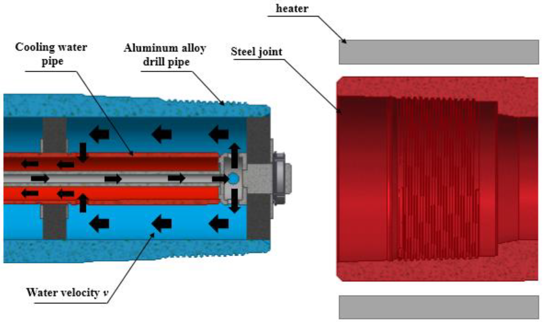
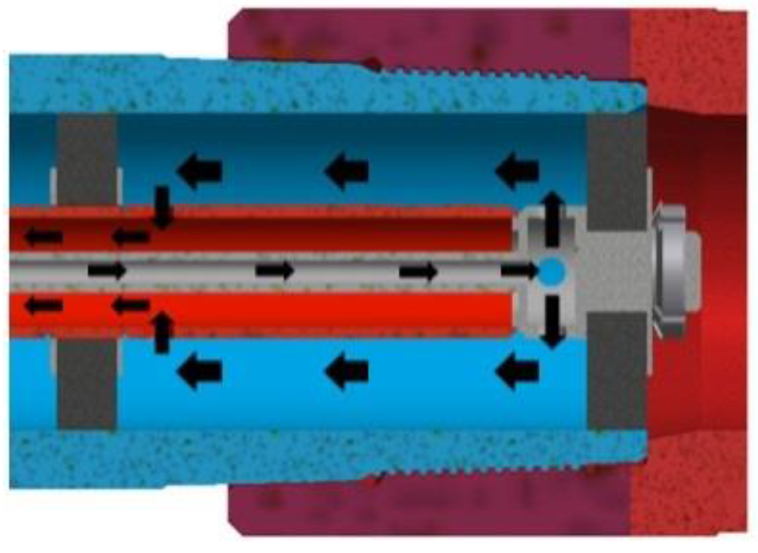
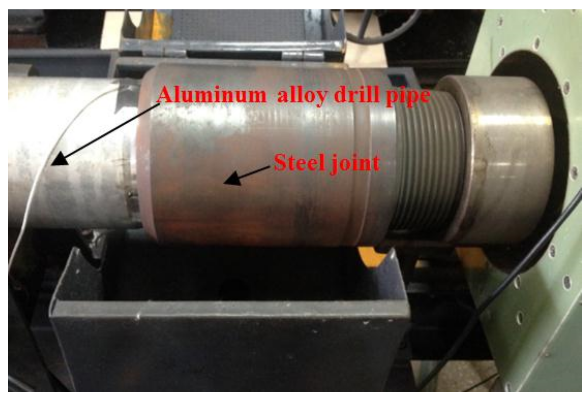
The steel drill pipe was widely used in traditional drillings. Owing to the high density of steel, the drilling depth was limited. With the increase of drilling depth, the weight of the steel drill pipe increased rapidly, resulting in a significant increase in the requirements for the capacity of drilling equipment. Therefore, for deep continental drilling and deep-water offshore drilling, it was very necessary to use light aluminum alloy drill pipe to improve drilling efficiency and reduce power consumption. Using an aluminum alloy drill pipe, more portable drilling equipment could be used at the same well depth, which greatly saved costs. For the aluminum alloy drill pipe, the connection between the steel joint and aluminum alloy pipe was not only the weak part, but also the main failure part of aluminum alloy drill pipes. Thus, the connection reliability would directly affect the reliability of the whole drill pipe.

Marcelo Igor [1] carried out a correlational study on the fatigue analysis of aluminum alloy drill pipe thermal assembly. The fatigue strength of the connection was improved by optimizing the thread. Sun, Y [2,3,4] used a finite element program and inverse heat conduction model to identify the heat transfer coefficient during thermal assembly in line with the experimental data and then obtained the correlation curve between cooling water flow and the convective heat transfer coefficient. Belkacem [5] studied the connection between ST 2024 aluminum alloy drill pipe and steel drill pipe in a curved hole trajectory. The research showed that the ST 2024 aluminum alloy drill pipe had a great influence on the critical load allowed for the combined load and stability loss of the drill string. ST 2024 aluminum alloy drill pipe had good wear resistance and corrosion resistance even at a high temperature.

In recent years, as the precision of machinery equipment and measurement technology develop, the precision level of modern precision engineering has entered the micro-nano era. The effects of thermal deformation on machinery mechanical precision cannot be ignored. Therefore, more and more attention has been paid to the study of the thermal expansion mechanism, accurate calculation and the measurement of thermal deformation by domestic and foreign industries.

It was of great significance to study the rule of metal thermal expansion for analyzing the mechanism of mechanical thermal deformation and for improving the practical application technology [6,7,8,9]. The thermal elasticity theory found numerous applications for solving thermal deformation problems of various new materials and complicated mechanical parts. Yaghoobi [10] studied n-order deformation theory based on the theory of thermodynamics. Hyae K. Y [11] studied the stress distribution of double-layer metal circular tube structures based on thermoelastic theory. In recent years, thermal deformation research methods have been introduced into high-end computer numerical control (CNC) machining equipment to research thermal errors [12,13,14]. Back propagation (BP) neural network is a kind of multilayer feedforward neural network trained by an error back propagation algorithm. It has become one of the most widely used neural network models. A BP neural network has a very strong nonlinear mapping capability; it could automatically sum up the functional relationship between input and output data through training without any prior formula, and thus it is widely used in modeling [15,16,17,18,19]. Ling [20] predicted the heat load based on a BP neural network–Markov prediction model. The results showed that compared with other heat load forecasting methods, the BP neural network had obvious advantages in predicting accurately, and this model resulted in a good heat load forecasting effect.

Zhu [21] introduced the BP neural network to establish a new effective thermal error model for machining centers. The validity of the method is validated by an experiment in a machining center. Qin [22,23] developed a method to model the thermal error of the spindle based on a selective integrated BP neural network. Each BP neural network model was given a weight, and the weights were optimized using a genetic algorithm. The prediction performance of the BP neural network model, multiple linear regression model and least squares support vector machine model were compared by machining center experiments. Zhou [24] proposed a BP neural network model to optimize the constitutive relationship of aluminum alloy. They predicted the strain rates of aluminum alloy materials under different conditions. By comparing the experimental data, it was found that the prediction accuracy of BP neural network model was good.

In this paper, the relationship between the cooling water flow rate, the initial heating temperature and the thermal deformation of steel joint in interference thermal assembly were studied and predicted. In the first section, through the thermal assembly experiment, the temperature data of the measuring points in the steel joint were obtained. In the second section, based on the theory of thermoelasticity, the analysis of the thermal deformation of steel joint was studied. The least square method fitting temperature function was adopted, and the calculated value of radial thermal deformation in the section was finally obtained. In the third section, the thermal deformation in the section of steel joint was predicted based on the BP neural network algorithm. Furthermore, the prediction model of the relationship between the three was established. The introduction of the polynomial model, exponential model and Gaussian model based on the least square method were contributed to conduct comparative analysis of BP neural network’ predictive performance. Finally, the prediction accuracy of the model was compared and analyzed.

2. Experiments of Thermal Assembly

2.1. Experimental Apparatus

The drill pipes are often assembled or disassembled during the drilling. If aluminum alloy drill pipes are directly connected by threads instead of steel joints, they will be severely worn due to assembly and disassembly. Therefore, it is necessary to assemble steel joints, which bear the force and abrasion directly during disassembly. In order to prevent the mechanical properties of aluminum alloy from decreasing due to a high temperature in the hot assembly, circulating cooling water is used to cool the interior of the aluminum alloy rod during the whole assembly.

The steel joint is inductively heated to the specified temperature; the aluminum alloy drill pipe is fixed, and the internal cooling water begins to circulate, as shown in Figure 1. The steel joint moves towards the drill pipe. When approaching the drill pipe, the steel joint starts to rotate, and the steel joint and aluminum alloy drill pipe begin to tighten until all the threads are screwed together. The assembly is completed as shown in Figure 2.

A temperature sensor is arranged at point B to collect the temperature as shown in Figure 3. The actual picture of the thermal assembly experiment is shown in Figure 4.

2.2. Experimental Results

Ensure constant thermal assembly velocity and that the ambient temperature is 22 °C. The minimum magnitude of interference fit required for this thermal assembly is 0.22 mm. When the thermal deformation of the steel joint is 0.22 mm, the corresponding initial heating temperature of the steel joint is about 300 °C. Therefore, the initial heating temperatures of steel joints are set at 300 °C, 400 °C and 500 °C, respectively. The initial temperature of internal cooling water is 20 °C, and the flow rates are set at 0.016 m/s, 0.038 m/s and 0.061 m/s, respectively. By the orthogonal experimental method, nine groups of experiments were carried out. The assembly is completed when all threads are screwed. Keeping a constant speed, 30 s are needed to complete assembly. After the assembly, the temperatures of point B are shown in

Table 1. Temperature of point B when the assembly is completed (°C).

v/m/s	T = 300 °C	T = 400 °C	T = 500 °C
0.016	290	379.6	474.5
0.038	286.1	370	443.1
0.061	282.6	364.5	401.3

and Figure 5.

As can be seen from Table 1, the nine data points represent the temperature measured at point B when the assembly is completed. The temperature of 300 °C, 400 °C and 500 °C represents three different initial heating temperatures of the steel joint, and 0.16, 0.038 and 0.061 represent three different cooling water flow rates.

As can be seen from Figure 5, there is little temperature difference in point B when the initial heating temperatures are low. However, as the initial heating temperatures increase, the cooling effect of increasing the cooling water flow rate of point B becomes more obvious.

3. Thermal Deformation Model for Steel Joint

We studied the thermal deformation of the steel joint during thermal assembly. This section is based on the relevant theories of thermoelasticity, separating the object of study into the multi-loop structures and working out the expressions of the relationship between temperature field function and stress, strain and displacement on the basis of specific equations so as to solve the problems concerned. Especially in the past, the thermal expansion of steel joints was considered to be a linear uniform expansion, but in fact it was not a linear expansion. Based on thermoelastic theory, the analytical formula of thermal expansion deformation in the same section is derived.

3.1. Study on Analytical Method of Steel Joint’s Thermal Deformation

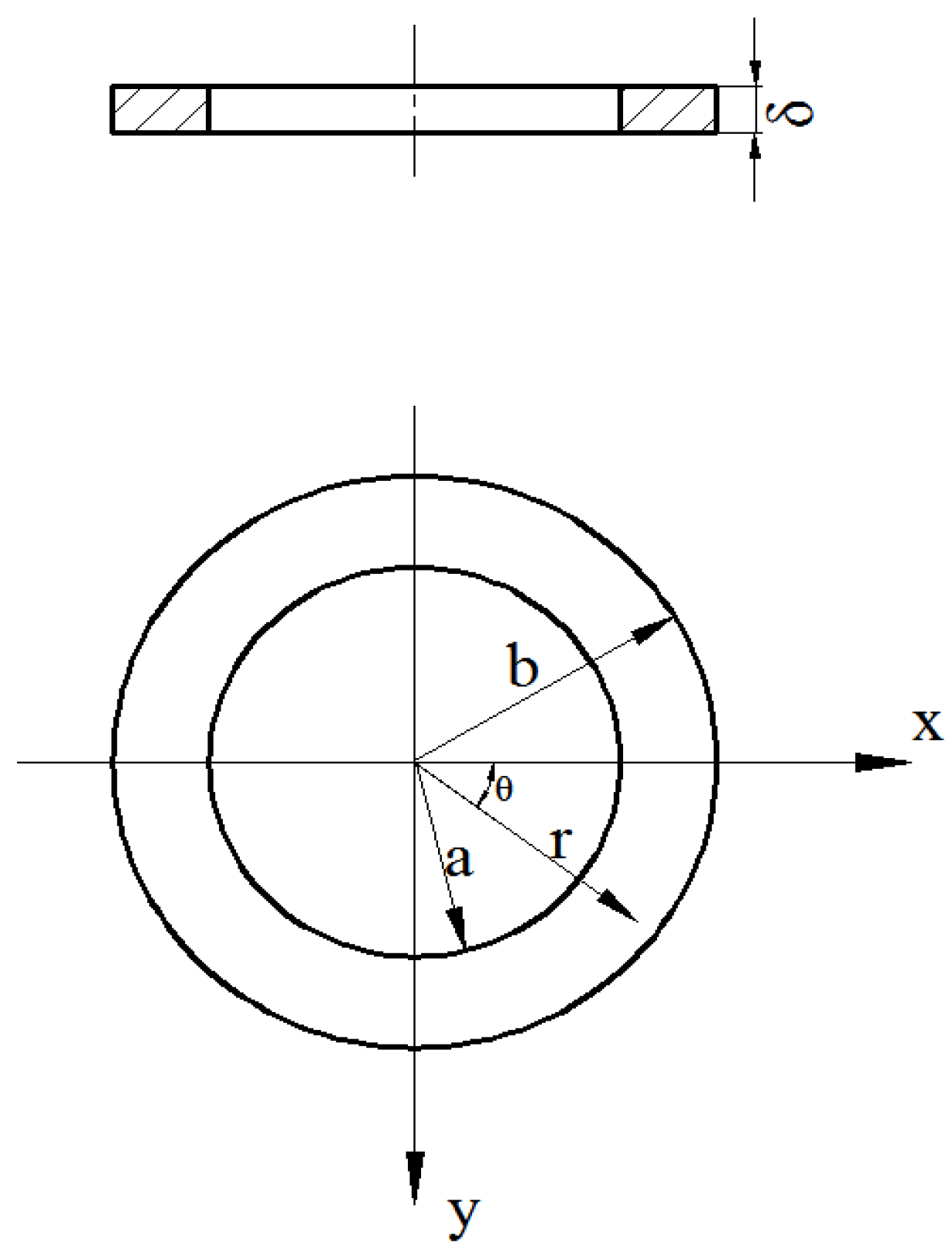
The joint is discretized into multiple thin rings, and the thickness of each ring is $\delta$. Thus, the thermal deformation of the joint becomes a plane stress problem, so ${\sigma }_z=0$, $\hspace{0.33em}{u}_r$ is the radial displacement, and r is the radius.

As shown in Figure 6, polar coordinates are adopted for the axisymmetric plane stress problem. The balance equation is as follows.

$$\left\{\begin{array}{l}\frac{\partial {\sigma }_r}{\partial r}+\frac{1}{r}\frac{\partial {\tau }_{r\theta }}{\partial \theta }+\frac{{\sigma }_r-{\sigma }_{\theta }}{r}=0\\ \frac{1}{r}\frac{\partial {\sigma }_{\theta }}{\partial \theta }+\frac{\partial {\tau }_{r\theta }}{\partial r}+\frac{2{\tau }_{r\theta }}{r}=0\end{array}\right.$$

(1)

where ${\sigma }_r$ is the normal stress of the radial; ${\sigma }_{\theta }$ is the normal stress of the radian and ${\tau }_{r\theta }$ is the shear stress.

The equilibrium equation is as follows:

$$\left\{\begin{array}{l}\frac{\partial {\sigma }_r}{\partial r}+\frac{{\sigma }_r-{\sigma }_{\theta }}{r}=0\\ \frac{\partial {\sigma }_{\theta }}{\partial \theta }=0\end{array}\right.$$

(2)

The geometric equation is:

$$\left\{\begin{array}{l}{\epsilon }_r=\frac{\partial u_r}{\partial r}\\ {\epsilon }_{\theta }=\frac{u_r}{r}\end{array}\right.$$

(3)

The physical equation is as follows:

$$\left\{\begin{array}{l}{\epsilon }_r=\frac{1}{E}({\sigma }_r-\mu {\sigma }_{\theta })+\alpha T\\ {\epsilon }_{\theta }=\frac{1}{E}({\sigma }_{\theta }-\mu {\sigma }_r)+\alpha T\end{array}\right.$$

(4)

wherein $\alpha$ is the linear expansion coefficient; $\mu$ is Poisson’s ratio and $E$ is the elastic modulus.

$$\left\{\begin{array}{l}{\sigma }_r=\frac{E}{1-{\mu }^2}({\epsilon }_r+\mu {\epsilon }_r)-\frac{E\alpha T}{1-\mu }\\ {\sigma }_{\theta }=\frac{E}{1-{\mu }^2}({\epsilon }_{\theta }+\mu {\epsilon }_r)-\frac{E\alpha T}{1-\mu }\end{array}\right.$$

(5)

Substituting Equation (3) into the formula above we have

$$\left\{\begin{array}{l}{\sigma }_r=\frac{E}{1-{\mu }^2}(\frac{d{u}_r}{dr}+\mu \frac{u_r}{r})-\frac{E\alpha T}{1-\mu }\\ {\sigma }_{\theta }=\frac{E}{1-{\mu }^2}(\frac{u_r}{r}+\mu \frac{d{u}_r}{dr})-\frac{E\alpha T}{1-\mu }\end{array}\right.$$

(6)

Making the subtraction for Formula (6) results in

$${\sigma }_r-{\sigma }_{\theta }=\frac{E}{1+\mu }({\epsilon }_r-{\epsilon }_{\theta })$$

(7)

Solving the derivative of r for the above equation and substituting the geometric Equation (3) into the above equation, we have

$${\sigma }_r-{\sigma }_{\theta }=\frac{E}{1+\mu }({\epsilon }_r-{\epsilon }_{\theta })=\frac{E}{1+\mu }(\frac{d{u}_r}{dr}-\frac{u_r}{r})$$

(8)

Solving the derivative of r for Equation (6) we obtain

$$\begin{array}{ll}\frac{\partial {\sigma }_r}{\partial r}& =\frac{E}{1-{\mu }^2}({\epsilon }_r^{\prime }+\mu {\epsilon }_{\theta }^{\prime })-\frac{E\alpha }{1-\mu }\cdot \frac{dT}{dr}\\ & =\frac{E}{1-{\mu }^2}\left[\frac{d}{dr}\left(\frac{d{u}_r}{dr}\right)+\mu \frac{d}{dr}\left(\frac{u_r}{r}\right)\right]-\frac{E\alpha }{1-\mu }\cdot \frac{dT}{dr}\\ & =\frac{E}{1-{\mu }^2}\left[\frac{d^2{u}_r}{d{r}^2}+\mu \left(\frac{u_r^{\prime }}{r}-\frac{u_r}{r^2}\right)\right]-\frac{E\alpha }{1-\mu }\cdot \frac{dT}{dr}\end{array}$$

(9)

If we substituted Formulas (8) and (9) into Formula (2), there would be

$$\frac{E}{1-{\mu }^2}\left[\frac{d^2{u}_r}{d{r}^2}+\mu \left(\frac{u_r^{\prime }}{r}-\frac{u_r}{r^2}\right)\right]-\frac{E\alpha }{1-\mu }\cdot \frac{dT}{dr}+\frac{E}{1+\mu }(\frac{d{u}_r}{r\cdot dr}-\frac{u_r}{r^2})=0$$

(10)

The above equation is thenmultiplied by $\left(1-{\mu }^2\right)/E$.

$$\begin{array}{ll}\alpha (1+\mu )\frac{dT}{dr}& =\frac{d^2{u}_r}{d{r}^2}+\frac{1}{r}\frac{d{u}_r}{dr}+\frac{1}{r^2}{u}_r\\ & =\frac{d^{}}{dr}\left[\frac{1}{r}\frac{d(r\cdot u_r)}{dr}\right]\end{array}$$

(11)

Integrating the equation, we have

$$\frac{d(r\cdot u_r)}{dr}\hspace{0.33em}=r\alpha (1+\mu )T+rC$$

(12)

Integrating the equation again, there would be

$$\hspace{0.33em}r\cdot u_r=\alpha (1+\mu ){\displaystyle {\int }_a^{r}T}rdr+C_1{r}^2+C_2$$

(13)

The displacement function is as follows:

$$\hspace{0.33em}{u}_r=\frac{\alpha (1+\mu )}{r}{\displaystyle {\int }_a^{r}T}rdr+C_{1}r+\frac{C_2}{r}$$

(14)

Getting the derivative of r for Formula (14), there would be

$$\hspace{0.33em}\frac{d{u}_r}{dr}=\alpha (1+\mu )\left(T-\frac{1}{r^2}{\displaystyle {\int }_a^{r}Trdr}\right)+C_1-\frac{C_2}{r^2}$$

(15)

With Formula (14) divided by $r$, there would be

$$\hspace{0.33em}\frac{u_r}{r}=\frac{\alpha (1+\mu )}{r^2}{\displaystyle {\int }_a^{r}T}rdr+C_1+\frac{C_2}{r^2}$$

(16)

Formulas (15) and (16) are then substituted into the ${\sigma }_r$ of Formula (5).

$$\begin{array}{ll}{\sigma }_r& =\frac{E}{1-{\mu }^2}\left[\alpha (1+\mu )\left(T-\frac{1}{r^2}{\displaystyle {\int }_a^{r}Trdr}\right)+C_1-\frac{C_2}{r^2}\right.\left. + \frac{\mu \alpha (1+\mu )}{r^2}{\displaystyle {\int }_a^{r}T}rdr+\mu C_1+\frac{\mu C_2}{r^2}\right]-\frac{E\alpha T}{1-\mu }\\ & =\frac{E}{1-{\mu }^2}\left[\alpha (1+\mu )T-\frac{\alpha (1-{\mu }^2)}{r^2}{\displaystyle {\int }_a^{r}T}rdr\right.\left.+(1+\mu )C_1-\frac{(1-\mu )C_2}{r^2}\right]-\frac{E\alpha T}{1-\mu }\\ & =-\frac{E\alpha }{r^2}{\displaystyle {\int }_a^{r}Trdr}+\frac{E{C}_1}{1-\mu }-\frac{E{C}_2}{r^2(1+\mu )}\end{array}$$

(17)

Owing to the boundary conditions ${\left.{\sigma }_r\right|}_{r=a}=0$ and ${\left.{\sigma }_r\right|}_{r=b}=0$, the equations containing integration constants $C_1$ and $C_2$ are:

$$\left\{\begin{array}{l}\frac{E{C}_1}{1-\mu }-\frac{E{C}_2}{a^2(1+\mu )}=0\\ -\frac{E\alpha }{r^2}{\displaystyle {\int }_a^{b}Trdr}+\frac{E{C}_1}{1-\mu }-\frac{E{C}_2}{b^2(1+\mu )}=0\end{array}\right.$$

(18)

We solve the above equations:

$$\left\{\begin{array}{l}{C}_1=\frac{\left(1-\mu \right)\alpha }{b^2-a^2}{\displaystyle {\int }_a^{b}Trdr}\\ C_2=(1+\mu )\frac{\alpha \cdot a^2}{b^2-a^2}{\displaystyle {\int }_a^{b}Trdr}\end{array}\right.$$

(19)

$C_1$ and $C_2$ are substituted into Formula (14), and the radius-directional thermal deformation function follows:

$$\hspace{0.33em}{u}_r=\frac{\alpha }{r}\left[(1+\mu ){\displaystyle {\int }_a^{r}T}rdr+\frac{\left(1-\mu \right)r^2+\left(1+\mu \right)a^2}{b^2-a^2}{\displaystyle {\int }_a^{b}Trdr}\right]$$

(20)

3.2. Establishing Temperature Function

The temperature T is a function of r. The function relationship between T and radius r is studied as follows.

Because the joints temperatures were changing uniformly, there is a linear relationship between the temperature function and r. The least square linear method is used to fit the temperature function T (r).

The linear equation is as follows:

$$T=c+d\cdot r+\epsilon$$

(21)

where $\epsilon$ is the deviation; and c, d are regression coefficients.

There would be

$${\displaystyle \sum _{i=1}^n{\epsilon }_i^2}={\displaystyle \sum _{i=1}^n{(T_i-c-d{r}_i)}^2}$$

(22)

The least-squares constraint would be:

$$Q_{}={\displaystyle \sum _{i=1}^n{\epsilon }_i^2}={\displaystyle \sum _{i=1}^n{(T_i-c-d{r}_i)}^2}=\min$$

(23)

where $Q_{}$ is the sum of the squared deviations.

We take partial derivatives of c and d, respectively, and set them equal to 0.

$$\left\{\begin{array}{l}\frac{\partial Q_{}}{\partial c}=2{\displaystyle \sum _{i=1}^n(T_i-c-d{r}_i)}=0\\ \frac{\partial Q_{}}{\partial d}=2{\displaystyle \sum _{i=1}^n(T_i-c-d{r}_i)}{r}_i=0\end{array}\right.$$

(24)

Further, there would be

$$\left\{\begin{array}{l}{\displaystyle \sum _{i=1}^n{T}_i-nc-d{\displaystyle \sum _{i=1}^n{r}_i}}=0\\ {\displaystyle \sum _{i=1}^n{T}_i{r}_i-c{\displaystyle \sum _{i=1}^n{r}_i}-d{\displaystyle \sum _{i=1}^n{r}_i^2}}=0\end{array}\right.$$

(25)

The estimated parameter values of c and d would be

$$\left\{\begin{array}{l}\widehat{d}=\frac{{\displaystyle \sum _{i=1}^n{r}_i T_i^{}}-n\overline{r} \overline{T}}{{\displaystyle \sum _{i=1}^n{r}_i^2}-n{\overline{r}}^2}\\ \widehat{c}= \overline{T}-\widehat{d} \overline{r}\end{array}\right.$$

(26)

where $\overline{T}$ is the average value of $T_i$, $\overline{T}=\frac{1}{n}{\displaystyle \sum _{i=1}^n{T}_i}$; and $\hspace{0.33em}\overline{r}$ is the average value of $r_i$, $\overline{r}=\frac{1}{n}{\displaystyle \sum _{i=1}^n{r}_i}$.

Because $a\le r_i\le b$, $r_1=a$ and $r_5=b$, $r_2$ to $r_4$ are equally spaced. For point B there are $r_1$ = 0.069, $r_2$ = 0.074, $r_3$ = 0.079, $r_4$ = 0.084 and $r_5$ = 0.089. According to Equation (26), we get the linear equation coefficients c and d of T in cross-sections of points B under 0.016 m/s, 0.038 m/s and 0.061 m/s at 300 °C, 400 °C, 500 °C, as shown in

Table 2. Linear equation coefficients of point B.

v/m/s	300 °C		400 °C		500 °C
	d	c	d	c	d	c
0.016	113.75	282.35	264.00	362.58	474.25	443.28
0.038	164.75	276.93	295.00	353.75	327.75	422.93
0.061	229.75	270.25	365.00	339.32	345.00	377.50

.

According to Formula (20), the sectional radial deformation is as shown in

Table 3. The sectional radial deformation of point B when all threads are screwed (mm).

v/m/s	T/°C	r/mm
		69	74	79	84	89
0.016	300	0.2229	0.2394	0.2744	0.3258	0.3922
	400	0.2992	0.3212	0.3681	0.4371	0.5262
	500	0.3797	0.4076	0.467	0.5546	0.6677
0.038	300	0.2218	0.2381	0.2729	0.3241	0.3901
	400	0.2939	0.3155	0.3615	0.4293	0.5169
	500	0.3533	0.3793	0.4347	0.5162	0.6214
0.061	300	0.2205	0.2367	0.2713	0.3221	0.3878
	400	0.2865	0.3076	0.3524	0.4185	0.5038
	500	0.3168	0.3401	0.3897	0.4628	0.5572

.

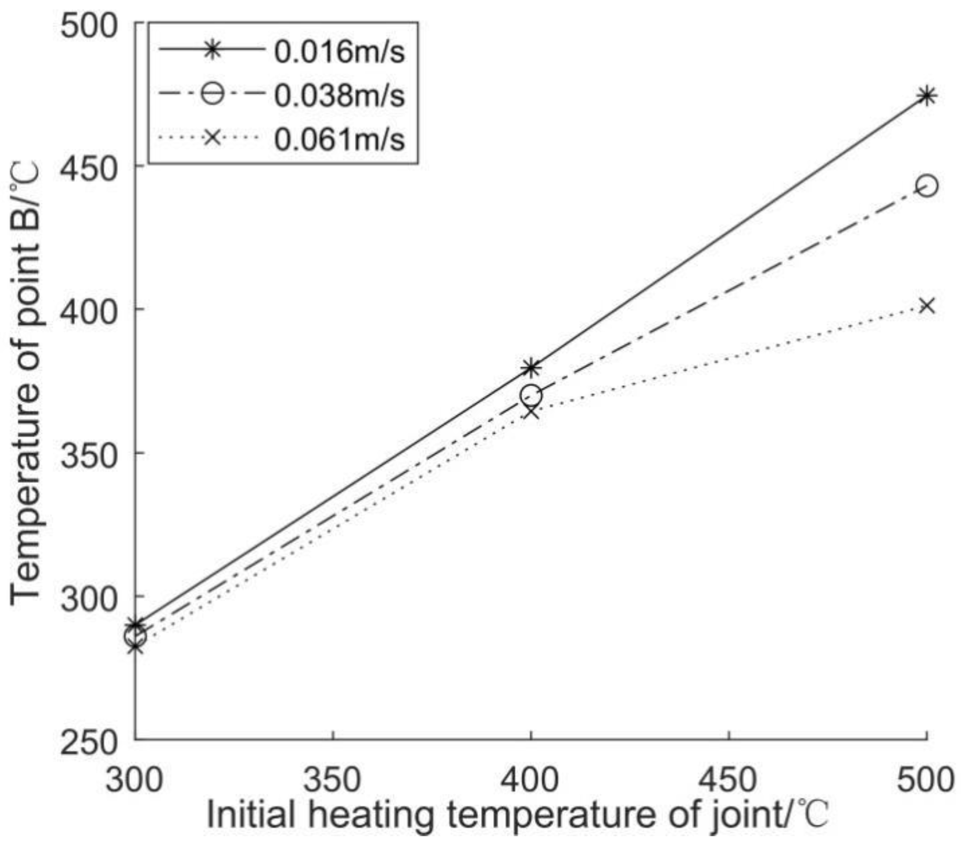
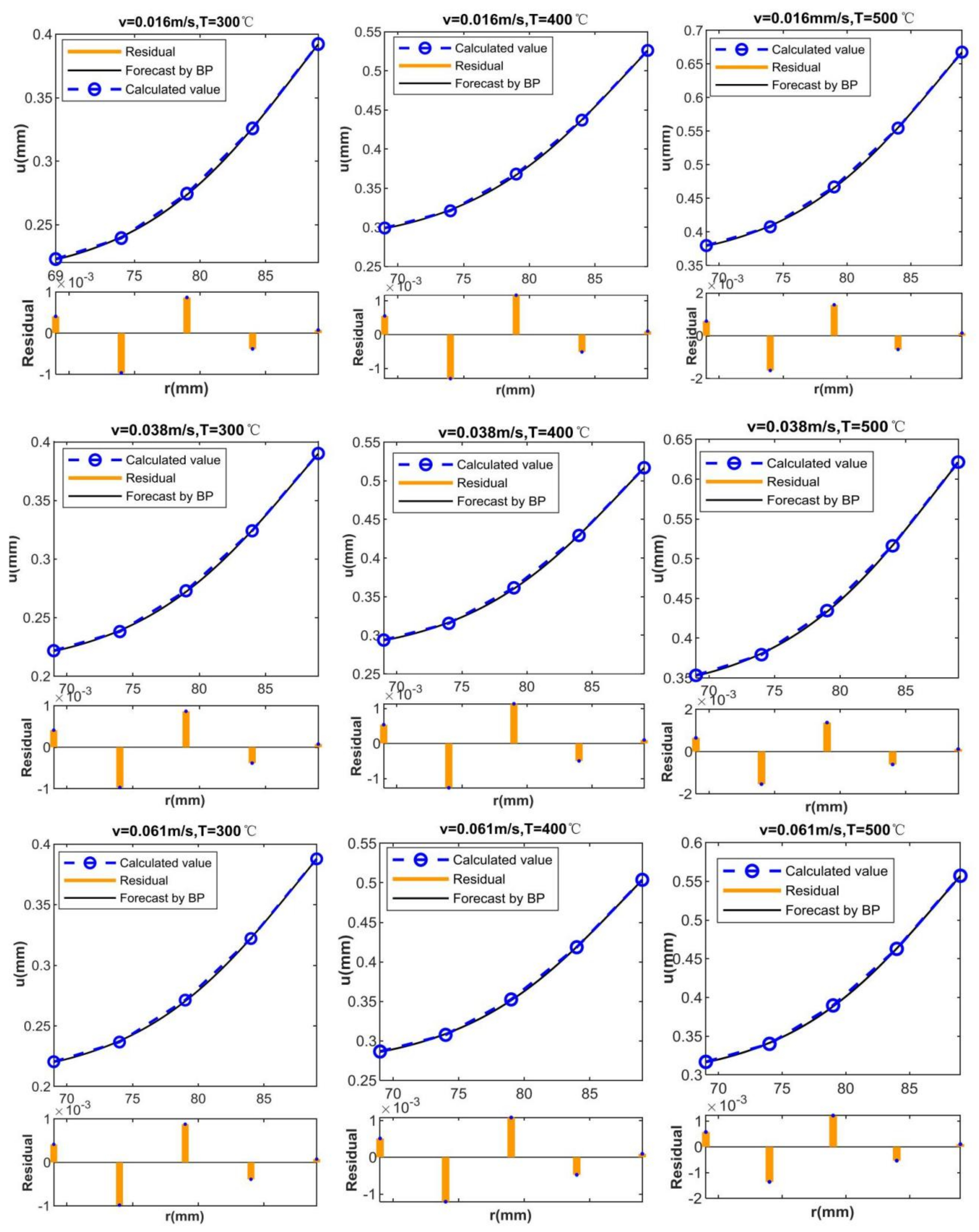
As can be seen from Figure 7, the increase rate of thermal deformation is increased with the increase of r. The deformations of the three cooling water flow rates are very similar when the temperature is 300 °C. With increasing initial heating temperatures, the deformation difference under three cooling water flow rates increases rapidly. In a word, with increasing initial heating temperatures, the change of the same cooling water flow has a greater influence on the thermal deformation.

4. BP Neural Network

In order to establish an accurate model of thermal deformation, a BP neural network algorithm was used in this paper to build the thermal deformation prediction model. A BP neural network algorithm is excellent at nonlinear mapping and self-learning, which is conducive to the realization of the multi-input single-output prediction model. By using this algorithm, the network can complete the correct mapping from the input space to the output space when the unknown sample data was added to the network during the thermal deformation prediction stage. The following mathematical model was established.

$$O_j^{}(t)=f\left(\left[{\displaystyle \sum _{\mathrm{i}=1}^{\mathrm{n}}{v}_{ij}}{x}_i^{}(t-{\tau }_{ij})\right]-L_j\right)$$

(27)

where $x_i$ is the input variable; $v_{ij}$ is the weight of the neuron from i to j; ${\tau }_{ij}$ is the synaptic delay between input and output; $L_j$ is the threshold of neuron j; $f(·)$ is neuronal activation function; and $O_j$ is the output error.

Because there are not many factors affecting thermal deformation, a BP neural network with single hidden layer is established in this paper; the topology is shown in Figure 8.

The fitting residual (RE), sum of squares of the error (SSE) and mean absolute error (MAE) are shown in Equations (28) to (30).

$$R{E}_i=x_i-{\widehat{x}}_i$$

(28)

$$SSE={\displaystyle \sum _{i=1}^N{(x_i-{\widehat{x}}_i)}^2}$$

(29)

$$MAE=\frac{1}{N}{\displaystyle \sum _{i=1}^N|x_i-{\widehat{x}}_i|}$$

(30)

5. Modeling and Analysis by BP Neural Network

5.1. Prediction of Sectional Radial Deformation

The topological structure of the BP neural network prediction model is 1-3-1. The input layer has one node receiving the data of radius r; the hidden layer has three nodes; the output layer has one node to output the radial thermal deformation of the section. The single hidden layer is selected. As the input layer and the hidden layer use the sigmoid function, the output layer uses the linear transfer function.

There are nine situations in total based on the statistics in Table 3. The training group has four training points and one control point in every situation. BP neural network prediction model is trained. The calculated thermal deformation predicted value and fitting residual are presented in Figure 9. Three precision models for predicting the radial deformation of sections are shown in

Table 4. The prediction model accuracy of sectional radial deformation.

v/m/s	T/°C	RE
		r = 69 mm	r = 74 mm	r = 79 mm	r = 84 mm	r = 89 mm
0.016	300	4.09E-04	−9.68E-04	8.68E-04	−3.84E-04	7.57E-05
	400	5.53E-04	−1.31E-03	1.17E-03	−5.16E-04	1.02E-04
	500	6.89E-04	−1.63E-03	1.45E-03	−6.41E-04	1.26E-04
0.038	300	4.11E-04	−9.70E-04	8.66E-04	−3.83E-04	7.57E-05
	400	5.36E-04	−1.27E-03	1.13E-03	−4.99E-04	9.87E-05
	500	6.52E-04	−1.54E-03	1.38E-03	−6.08E-04	1.20E-04
0.061	300	4.16E-04	−9.84E-04	8.80E-04	−3.89E-04	7.66E-05
	400	5.12E-04	−1.21E-03	1.08E-03	−4.77E-04	9.45E-05
	500	5.77E-04	−1.36E-03	1.22E-03	−5.37E-04	1.06E-04
SSE		2.60E-06	1.45E-05	1.16E-05	2.26E-06	8.80E-08
MAE		5.28E-04	1.25E-03	1.12E-03	4.93E-04	9.73E-05

.

As can be seen from Table 4, when r = 74 mm, the prediction error is the largest, and the prediction error decreases with the increase or decrease of radius r. When r increases to 89 mm, SSE is reduced to 8.8007E-08.

The polynomial model, exponential model and Gaussian model are, respectively, used for curve fitting, according to the principle of least squares. The fitting errors SSE and MAE of the three models are calculated and compared with the SSE and MAE of the BP neural network, which is shown in

Table 5. Comparison of prediction accuracy for different methods.

Error	Method	r = 69 mm	r = 74 mm	r = 79 mm	r = 84 mm	r = 89 mm
SSE	BP	2.60E-06	1.45E-05	1.16E-05	2.26E-06	8.80E-08
	Polynomial	2.43E-06	1.05E-05	1.14E-06	7.85E-06	3.66E-06
	Exponential	2.60E-03	3.86E-04	1.54E-03	3.73E-04	8.89E-04
	Gaussian	3.14E-03	2.86E-04	1.21E-03	2.78E-04	1.72E-03
MAE	BP	5.28E-04	1.25E-03	1.12E-03	4.93E-04	9.73E-05
	Polynomial	4.02E-04	1.03E-03	3.02E-04	8.15E-04	5.33E-04
	Exponential	1.67E-02	6.43E-03	1.28E-02	6.32E-03	9.76E-03
	Gaussian	1.82E-02	4.73E-03	1.08E-02	4.35E-03	1.29E-02

.

It can be seen that the SSE and MAE of the BP neural network are smaller than those of the exponential model and the Gaussian model in Table 5. Therefore, the BP neural network is significantly better than the exponential model and the Gaussian model in terms of prediction accuracy. According to Figure 10, the SSE and MAE of the BP neural network are larger than those of the polynomial model when r < 83 mm; therefore, it is concluded that the polynomial model is better than the BP neural network under this condition. Because the SSE and MAE of the BP neural network are smaller than those of the polynomial model when r > 83 mm, thus it is concluded that the BP neural network is better than the polynomial model under this condition.

5.2. Prediction Results and Analysis for Magnitude of Interference Fit and Relevant Factors

In fact, during the assembly the magnitude of interference fit between the steel joint and the aluminum alloy drill pipe is equal to the steel joints’ thermal deformation. Factors affecting the magnitude of interference fit are the cooling water flow velocity and the initial heating temperature of the steel joint. According to the discussion in Section 3, the relation between different cooling water flow velocities, initial heating temperatures and the magnitudes of interference fit are shown in the

Table 6. Thermal deformation of steel joint when all threads are screwed (mm).

v/m/s	T/°C
	300	400	500
0.016	0.2229	0.2992	0.3797
0.038	0.2218	0.2939	0.3533
0.061	0.2205	0.2865	0.3168

. The data of Table 6 are used as the BP neural network training group.

This BP neural network prediction model is a 2-7-1 topological structure. The input layer has two nodes for receiving the flow rate of cooling water and the initial heating temperature of the joint; the hidden layer has seven nodes, and the output layer has one node to the output thermal deformation of the steel joint; the hidden layer is individual. As the input layer and the hidden layer use the sigmoid function, the output layer uses the linear transfer function. After training, the prediction model of the relation between the interference of the steel joint, the flow rate of cooling water and the initial heating temperature of the steel joint is obtained, as shown in Figure 11.

As can be seen from in

Table 7. The prediction model accuracy of BP.

v/m/s	RE			SSE	MAE
	T = 300 °C	T = 400 °C	T = 500 °C
0.016	−1.53E-02	−1.78E-04	9.75E-03	3.30E-04	8.42E-03
0.038	−4.25E-03	8.60E-03	−4.00E-04	9.22E-05	4.42E-03
0.061	6.80E-03	1.55E-02	−2.04E-02	7.03E-04	1.42E-02
SSE	3.00E-04	3.13E-04	5.13E-04	-	-
MAE	8.80E-03	8.80E-03	1.02E-02	-	-

, in terms of heating temperature, through the analysis of SSE and MAE, it can be seen that the prediction model error increases with the increase of the heating temperature. In terms of the cooling water flow rate, $SS{E}_{0.061}>SS{E}_{0.016}>SS{E}_{0.038}$, $MA{E}_{0.061}>MA{E}_{0.016}>MA{E}_{0.038}$. Therefore, when the flow rate is 0.038 m/s, the prediction accuracy gets the highest, and the prediction error increases with the increase or decrease of the flow rate; especially when the flow rate increases, the trend of the error increase is more obvious.

For a comparative analysis, a polynomial model based on the least squares method is used in this paper for surface fitting. The fitting errors RE, SSE and MAE of the polynomial model are calculated separately as shown in

Table 8. The prediction model accuracy of the polynomial model.

v/m/s	RE			SSE	MAE
	T = 300 °C	T = 400 °C	T = 500 °C
0.016	3.96E-03	7.64E-02	1.56E-01	3.03E-02	7.89E-02
0.038	−8.36E-02	−5.66E-04	7.39E-02	1.25E-02	5.27E-02
0.061	−1.57E-01	−6.49E-02	−4.04E-03	2.88E-02	7.52E-02
SSE	3.15E-02	1.00E-02	3.00E-02
MAE	8.14E-02	4.73E-02	7.81E-02

. The RE, SSE and MAE of the polynomial model are compared with the prediction errors SSE and MAE of the BP neural network, as shown in

Table 9. Comparison of accuracy of prediction models at different water velocities.

v/m/s	BP		Polynomial
	SSE	MAE	SSE	MAE
0.016	3.30E-04	8.42E-03	3.03E-02	7.89E-02
0.038	9.22E-05	4.42E-03	1.25E-02	5.27E-02
0.061	7.03E-04	1.42E-02	2.88E-02	7.52E-02

and

Table 10. Comparison of accuracy of prediction models at different initial heating temperatures.

T	BP		Polynomial
	SSE	MAE	SSE	MAE
300 °C	3.00E-04	8.80E-03	3.15E-02	8.14E-02
400 °C	3.13E-04	8.80E-03	1.00E-02	4.73E-02
500 °C	5.13E-04	1.02E-02	3.00E-02	7.81E-02

. Based on the statistics in Table 9 and Table 10, it can be seen that the errors of the BP neural network are smaller than the errors of polynomial model for different flow velocities and different initial heating temperatures. Therefore, the performance of the BP neural network is better than the polynomial model.

To sum up, the BP neural network prediction model has a high prediction accuracy for all kinds of thermal errors. This method can be used to effectively establish the prediction model of the magnitude of interference fit for thermal assembly.

6. Conclusions

The connection between the steel joint and the aluminum alloy pipe is the weak part of the aluminum alloy drill pipe and the main site of its failure. In actual operation, the interference connection between aluminum alloy rod body and steel joint is usually realized by thermal assembly. In this paper, the relationship among cooling water flow rate, initial heating temperature of steel joint and thermal deformation of steel joint in interference thermal assembly was studied and predicted based on a BP neural network algorithm. The thermal deformation of the steel joint was predicted.

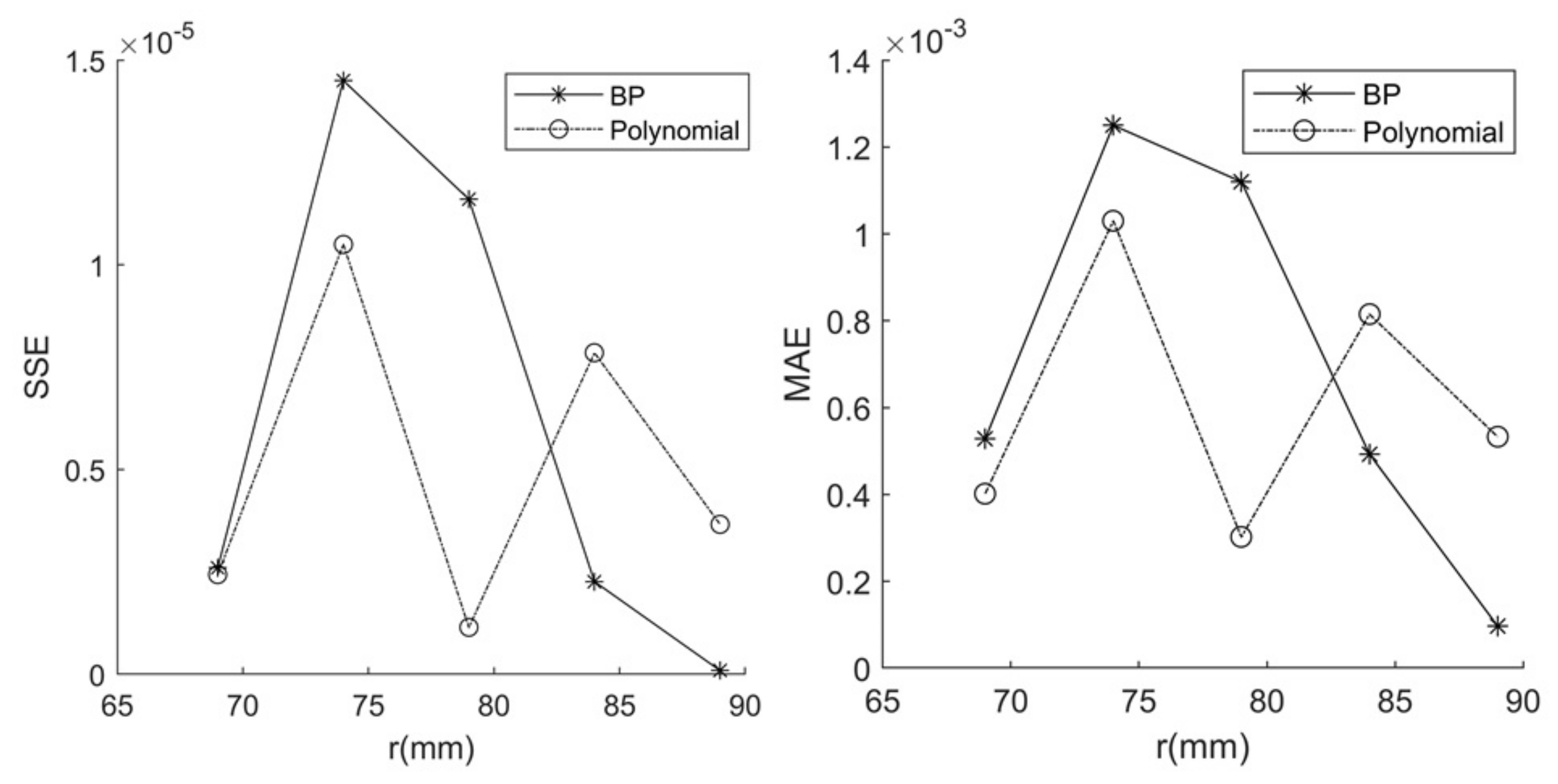
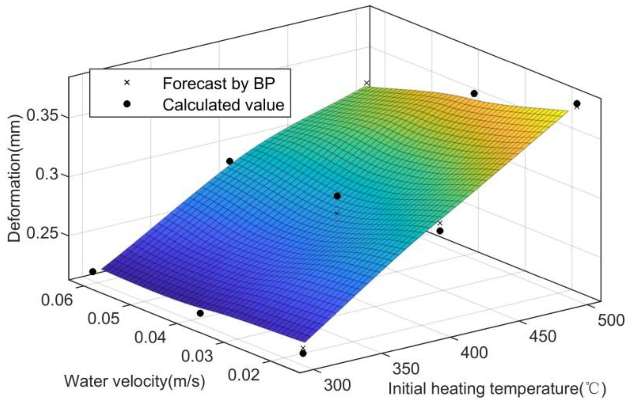
Furthermore, the magnitude of the interference fit of the steel joint was predicted as well, and the prediction results of the BP neural network were analyzed. A polynomial model, exponential model and Gaussian model based on the least square method were adopted to predict the sectional deformation in order to compare and analyze the prediction performance of the BP neural network. A polynomial model was used to predict the magnitude of the interference fit. Through a comparative analysis of SSE and MAE, it can be concluded that the BP neural network has good prediction accuracy.

Conclusions from the paper could be summarized as follows:

• The higher the initial heating temperature of steel joint, the greater the influence of the cooling water flow rate on the temperature and thermal deformation of steel joints.
• For the prediction model of thermal deformation in same section, when r = 74 mm, the prediction error was the largest. As the r increased or decreased, the prediction error decreased.
• For the prediction model of the magnitude of interference fit and relevant factors, with the increase of heating temperature, the prediction error increased. When the cooling water velocity was 0.038 m/s, the prediction accuracy was the highest. With the velocity increase or decrease, the prediction error increased. Especially when the velocity increased, the error’s trend to increase was more obvious.
• The polynomial model, exponential model and Gaussian model were, respectively, compared and analyzed with the BP neural network. By comparing the SSE and MAE of the prediction results of these methods, for the prediction of radial deformation of the section, the BP neural network is significantly better than the exponential model and Gaussian model. The BP neural network surpasses the polynomial model when r > 83 mm. The BP neural network outperforms the polynomial model when predicting the magnitude of interference fit and relevant factors.

A means of thermal deformation modeling for the thermal assembly of the aluminum alloy drill pipe is put forward, which can have better estimation accuracy and also provide theoretical guidance for the thermal assembly process of the aluminum alloy drill pipe. In the future, the BP neural network algorithm would be further improved to optimize the optimization performance, and the cold assembly of aluminum alloy drill pipe would be studied.